Sage Journals: Discover world-class research

Abstract

This article explores the use of fractional factorial designed experiments to help select the observations that are provided to a reinforcement learning agent for a hexapod robot trajectory-following task. A hexapod robot simulator is developed in the MATLAB Simscape environment and uses a central pattern generator consisting of 6 coupled Hopf oscillators and corresponding joint angle mapping functions to move the robot. The reinforcement learning agent is trained to control the hexapod using the deep deterministic policy gradient algorithm on a trajectory-following task. To test different combinations of seven potential observations, both quarter-fraction and eighth-fraction factorial designed experiments are proposed to reduce the number of runs from the maximum possible 128. Through the implementation of these designed experiments, regression models were formulated to predict which combinations of observations maximize the hexapod training reward. Model predictions were then validated using the simulator, and the corresponding trajectory-following capabilities of the hexapod were demonstrated. For the conditions used in this research, the observations that obtained the maximum final average reward are the hexapod's joint torques, body linear velocities, body orientation, body angular velocities, and body height above the ground.

Keywords

Reinforcement learning hexapod robot central pattern generator trajectory following observation selection fractional factorial designed experiment

Introduction

Mobile robotics play an increasingly important role to complete dangerous tasks in remote, hazardous, and extreme environments in the fields of surveillance, demining, inspection, rescue operations, and exploratory missions.¹ Such robots must be capable of overcoming difficult terrain in challenging environments without the need for human intervention. Walking hexapod robots are an ideal candidate for these roles as they offer several advantages over other mobile robotics platforms, including excellent maneuverability, versatility over complex terrain, better stability, redundancy to limb faults or failures, and adaptability to specific tasks or environments.² Research in the control of hexapod robots has progressed from traditional kinematics- and dynamics-based controllers, to biologically-inspired controllers using central pattern generators, optimization of gaits using genetic algorithms, and, more recently, machine learning using reinforcement learning (RL).¹

The current direction of the literature is for mobile robots to become increasingly independent of human operators using machine learning. Recent works have demonstrated the application of RL to train and control hexapod robots in complex environments for both path-planning navigation and complex locomotion tasks. RL allows a mobile robot to modify its behavior and walking gait in response to changes in terrain, external stimulus, and other inputs. RL agents are trained through a repetitive process where the hexapod must repeat a similar task many times to iteratively modify its behaviour to obtain a maximum reward for the given task. One such RL algorithm that is used in the present work is the deep deterministic policy gradient (DDPG).

There are numerous factors and parameters that influence the success of an RL agent. One of the most important factors is the selection of the observations which correspond to the measurements of the robot state and environment provided to the RL agent. In many machine-learning problems, the maximum amount of data available is provided to the learning algorithm; however, in practice, the observations needed to successfully learn a particular locomotion task will affect the physical hardware required and the design of the robot itself. There may be limitations in hardware cost, physical size constraints, or power requirements that necessitate the selection of a limited number of observations for a hexapod robot. The optimal combination of observations for a given RL task must be determined through testing; however, this process can lead to issues with constraints caused by the length of agent training time. Ibarz et al.³ discuss the importance of sample efficiency as many widely-used RL algorithms require millions of interactions over the course of training. Training can take a considerable amount of time, even within a simulation environment. This article presents the idea of using a fractional factorial designed experiment to gain insight into the relative importance of different observations using a reduced number of training runs so that engineering decisions can be made about the sensor package to include on a hexapod robot.

Originally developed for use in the fields of agriculture and industrial manufacturing, design of experiments (DOE) is a statistical methodology used to create experiments that are able to provide insight into the effects of various factors on a process result in the most efficient way possible.⁴ In the present research, the RL training routine is the “process,” the observations are treated as “process factors,” and the final average reward is taken as the measurable “process result.” With the overall goal of finding combinations of observations that maximize the final average reward, this research explores the potential application of a fractional factorial DOE in the selection of observations for a hexapod locomotion task.

RL in hexapod control

As noted by Coelho et al.,¹ the recent trend in controlling hexapod robots shows the emergence and increasing use of RL in the literature over the last half-dozen years. RL has significant advantages over other control methods in terms of reactions to external disturbances and changes to the environment.

A central pattern generator (CPG) can successfully produce smooth walking gaits for a hexapod, and further tuning and optimization of the gait can be performed using genetic algorithms. However, these methods are limited in that, once the gait has been determined, it typically remains fixed throughout deployment and cannot react to disturbances or environmental changes outside of those set in the predetermined gaits. RL agents, however, are able to react to external stimuli and, through varied and extensive training, have been shown to be able to generalize their behaviors to previously unseen circumstances. For example, Heess et al.⁵ demonstrated the emergence of complex locomotion behaviors for both a quadruped and a humanoid if provided sufficient observations during training in a complex and diverse simulation environment.

To demonstrate the variety of observations used for RL in the literature, the present authors carried out a systematic review, and the results are presented in Table 1. To narrow the scope of the literature search, this table only includes work which uses a hexapod or quadruped robot platform, as these robot configurations are similar in both performance and control requirements. Note that bipedal robots were excluded from this review as they are not statically stable and thus may require different observations.

Table 1.

Summary of observations used in the literature.

Reference	Joint angles	Joint angular velocities	Body orientation	Body angular velocities	Joint torques	Body displacements	Body linear velocities	Body height above ground	Ground contact	Previous actions	Others
Yang et al.⁶	●	●		●			●			●	●
Wang et al.⁷	●	●	●	●		●	●
Qiu et al.⁸				●			●	●		●	●
Li et al.⁹		●	●	●	●		●		●
Liu et al.¹⁰				●			●	●			●
Issa and Aldair¹¹	●		●			●	●		●	●
Zeng et al.¹²	●	●	●	●		●	●	●
Sun et al.¹³	●	●	●		●
Ouyang et al.¹⁴	●	●	●		●	●	●			●
Naya et al.¹⁵	●	●	●	●	●		●		●	●
Kumar et al.¹⁶	●	●	●						●	●
Kim et al.¹⁷	●	●	●	●				●
Hu and Liu¹⁸	●	●	●	●			●		●		●
Anne et al.¹⁹	●	●	●	●			●
Verma et al.²⁰	●	●				●	●		●		●
Schilling et al.²¹	●		●			●			●	●
Jain et al.^22,23			●	●							●
Azayev and Zimmerman²⁴	●	●	●						●		●
Yang et al.²⁵	●		●				●				●
Haarnoja et al.²⁶	●		●	●						●	●
Iscen et al.²⁷			●	●							●

Of key interest for the present research is to keep the sensor and processing power requirements of the robot platform to a minimum; therefore, complex exteroceptive sensors such as cameras or LiDAR are excluded. The review of the current literature focuses on work that utilizes proprioceptive sensors and exteroceptive sensors that require relatively low processing power, such as ultrasonic distance sensors. The hexapod can also be provided with observations which are not measurements but, instead, commands to the RL agent—such as a desired walking direction. In cases where a multi-level RL control scheme is implemented, this review focuses on the lower-level leg control network rather than the higher-level path-planning network.

Table 1 provides a visual representation of the types of observations used in the literature. The table indicates (with a black dot) if the particular observation is used in the given paper. There are also two additional columns on the right-hand side, which indicate if the given paper provides the previous time step's actions back to the RL agent as observations, and if any other unique observations are used. The body displacements category refers to whether the robot is provided with knowledge about its location within the environment according to a reference point. The body height is the distance between the robot's body and the ground.

Table 1 clearly shows that, while some observations may be more common than others, there is no consensus within the literature on which set of observations to use for the RL locomotion of a hexapod or quadruped robot. The present authors propose using a factorial designed experiment to aid in the selection of appropriate observations to use when designing a hexapod robot for an RL-based locomotion task. While methods such as hand tuning or ablation-based pruning of potential observations may yield acceptable results, a designed experiment offers a more systematic approach to gain an understanding of a system and the influence of its factors. This work aims to demonstrate that the knowledge gained through a designed experiment about the effects of observations on the hexapod performance is a valuable tool in aiding with hexapod design for RL.

Simulator development

An 18 degrees-of-freedom (DOF) hexapod simulator was developed in the MATLAB Simscape environment, and DDPG RL was implemented in the simulator using the RL Agent Simulink block.²⁸ The simulation environment consists of a smooth flat plane with a friction coefficient between the hexapod feet and the ground, modelled after a rubber-tipped foot on a hard industrial floor. The path-following task illustrated in Figure 1 is used as the simulated test case in this article. The hexapod starts at a random offset perpendicular from a desired trajectory line, as shown in the figure. The goal of the RL is for the hexapod to correct its initial offset by tracking towards and then following along the goal trajectory line.

Figure 1.

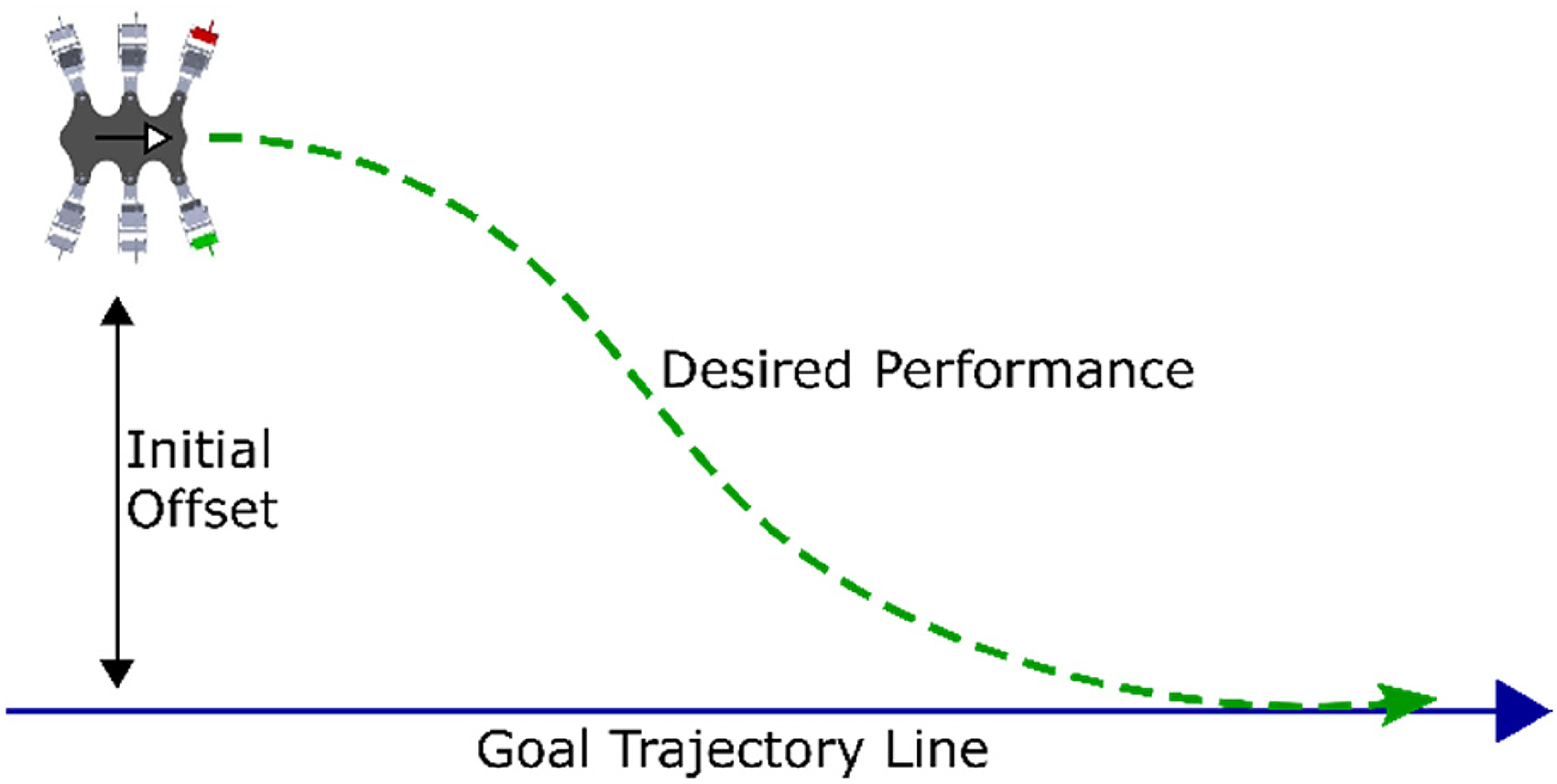
Desired hexapod trajectory tracking behavior for the 18 degrees-of-freedom (DOF) hexapod (six legs and three DOF per leg).

Action space and central pattern generator

The action space of the hexapod control system uses a CPG in combination with a set of mapping functions to produce smooth joint angle signals while offering precise control over the motion. The oscillators and mapping functions described by Wang et al.²⁹ for use with a genetic optimization algorithm are extended in this work to function with an RL agent.

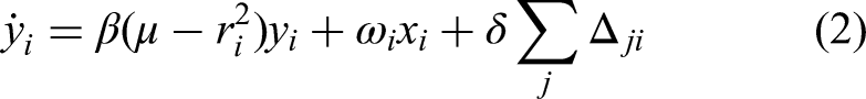
The CPG consists of six coupled Hopf oscillators, which, through the adjustment of their parameters, offer control over the amplitude, frequency, and phase angle between the hexapod's six legs. The Hopf oscillator is a proven basis for central pattern generation applied to hexapod robots.^9,14,29,30 Each leg of the robot is controlled by an individual oscillator, and the inter-oscillator coupling determines the phase differences between the hexapod's legs. Each of the six coupled Hopf oscillators is described by the following equations^9,29:

{\dot{x}}_{i} = α (μ - r_{i}^{2}) x_{i} - ω_{i} y_{i}

(1)

{\dot{y}}_{i} = β (μ - r_{i}^{2}) y_{i} + ω_{i} x_{i} + δ \sum_{j} Δ_{j i}

(2)

Δ_{j i} = y_{j} \cos (θ_{j}^{i}) - x_{j} \sin (θ_{j}^{i})

(3)

where x and y are the oscillator state variables, ω is the frequency,

\sqrt{μ}

is the amplitude, and β is the convergence velocity. The subscripts i and j indicate the oscillator/leg numbers (between 1 and 6). The parameters dealing with the oscillator coupling are the coupling strength between oscillators δ, the coupling value

Δ_{j i}

, and the phase angle

θ_{j}^{i}

between oscillator i and oscillator j. Wang et al.²⁹ implement fully-symmetric bidirectional coupling between the six oscillators; however, it was found in the present research that using a leader oscillator and five followers also produces the desired result. In this work, one of the oscillators is selected to be the leader, and the phase angles for the remaining five oscillators are referenced to the leader.

Mapping functions are used to transform the Hopf oscillator x and y signals into joint angle signals for each of the hexapod's 18 DOF. There are six sets of mapping functions (one for each individual leg). The mapping functions take the state variables x and y from the Hopf oscillator and convert them into three angle signals for the hip, knee, and ankle joints of the corresponding leg. The mapping functions presented by Wang et al.²⁹ utilize piecewise functions for both the knee and ankle angles to differentiate between the swing and stance phases of the leg motion. In the present work, these piecewise functions are replaced with a single function for all conditions, as the RL agent should be able to infer when each leg is in a swing or stance phase from the provided observations, and the agent can also adjust the mapping function parameters in reaction to external stimuli. The mapping functions corresponding to each Hopf oscillator are as follows:

θ_{1, i} = k_{0, i} y_{i}

(4)

θ_{2, i} = k_{1, i} x_{i} + b_{1, i}

(5)

θ_{3, i} = k_{2, i} θ_{2, i} + b_{2, i}

(6)

where the subscript i indicates the oscillator/leg number,

θ_{1, i}

indicates the hip angle for leg i,

θ_{2, i}

is the knee angle for leg i, and

θ_{3, i}

is the ankle angle for leg i. For each leg i, parameters

k_{0, i}

k_{1, i}

, and

k_{2, i}

are proportionality factors, while

b_{1, i}

and

b_{2, i}

are bias values in the mapping functions which can be adjusted to modify the base gait. The proportionality factors and the biases are the means through which the RL agent controls the motion of the hexapod. With five parameters per leg, and six legs, the resulting set of 30 parameters forms the action space of the RL agent.

Observations

The observations considered in this research utilize sensors that are internal to the hexapod robot, meaning that the hexapod could be operated in an unstructured environment. There are some observations which are always used and are, therefore, not included as “factors” in the designed experiment. These observations are considered essential for achieving the desired performance of the hexapod or are readily accessible without the need for additional sensors.

The observations that are included in all the designed experiment runs are the joint angles (3 joint angles per leg × 6 legs = 18 joints), the joint angular velocities (18 joints), the Hopf oscillator x and y parameters (x and y parameters × 6 coupled oscillator = 12), the previous time step actions (30 parameters in the action space), and the offset from the goal trajectory line (one distance measurement).

The observations (and associated number of measurement signals) which are used as “factors” in the designed experiment to study their relative effect on RL performance are the joint torques (18 joints), the body linear velocities (three axes), the body orientation (four parameters in the form of a quaternion), the body angular velocities (three axes), the body height above the ground (one distance measurement), the magnitudes of the leg tip ground contact forces (6 normal + 6 frictional = 12 forces), and the leg tip ground contact binary signals (6 leg tip contacts, +1 if contact, 0 if no contact). All observations are normalized to lie between ±1 before being passed to the neural network.

The reward function

The reward function is designed to train the hexapod to follow the desired trajectory line. The reward function contains positive reward terms to encourage positive actions, and negative reward terms to discourage undesirable actions. The total reward is calculated as shown in equation (7), with the individual reward terms detailed in Table 2. Note that the C parameters in Table 2 correspond to reward term scale factors.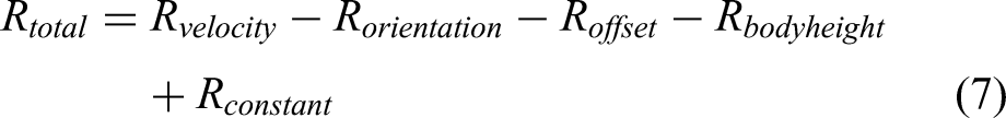

R_{t o t a l} = R_{v e l o c i t y} - R_{o r i e n t a t i o n} - R_{o f f s e t} - R_{b o d y h e i g h t} + R_{c o n s t a n t}

(7)

Table 2.

Detailed breakdown of reward function terms.

Reward term	Equation
Forward velocity	$R_{v e l o c i t y} = C_{1} v_{x}$
Body orientation	$R_{o r i e n t a t i o n} = C_{2} (θ_{p i t c h}^{2} + θ_{r o l l}^{2} + θ_{y a w}^{2})$
Offset from goal trajectory line	$R_{o f f s e t} = C_{3} \| Δ z \|$
Body height above ground	$R_{b o d y h e i g h t} = C_{4} (h - h_{d e s i r e d})^{2}$
Constant term	$R_{c o n s t a n t} = C_{5} \frac{t_{s}}{t_{f}}$

The reward function terms were chosen in order to achieve the path trajectory following goal. The forward velocity and offset from the goal trajectory line terms directly reward the hexapod for the desired behavior. The body orientation and body height penalties provide additional feedback to help produce a gait with a smoother motion of the hexapod body, which could be carrying a payload and/or sensors during deployment. The constant term added to the reward function helps the RL agent at the start of training to encourage the agent to utilize the entire training episode without triggering an early termination (due to, for example, flipping upside down to avoid future penalties). The reward term scale factors are of similar magnitude and were determined through manual tuning and remain fixed for the entirety of this work. While changing the weighting of the reward terms can affect the resulting performance of the hexapod, in this work, the decision was made to focus the designed experiments on the selection of observations while keeping the reward function fixed.

The RL agent

The hexapod is controlled by an RL agent trained using DDPG,³¹ which has been proven effective for legged robotics locomotion applications.^8,12,14,15 The actor and critic networks applied in this work utilize the same structure and size as those found in Mathworks,³² which applies RL to a quadruped robot with a similar number of observations and actions.

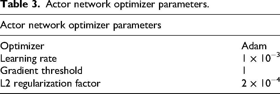
The actor network takes as input the observations from the hexapod simulation and outputs the next time step actions with the goal of maximizing hexapod performance on the trajectory following task. As shown on the left-hand side (LHS) of Figure 2, the actor network consists of an input layer for the observations, two fully connected hidden layers, and a fully connected output layer. The input layer size changes based on the number of observations used in the trial, but the remaining layers maintain a fixed number of nodes. The two hidden layers and output layer have 400, 300, and 30 nodes, respectively. The hidden layers utilize a rectified linear unit (ReLU) activation function, while the output layer uses a hyperbolic tangent activation function to produce the 30 actions with values constrained between ±1. The optimizer parameters set in the MATLAB simulation driving script for the actor network are listed in Table 3.

Figure 2.

Actor (LHS) and critic (RHS) network flowchart representation.

Table 3.

Actor network optimizer parameters.

Actor network optimizer parameters
Optimizer	Adam
Learning rate	1 × 10⁻³
Gradient threshold	1
L2 regularization factor	2 × 10⁻⁴

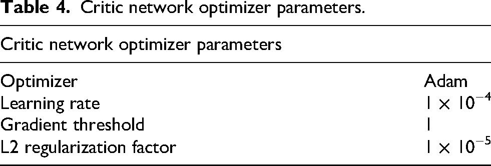
The critic network takes as input the observations from the hexapod simulation and the action signals produced by the actor network, and outputs the expected reward that will be obtained using the given actions. As shown on the RHS of Figure 2, the critic network consists of two initially separate branches that merge to produce a single output. The first branch has an input layer of the observations, followed by two fully connected hidden layers of 400 and 300 nodes. The second branch takes as input the 30 actions from the actor network and has a fully connected hidden layer of 300 nodes. Both branches of the network are connected with an additional layer that appends the two branches into a single layer of 600 nodes. Following this layer is a fully connected layer of a single node, which produces the critic output. All hidden layers use ReLU activation functions, while the final output layer does not have any activation function to generate the critic output. The optimizer parameters set in the MATLAB simulation driving script for the critic network are listed in Table 4.

Table 4.

Critic network optimizer parameters.

Critic network optimizer parameters
Optimizer	Adam
Learning rate	1 × 10⁻⁴
Gradient threshold	1
L2 regularization factor	1 × 10⁻⁵

RL training routine

Each RL training routine consists of 1000 individual episodes. Each episode lasts 15 seconds. The RL training hyperparameters are shown in Table 5. These values were determined by starting with the values used in Mathworks,³² and then fine-tuning them by hand before completing the designed experiment study. The parameters in Tables 3 to 5 remained fixed throughout the designed experiments.

Table 5.

DDPG learning hyperparameters set in the driving routine.

Reinforcement learning training hyperparameters
Number of episodes	1000
Sample time (s)	0.03
Discount factor	0.99
Mini batch size	250
Experience buffer length	1 × 10⁶
Target smoothing factor	1 × 10⁻³
Noise mean attraction constant	0.15
Noise standard deviation	0.1

The designed experiment

The observations which are varied in the designed experiment (called factors) are given an indicator letter as follows: joint torques (A), body linear velocities (B), body orientation in the form of a quaternion (C), body angular velocities (D), body height from the ground plane (E), magnitudes of the leg tip ground contact forces (normal and frictional) (F), and leg tip ground contact binary signals (G). The seven possible observations each have the option of being on or off (used for learning or not); therefore, they are two-level factors.

Seven two-level factors lead to 128 possible unique combinations from which an optimal set of observations for the given locomotion task can be selected. In addition, due to the inherently-random nature of RL, multiple repetitions (called replicants) of each case were carried out to help distinguish between the performance of different combinations of observations. For this work, 10 replicants were selected for each case to help ensure that there is a statistical significance when comparing learning results.

A quarter-fraction factorial designed experiment was tested, which consists of 32 separate cases to be run. This number is significantly lower than the 128 required for the full factorial designed experiment. With 32 cases for the quarter fraction designed experiment and 10 replicants per case, a total of 320 separate RL runs were needed. The quarter-fraction factorial design was selected as it is an IV resolution design where no main factors are aliased with any first-order interactions. As sensor measurements on the hexapod can be physically related (e.g. ground contact of the feet can affect the body tilt), it is desirable that no interactions are confounded with any of the main effects. The design generators for the quarter-fraction experiment using the principal fraction are $F = A B C D$ and $G = A B D E$ .

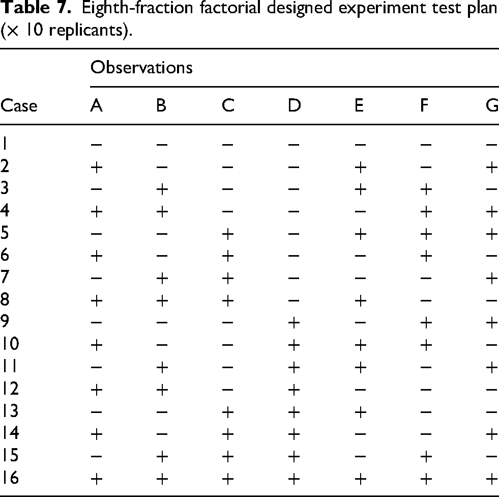
An eighth-fraction factorial design was also tested to determine if the number of cases to run could further be reduced to 16 while still maintaining a suitable level of accuracy. The IV resolution eighth-fraction design has generators: $E = A B C$ , $F = B C D$ , and $G = A C D$ .

Both factorial designs were set up using the Minitab statistical software.³³ Tables 6 and 7 show the design table for the experiments generated using Minitab, where each case was repeated for 10 replicants to account for the random nature of RL. A plus sign in the tables indicates that the observation will be used for the specific case, while a negative sign shows when the observation is turned off. The only changes to the hexapod simulation throughout this study are the set of observations used (according to Tables 6 and 7), which, in turn, affects the number of nodes in the input layer of both the actor and critic networks. All other aspects of the simulation remain fixed.

Table 6.

Quarter-fraction factorial designed experiment test plan (× 10 replicants).

Case	Observations
Case	A	B	C	D	E	F	G
1	−	−	−	−	−	+	+
2	+	−	−	−	−	−	−
3	−	+	−	−	−	−	−
4	+	+	−	−	−	+	+
5	−	−	+	−	−	−	+
6	+	−	+	−	−	+	−
7	−	+	+	−	−	+	−
8	+	+	+	−	−	−	+
9	−	−	−	+	−	−	−
10	+	−	−	+	−	+	+
11	−	+	−	+	−	+	+
12	+	+	−	+	−	−	−
13	−	−	+	+	−	+	−
14	+	−	+	+	−	−	+
15	−	+	+	+	−	−	+
16	+	+	+	+	−	+	−
17	−	−	−	−	+	+	−
18	+	−	−	−	+	−	+
19	−	+	−	−	+	−	+
20	+	+	−	−	+	+	−
21	−	−	+	−	+	−	−
22	+	−	+	−	+	+	+
23	−	+	+	−	+	+	+
24	+	+	+	−	+	−	−
25	−	−	−	+	+	−	+
26	+	−	−	+	+	+	−
27	−	+	−	+	+	+	−
28	+	+	−	+	+	−	+
29	−	−	+	+	+	+	+
30	+	−	+	+	+	−	−
31	−	+	+	+	+	−	−
32	+	+	+	+	+	+	+

Table 7.

Eighth-fraction factorial designed experiment test plan (× 10 replicants).

Case	Observations
Case	A	B	C	D	E	F	G
1	−	−	−	−	−	−	−
2	+	−	−	−	+	−	+
3	−	+	−	−	+	+	−
4	+	+	−	−	−	+	+
5	−	−	+	−	+	+	+
6	+	−	+	−	−	+	−
7	−	+	+	−	−	−	+
8	+	+	+	−	+	−	−
9	−	−	−	+	−	+	+
10	+	−	−	+	+	+	−
11	−	+	−	+	+	−	+
12	+	+	−	+	−	−	−
13	−	−	+	+	+	−	−
14	+	−	+	+	−	−	+
15	−	+	+	+	−	+	−
16	+	+	+	+	+	+	+

The recorded performance metric used as the response in the analysis of the designed experiments is the final average reward at 1000 training episodes. This performance metric was selected because after 1000 episodes, the learning of the RL agent has generally plateaued, and the agent has reached its maximum potential for the given set of observations. When training in simulation to deploy on physical hardware, the final performance of the RL agent was considered more important than its learning speed, so 1000 episodes were used to ensure the RL agent could reach its peak performance.

Analysis of results

This section presents and analyzes the results of the designed experiments. Detailed step-by-step analysis of the quarter-fraction factorial designed experiment data is presented in this section, with the analysis of the eighth-fraction experiment following an identical procedure. Using the gathered data, a regression model is formulated to model how the observations affect the hexapod performance. This model is then used to predict which combination of observations yields the highest rewards during training. The metric used to evaluate the performance of the RL agent using different observations is the final average reward after training for 1000 episodes. The model predictions and corresponding trained agent are then validated within the developed hexapod simulator.

To evaluate the regression model fit, the following three R² statistics are used. 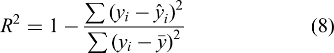$R^{2}$ quantifies the fit of the model and produces a value between 0 and 1, which indicates the percentage of variability in the data which is accounted for by the model, where the larger the value, the better the fit. This $R^{2}$ statistic is calculated as follows³⁴:

R^{2} = 1 - \frac{\sum {(y_{i} - {\hat{y}}_{i})}^{2}}{\sum {(y_{i} - \bar{y})}^{2}}

(8)

where

y_{i}

represents the final average reward obtained for the ith test case during the designed experiment,

{\hat{y}}_{i}

is the final average reward predicted by the model for the given case i, and

\bar{y}

is the mean of all final average rewards in the designed experiment dataset. This statistic, however, does not account for model size/complexity in quantifying the performance of the model.

The adjusted statistic 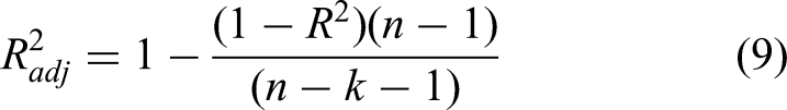$R_{a d j}^{2}$ encourages a simple model and is calculated as follows:

R_{a d j}^{2} = 1 - \frac{(1 - R^{2}) (n - 1)}{(n - k - 1)}

(9)

where

R^{2}

is the R² statistic from equation (8), n is the number of datapoints in the experimental dataset, and k represents the number of independent variables in the regression model.

The third statistic is the predicted R² value 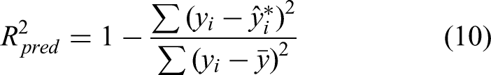$R_{p r e d}^{2}$ , which compares the fit of different models to help detect overfitting of the model and is a measure of how well a regression model predicts responses for new observations. This statistic is calculated as follows:

R_{p r e d}^{2} = 1 - \frac{\sum {(y_{i} - {\hat{y}}_{i} *)}^{2}}{\sum {(y_{i} - \bar{y})}^{2}}

(10)

where

{\hat{y}}_{i} *

represents the predicted final average reward for the ith case, obtained using a model that is fit to the dataset after systematically removing the experiment run to be predicted.

R_{p r e d}^{2}

will always be less than

R^{2}

because of the removal of each data point during the calculation, but an

R_{p r e d}^{2}

that is significantly smaller than

R^{2}

can be a warning sign of overfitting.

The resulting learning curves for each of the 10 replicants for a given case (corresponding to a particular combination of observations) can be plotted together on a single graph to visualize the repeatability of the learning process. Figure 3 shows the 10 replicants for case 5 of the quarter-fraction experiment as a representative example. The moving average reward curves are plotted as a function of training episode and shown in Figure 3 as black lines. An overall average reward curve is shown by the thicker red line. Figure 3 shows that, for case 5, eight out of the 10 replicants follow a very similar learning curve, while two of the replicants failed to learn and appear as outliers in the data. A similar spread of learning curves and outliers obtained for multiple repetitions of the same DDPG learning process were also observed by Naya et al.¹⁵ and Schilling et al.²¹ The learning routine includes several randomized processes, such as initialization of neural network weights and biases, as well as noise artificially introduced for exploration of the possible action space. As a result of the stochastic nature of RL, some outliers in the data are inevitable.

Figure 3.

Learning curves for all 10 replicants of case 5.

Table 8 summarizes the results of the quarter-fraction designed experiment showing, for each case, the average final reward of 10 replicants. Referring to this table, it is interesting to note that using the maximum number of observations (case 32) does not achieve the highest learning performance. Case 32 (which contains all seven observations) yielded an average final reward over 10 replicants, which is lower than cases 6, 8, 14, 16, 21, 22, 28, 30, and 31 (which all contain different combinations of fewer than seven observations).

Table 8.

Summary of results of the one-quarter fraction designed experiment.

Case	Observations							Average final reward over 10 replicants
Case	A	B	C	D	E	F	G	Average final reward over 10 replicants
1	−	−	−	−	−	+	+	−8048
2	+	−	−	−	−	−	−	−7384
3	−	+	−	−	−	−	−	−3500
4	+	+	−	−	−	+	+	−6764
5	−	−	+	−	−	−	+	−2433
6	+	−	+	−	−	+	−	−1752
7	−	+	+	−	−	+	−	−2489
8	+	+	+	−	−	−	+	−1392
9	−	−	−	+	−	−	−	−6198
10	+	−	−	+	−	+	+	−10328
11	−	+	−	+	−	+	+	−4704
12	+	+	−	+	−	−	−	−5369
13	−	−	+	+	−	+	−	−2226
14	+	−	+	+	−	−	+	−1265
15	−	+	+	+	−	−	+	−2002
16	+	+	+	+	−	+	−	−1692
17	−	−	−	−	+	+	−	−7664
18	+	−	−	−	+	−	+	−5956
19	−	+	−	−	+	−	+	−6855
20	+	+	−	−	+	+	−	−1957
21	−	−	+	−	+	−	−	−630
22	+	−	+	−	+	+	+	−773
23	−	+	+	−	+	+	+	−2364
24	+	+	+	−	+	−	−	−2014
25	−	−	−	+	+	−	+	−7748
26	+	−	−	+	+	+	−	−4675
27	−	+	−	+	+	+	−	−4982
28	+	+	−	+	+	−	+	−1224
29	−	−	+	+	+	+	+	−2658
30	+	−	+	+	+	−	−	−1414
31	−	+	+	+	+	−	−	−579
32	+	+	+	+	+	+	+	−1776

Cases with rewards in bold font have average final rewards that are higher than case 32 (which contains all seven observations).

A regression model was fit to the data to model how the seven studied observations affect the hexapod performance. As the designed experiment featured 32 separate cases, the regression model can have a maximum of 32 terms. The fit of the regression model is evaluated using R² values as well as studying the distribution of the model residuals.

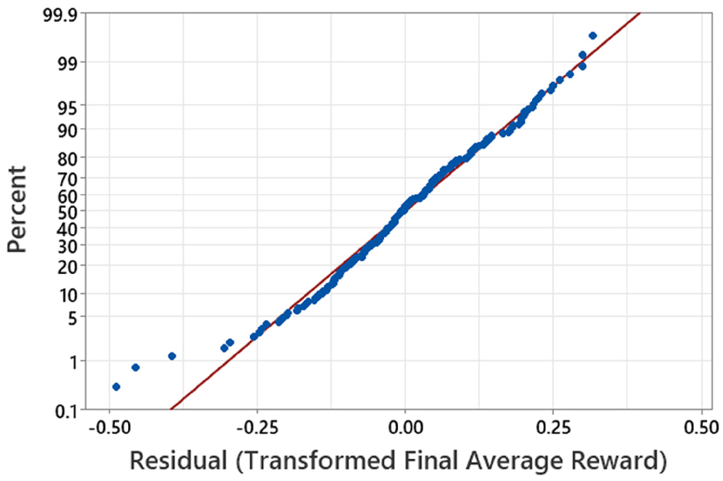
The model residuals for the initial fit can be illustrated using a histogram plot as shown in Figure 4. The residuals are grouped into 20 bins of equal width over the total range of average final reward values, with the frequency in each bin shown on the vertical y-axis. Figure 4 clearly shows that the initial regression model generated in Minitab is not a good fit to the final reward data since, instead of a zero-mean normal distribution, the residuals’ distribution is skewed to the left and the peak of the distribution is shifted to the right of zero.

Figure 4.

Histogram of residuals for the initial model fit.

Three steps were taken to improve the model fit and produce the final regression model. First, the worst three replicants of each run were removed from the analysis to eliminate the worst outliers. Fitting the model to the best seven replicants of each run effectively removed the long tail on the LHS of the residual distribution and centered the residuals about zero as desired.

Given that the goal of this research is to explore the potential for the application of a designed experiment in the selection of observations for deployment on a physical robot hexapod, it is reasonable to remove outlying replicants because, in a deployment scenario, only the best RL agents would be considered for the hexapod from multiple learning routines.

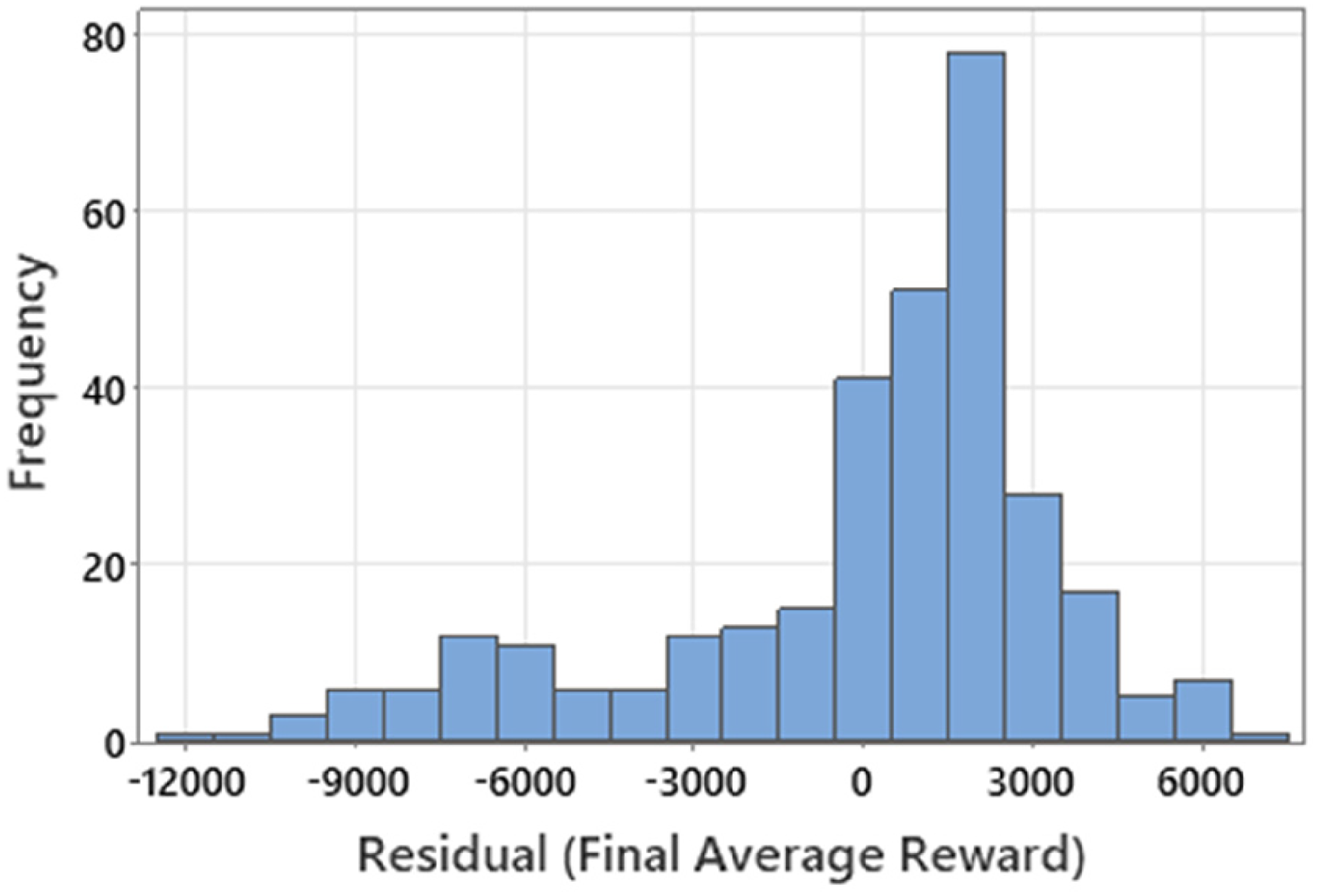
Next, the final average rewards were transformed using the following nonlinear transformation to further improve the model fit:

Y^{'} = e^{\frac{Y}{7500}}

(11)

where Y is the final average reward and

Y^{'}

is the resulting transformed response. The scaling factor in this transformation was determined empirically using an iterative approach to maximize the

R^{2}

value of the model fit to the transformed data, similar to the approach used by Pardoe et al.³⁴

Finally, the 32-term model was reduced to 13 terms by eliminating interaction terms having less than a 5% significance to arrive at the final regression model. The histogram of residuals for the final model is shown in Figure 5. This histogram displays a wide peak centered around zero, which shows that the model is a good fit to many of the experimental data points. There are only three residuals skewing the LHS of the distribution, which would be expected from runs with combinations of observations that result in inconsistent and poor learning.

Figure 5.

Histogram of residuals for the final model.

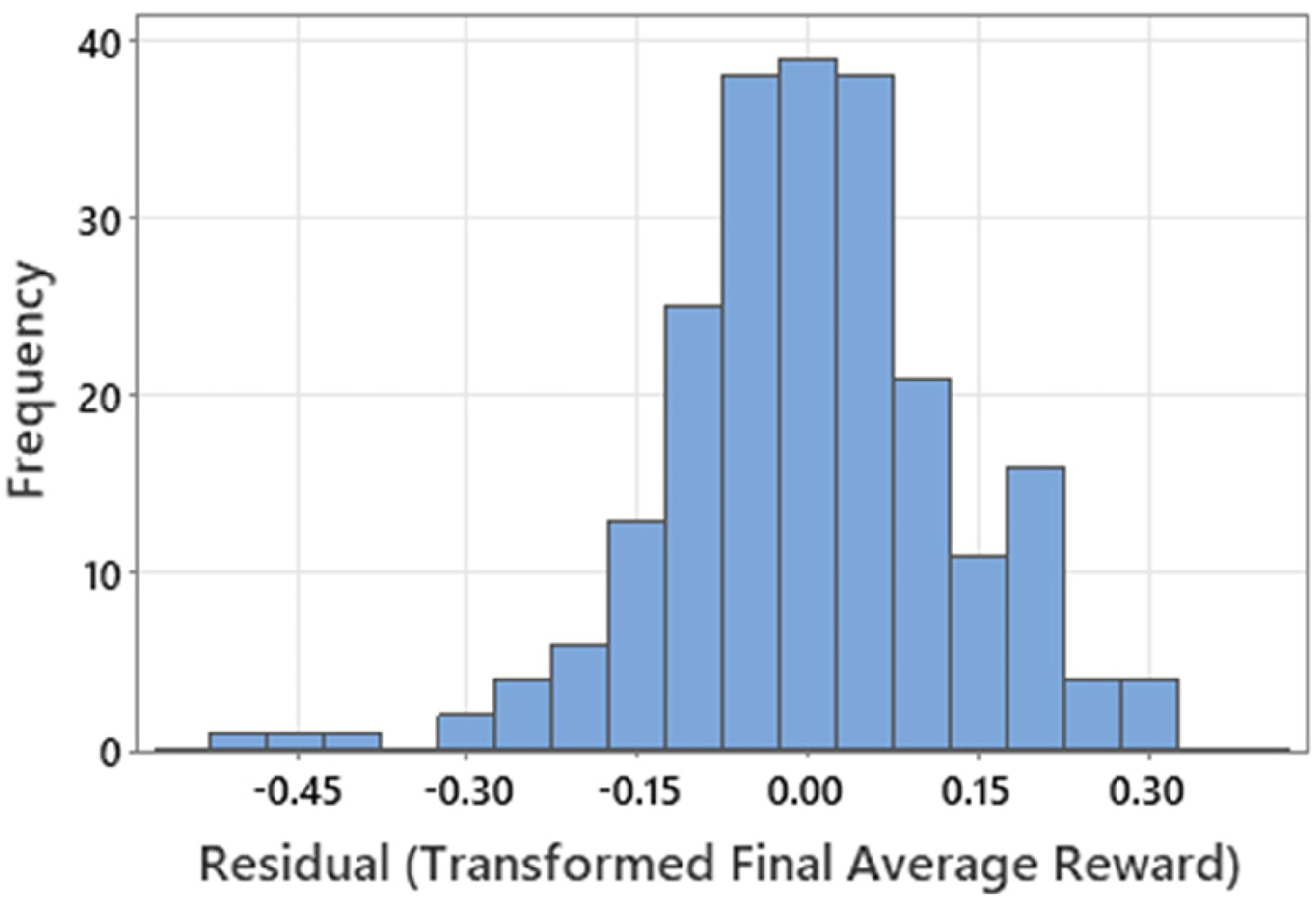
The residuals of the final model are also plotted on a normal probability plot as shown in Figure 6. A normal probability plot shows how the experimental data differs from the desired normal distribution by illustrating deviations from the diagonal red line (where the red line represents a random normal distribution). It can be seen in Figure 6 that the blue residuals closely follow a normal distribution, confirming the successful fit of the final model.

Figure 6.

Normal probability plot for the final model.

Table 9 summarizes how the $R^{2}$ , $R_{a d j}^{2}$ , and $R_{p r e d}^{2}$ values changed with each step in the model refinement. It can be seen from this table that the most significant improvement in model accuracy was obtained by eliminating the three worst replicants from each run, as all three R² values more than doubled. Applying the nonlinear transformation to the final average reward data further increased all three R² values by 5%–7%. Finally, reducing the model helped to reduce overfitting, as illustrated by the reduction in $R^{2}$ and $R_{a d j}^{2}$ , while showing an increase in $R_{p r e d}^{2}$ . The reduced model is better generalized to make more accurate predictions of unseen circumstances as demonstrated by the increase in $R_{p r e d}^{2}$ . Achieving higher R² values would likely be difficult for this application because of the stochastic nature of the RL process, since the random noise introduced during the learning process is difficult to model.

Table 9.

Improvement in model fit with each key step in the analysis.

Model description	$R^{2}$	$R_{a d j}^{2}$	$R_{p r e d}^{2}$
Initial model	35 %	28 %	20 %
Best 7 replicants model	73 %	68 %	63 %
Model using transformed data	77 %	74 %	69 %
Final reduced model	75 %	73 %	72 %

The final regression model determined using the quarter-fraction experiment design is given by equation (12), where each letter would be replaced with either the number 1 if the observation is present, or −1 if the observation is turned off.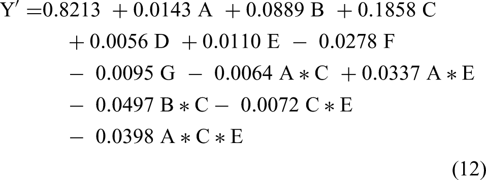

\begin{aligned} Y^{'} = & 0.8213 + 0.0143 A + 0.0889 B + 0.1858 C \\ + 0.0056 D + 0.0110 E - 0.0278 F \\ - 0.0095 G - 0.0064 A * C + 0.0337 A * E \\ - 0.0497 B * C - 0.0072 C * E \\ - 0.0398 A * C * E \end{aligned}

(12)

The resulting data generated through the quarter-fraction designed experiment can be compared to that from the eighth-fraction experiment. Figure 7 shows the mean effect of each observation calculated from the data of both designed experiments, along with the associated standard errors. The mean of all experimental runs, which both included and excluded each given observation are plotted to show the average effect of the observation. Figure 7 demonstrates how the mean effects captured in the experimental data are comparable for both quarter and eighth fraction designed experiments, as they have overlapping error bars for all seven observations—an indication that even 16 runs can be sufficient to model the effects of the observations. As can be seen in the figure, for the simulation conditions used in this work, the body orientation (observation C) proved to be the most important factor for maximizing hexapod performance.

Figure 7.

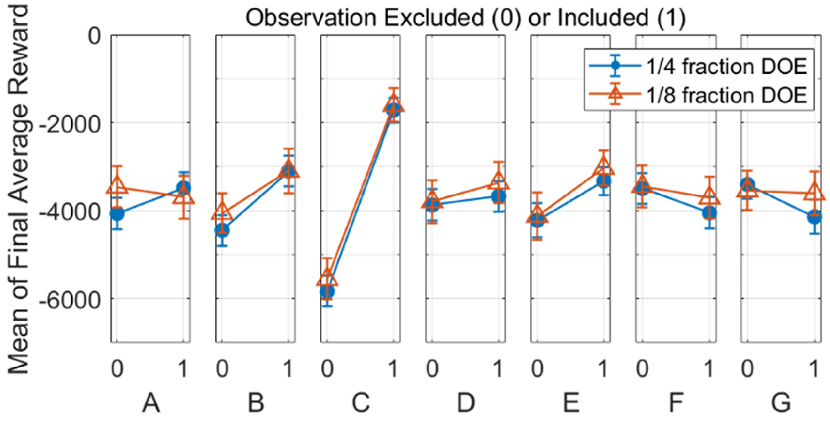
Mean effect of observations on the final average reward as calculated from the 1/4 and 1/8 fraction experiments’ data.

Through an identical analysis method to that previously described for the quarter-fraction experiment data, the regression given by equation (13) can be determined from the data of the eighth-fraction designed experiment.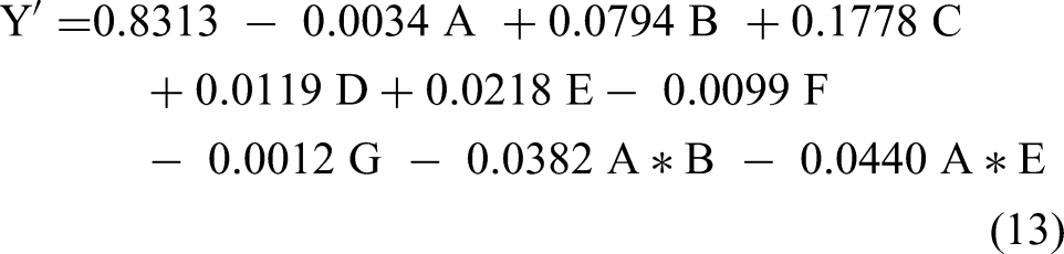

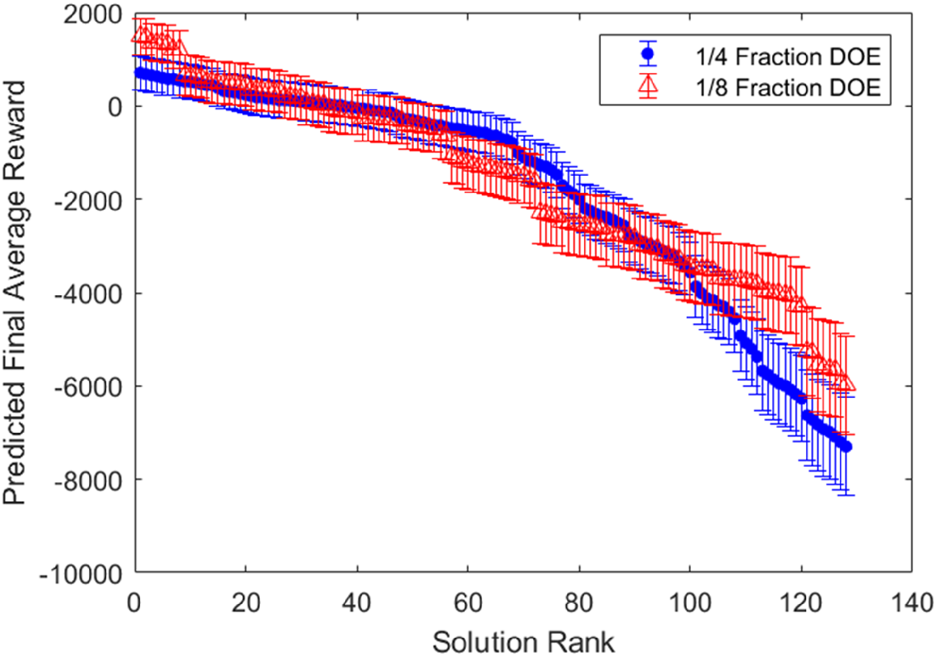
\begin{aligned} Y^{'} = & 0.8313 - 0.0034 A + 0.0794 B + 0.1778 C \\ + 0.0119 D + 0.0218 E - 0.0099 F \\ - 0.0012 G - 0.0382 A * B - 0.0440 A * E \end{aligned}

(13)

Both models from equations (12) and (13) are then used to predict the hexapod performance for all 128 possible combinations of observations from the small subsets tested in the designed experiments. Figure 8 shows the predicted final average rewards for all combinations in order of performance with the associated 90% confidence intervals in the predictions. Figure 8 shows that the predictions from both the quarter (blue dots) and eighth (red triangles) fraction designed experiments have overlapping 90% confidence intervals across the entire range of performance. Combinations of observations that are close in ranked performance have overlapping confidence intervals due to the stochastic nature of RL. If tested, one could expect that any given combination of observations could change in ranking based on the overlap with nearby confidence intervals. In practice, one might test the top 5 to 10 predicted combinations and select the final set of observations based on these validation tests.

Figure 8.

Predicted final average reward for all 128 combinations of factors in order of performance with associated 90% confidence intervals.

The three highest-ranked solutions that were predicted by the quarter-fraction model were tested in the simulation environment to validate the results. These solutions are summarized in Table 10 and correspond to the three highest predicted final average rewards on the LHS of Figure 8.

Table 10.

Summary of the three highest-ranked solutions predicted by the ¼ fraction experiment model with associated 90% confidence intervals.

Highest-ranked solutions	Factors							Final average reward
Highest-ranked solutions	A	B	C	D	E	F	G	Prediction	90% confidence interval
1	+	+	+	+	−	−	−	711	(343, 1061)
2	+	+	+	+	+	−	−	681	(311, 1032)
3	−	+	+	+	+	−	−	656	(285, 1009)

When tested, all three solutions achieved final average rewards within the predicted confidence intervals. During this validation testing, the second solution achieved the highest reward of all cases completed in this work, without being a part of the initial cases from the designed experiment. Since the confidence intervals are overlapping between adjacent solutions, and the learning results will always contain some level of noise, any one of the top three solutions could have produced the highest average final reward—in this instance, it was solution #2. These results demonstrate that a designed experiment could potentially be a valuable tool when selecting and optimizing the observations needed for a hexapod locomotion problem. Based on these validation tests, for the conditions used in this research, the observations achieving the highest average reward correspond to solution #2 as follows: the joint torques (A), body linear velocities (B), body orientation (C), body angular velocities (D), and body height (E).

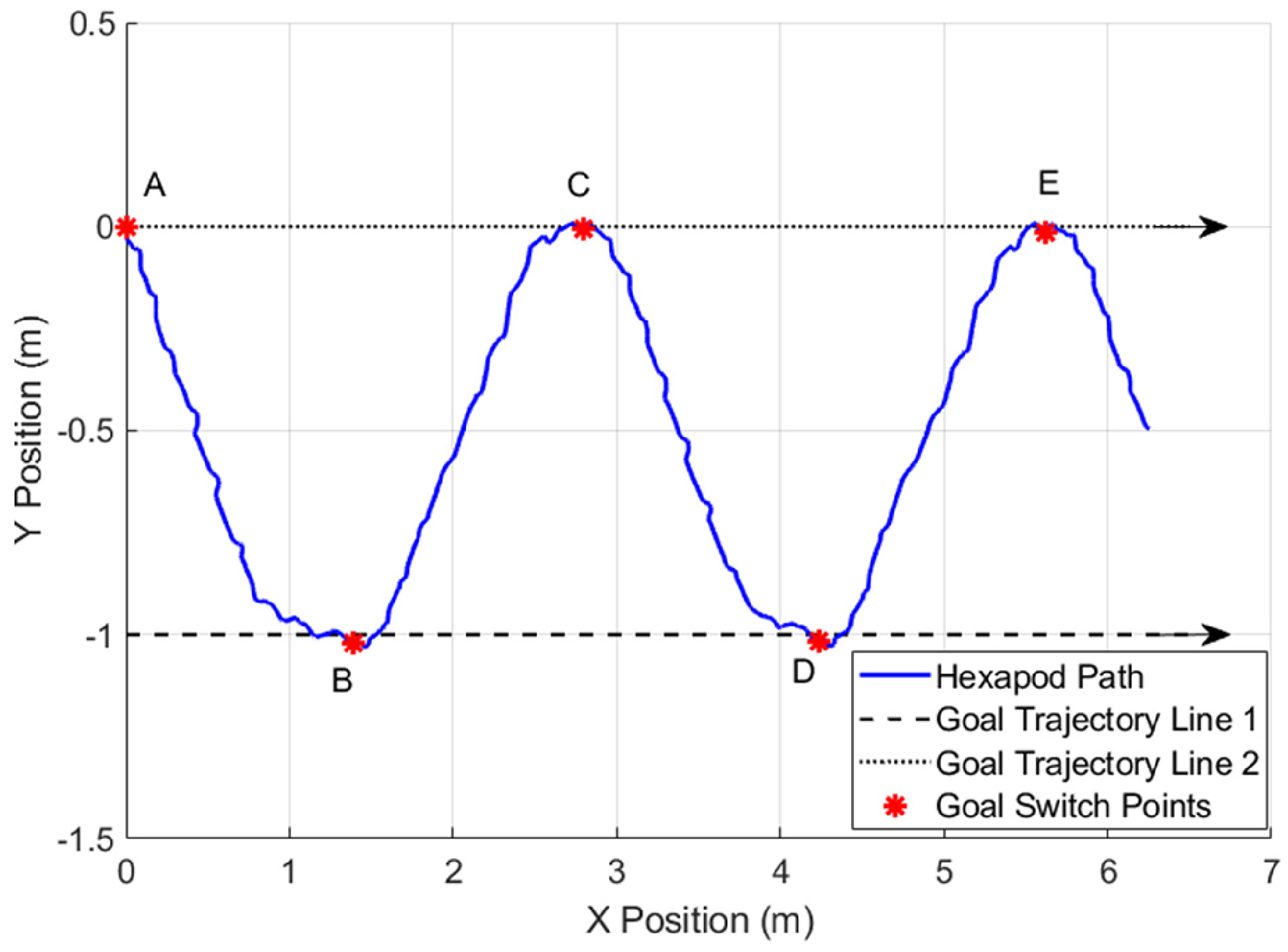
Finally, the trained RL agent was deployed within the simulator to demonstrate the ability of the hexapod to follow a moving goal trajectory line. Figure 9 shows a top-down view of this case study in the x–y plane, where the goal trajectory line alternates at regular intervals between $y = - 1$ m and $y = 0$ m, corresponding to Goal Trajectory Line 1 and Goal Trajectory Line 2, respectively. The path followed by the hexapod is shown by a blue line. It can be seen in this figure that the hexapod is able to move between the two goal trajectory lines, resulting in a sinusoidal path. The red points along the hexapod's path indicate the moment that the goal trajectory line switched positions. For example, when the hexapod reached points A, C, and E, the goal was set to Trajectory Line 1. Similarly, when the hexapod reached points B and D, the goal was set to Trajectory Line 2. This scenario is analogous to the hexapod circumventing obstacles while moving along the x-direction.

Figure 9.

Hexapod trajectory following task.

Conclusions

A thorough examination and survey of the current literature related to RL applied to hexapod robots revealed a wide range of RL agent observations, without a clear method of justification for these choices. The observations provided to the RL agent are important because they affect hexapod performance, hardware cost, power requirements, and computational load. This work presented the use of fractional factorial designed experiments as a tool to aid in the selection of observations.

A hexapod simulator was developed using a CPG control scheme consisting of six coupled Hopf oscillators and associated mapping functions. Quarter-fraction and eighth-fraction factorial designed experiments were carried out using the hexapod simulator to explore the effect of seven potential observations on the hexapod's walking performance.

The factorial designed experiments were able to generate regression models that provided insight into the seven studied observations. For the conditions used in this research, the observations that obtained the maximum final average reward correspond to the joint torques, body linear velocities, body orientation, body angular velocities, and body height.

Further research should be conducted to explore this potential. Recommended areas of future research include exploring the application of this methodology for selecting observations of different RL algorithms, such as proximal policy optimization or soft actor-critic. The effect on performance of the weighting of terms in the reward function could also potentially be explored using a designed experiment, using the reward term scale factors as the factors of the designed experiment. Finally, since optimal observations may differ between tasks for the same hexapod, the use of a designed experiment for observation optimization could be further studied by modifying the simulator environment to test the hexapod in a variety of scenarios, such as traversing rough terrain, climbing stairs, transporting a payload, or walking with a damaged leg.

Footnotes

Acknowledgments

Not applicable.

ORCID iDs

Alec Freeman

Robert Bauer

Ethical considerations

Ethical approval was not required.

Consent to participate

Not applicable.

Consent for publication

Not applicable.

Funding

The authors disclosed receipt of the following financial support for the research, authorship, and/or publication of this article: The authors received financial support from the Natural Sciences and Engineering Research Council of Canada (NSERC) (grant number 07025-2020).

Declaration of conflicting interests

The authors declared no potential conflicts of interest with respect to the research, authorship, and/or publication of this article.

Data availability statement

Not applicable.

References

Coelho

Ribeiro

Dias

, et al. Trends in the control of hexapod robots: a survey. Robotics 2021; 10: 00.

Rubio

Valero

Llopis-Albert

. A review of mobile robots: concepts, methods, theoretical framework, and applications. Int J Adv Robot Syst 2019; 16: 1729881419839596.

Ibarz

Tan

Fin

, et al. How to train your robot with deep reinforcement learning: lessons we have learned. Int J Robot Res 2021; 40: 698–721.

Clarke

Kempson

. Introduction to the design and analysis of experiments. London, UK: Arnold, 1997.

Heess

Lemmon

, et al. Emergence of locomotion behaviours in rich environments. http://arxiv.org/abs/1707.02286 (2017, accessed 22 July 2025).

Yang

Gao

. Terrain-adaptive central pattern generators with reinforcement learning for hexapod locomotion. http://arxiv.org/abs/2310.07744 (2023, accessed 22 July 2025).

Wang

Huangfu

, et al. A soft actor-critic approach for a blind walking hexapod robot with obstacle avoidance. Actuators 2023; 12: 93.

Qiu

Wei

Liu

. Adaptive gait generation for hexapod robots based on reinforcement learning and hierarchical framework. Actuators 2023; 12: 75.

Wei

Qiu

. Combined reinforcement learning and CPG algorithm to generate terrain-adaptive gait of hexapod robots. Actuators 2023; 12: 57.

10.

Liu

Sontakke

. PM-FSM: policies modulating finite state machine for robust quadrupedal locomotion. http://arxiv.org/abs/2109.12696 (2022, accessed 22 July 2025).

11.

Issa

Aldair

. Learning the quadruped robot by reinforcement learning (RL). Iraqi J Electr Electron Eng 2022; 18: 117–126.

12.

Zeng

Wang

, et al. Gait self-learning for damaged robots combining bionic inspiration and deep reinforcement learning. In: 40th Chinese Control Conference (CCC), Shanghai, China, 2021.

13.

Sun

Ling

, et al. Adaptive quadruped balance control for dynamic environments using maximum-entropy reinforcement learning. Sensors 2021; 21: 5907.

14.

Ouyang

Chi

Pang

, et al. Adaptive locomotion control of a hexapod robot via bio-inspired learning. Front Neurorobotics 2021; 15: 627157.

15.

Naya

Kutsuzawa

Owaki

, et al. Spiking neural network discovers energy-efficient hexapod motion in deep reinforcement learning. IEEE Access 2021; 9: 150345–150354.

16.

Kumar

Pathak

, et al. RMA: Rapid motor adaptation for legged robots. http://arxiv.org/abs/2107.04034 (2021, accessed 22 July 2025).

17.

Kim

Son

Lee

. Learning multiple gaits of quadruped robot using hierarchical reinforcement learning. http://arxiv.org/abs/2112.04741 (2021, accessed 22 July 2025).

18.

Liu

. Blind adaptive gait planning on non-stationary environments via continual reinforcement learning. In: IEEE International Conference on Unmanned Systems (ICUS), Beijing, China, 2021.

19.

Anne

Wilkinson

. Meta-reinforcement learning for adaptive motor control in changing robot dynamics and environments. http://arxiv.org/abs/2101.07599 (2021, accessed 22 July 2025).

20.

Verma

Nair

Agarwal

, et al. Deep reinforcement learning for single-shot diagnosis and adaptation in damaged robots. In: Proceedings of the 7th ACM IKDD CoDS and 25th COMAD, Hyderabad, India, 2020.

21.

Schilling

Konen

Ohl

, et al. Decentralized deep reinforcement learning for a distributed and adaptive locomotion controller of a hexapod robot. http://arxiv.org/abs/2005.11164 (2020, accessed 22 July 2025).

22.

Jain

Iscen

Caluwaerts

. Hierarchical reinforcement learning for quadruped locomotion. In: IEEE/RSJ International Conference on Intelligent Robots and Systems (IROS), Macau, China, 2019.

23.

Jain

Iscen

Caluwaerts

. From pixels to legs: hierarchical learning of quadruped locomotion. http://arxiv.org/abs/2011.11722 (2020, accessed 22 July 2025).

24.

Azayev

Zimmerman

. Blind hexapod locomotion in complex terrain with gait adaptation using deep reinforcement learning and classification. J Intell Robot Syst 2020; 99: 659–671.

25.

Yang

Caluwaerts

Iscen

, et al. Data efficient reinforcement learning for legged robots. http://arxiv.org/abs/1907.03613 (2019, accessed 22 July 2025).

26.

Haarnoja

Zhou

, et al. Learning to walk via deep reinforcement learning. http://arxiv.org/abs/1812.11103 (2019, accessed 22 July 2025).

27.

Iscen

Caluwaerts

Tan

, et al. Policies modulating trajectory generators. https://arxiv.org/abs/1910.02812 (2019, accessed 22 July 2025).

28.

Mathworks. Reinforcement learning agent – Simulink, 2024. https://www.mathworks.com/help/reinforcement-learning/ref/rlagent.html (accessed 22 July 2025).

29.

Wang

Cui

Sun

, et al. Parameters optimization of central pattern generators for hexapod robot based on multi-objective genetic algorithm. Int J Adv Robot Syst 2021; 18. doi:10.1177/17298814211044934

30.

Deng

Wang

Chen

, et al. CPG-inspired gait generation and transition control for six wheel-legged robot. In: China Automation Congress (CAC), Beijing, China, 2021.

31.

Lillicrap

Hunt

Pritzel

, et al. Continuous control with deep reinforcement learning. https://arxiv.org/abs/1509.02971 (2019, accessed 22 July 2025).

32.

Mathworks. Quadruped robot locomotion using DDPG agent - MATLAB & Simulink. https://www.mathworks.com/help/reinforcement-learning/ug/quadruped-robot-locomotion-using-ddpg-gent.html (2024, accessed 22 July 2025).

33.

Minitab. Data analysis, statistical & process improvement tools, Minitab. https://www.minitab.com/en-us/ (2024, accessed 22 July 2025).

34.

Pardoe

Simon

Young

. STAT 501: Regression Methods, The Pennsylvania State University. https://online.stat.psu.edu/stat501/ (2024, accessed 22 July 2025).

Factorial designed experiment to select reinforcement learning observations for a hexapod robot trajectory following task

Abstract

Keywords

Introduction

RL in hexapod control

Simulator development

Action space and central pattern generator

Observations

The reward function

The RL agent

RL training routine

The designed experiment

Analysis of results

Conclusions

Footnotes

Acknowledgments

ORCID iDs

Ethical considerations

Consent to participate

Consent for publication

Funding

Declaration of conflicting interests

Data availability statement

References