
Abstract
In the long-term deployment of mobile robots, changing appearance brings challenges for localization. When a robot travels to the same place or restarts from an existing map, global localization is needed, where place recognition provides coarse position information. For visual sensors, changing appearances such as the transition from day to night and seasonal variation can reduce the performance of a visual place recognition system. To address this problem, we propose to learn domain-unrelated features across extreme changing appearance, where a domain denotes a specific appearance condition, such as a season or a kind of weather. We use an adversarial network with two discriminators to disentangle domain-related features and domain-unrelated features from images, and the domain-unrelated features are used as descriptors in place recognition. Provided images from different domains, our network is trained in a self-supervised manner which does not require correspondences between these domains. Besides, our feature extractors are shared among all domains, making it possible to contain more appearance without increasing model complexity. Qualitative and quantitative results on two toy cases are presented to show that our network can disentangle domain-related and domain-unrelated features from given data. Experiments on three public datasets and one proposed dataset for visual place recognition are conducted to illustrate the performance of our method compared with several typical algorithms. Besides, an ablation study is designed to validate the effectiveness of the introduced discriminators in our network. Additionally, we use a four-domain dataset to verify that the network can extend to multiple domains with one model while achieving similar performance.
Introduction
Place recognition is a vital ability for robots. Ranging from autonomous driving to flying robots for precision agriculture, different kinds of sensors are leveraged in different localization scenarios, among which cameras are gaining more and more popularity. The main advantage of imagery sensors is their low cost, compared to expensive light detection and ranging (LiDAR), inertial navigation system (INS), etc. Visual localization has been studied for years, and many visual simultaneous localization and mapping (SLAM) systems are proposed, 1,2 which achieve impressive performance under ideal conditions. Visual place recognition plays two roles in a SLAM system: (1) in the mapping stage, robots need to find loop closure, so as to reduce drifting and build a global consistency map and (ii) in the localization stage, localization may sometimes fail, such as the kidnapped robot problem, which also needs loop detection. Most loop detection algorithms firstly try to coarsely relocalize the robots against a known database using place recognition, followed by pose estimation. Thus, visual place recognition may affect mapping accuracy and relocalization success rate.
As the community pays more and more attention to scenes with appearance changes, such as the urban environment, challenges for visual place recognition also come. A typical visual place recognition pipeline includes feature extraction, 3,4 feature matching, 5,6 and temporal fusion, 7,8 among which feature extraction is now a bottleneck. The recent success of deep learning has shown a great potential for a neural network to become a robust feature extractor. Thus, this article tries to improve the feature extraction module using deep learned features. The main challenge for handcrafted visual features is that they are sensitive to appearance changes, such as a shift from day to night and seasonal transitions. Some methods exploit deep learned features from supervised learning. 9,10 When testing data are similar to training data, these supervised methods perform very well. However, they require massive manually labeled data, which are labor-intensive and time-consuming. That may be unsuitable for some place recognition scenarios. Thus, self-supervised or unsupervised methods are preferred. Autoencoder learns features in a self-supervised way, and the output of the encoder is shown to be suitable for place recognition. 11 In their work, training data and testing data are quite different; therefore, it pays more attention to generalization ability. Compared to supervised learning, it sacrifices performance to obtain generalization. To find a good balance between performance and generalization, some researchers assume that training and testing data can share some similar properties, such as the same place, the same sensors, and similar illumination, but without position-level alignment. 12,13 This assumption is reasonable in some applications, such as inspection robots working in the same place at different times. ToDayGAN translated from nighttime images to daytime style using generative adversarial network (GAN), and the generated images are used to match with images captured in the daytime. 12 Although nighttime images in the training and testing phase look similar, they still have subtle appearance differences because they are captured at different times. Our article is also targeted at this setting. The main difference is that features in ToDayGAN are extracted from the translated images after the image translation, while our method directly puts constraints on features.
In this article, we are set to construct the neural network that can explicitly disentangle domain-unrelated and domain-related features of images from different domains, and the domain-unrelated features are used for place recognition. The only supervised information is the domain, where a domain denotes a specific appearance condition, such as daytime in spring or nighttime in summer. For example, by assuming that the appearance does not change too much during a short period, we can label all the images as some domain according to the appearance condition at that time. By grouping images into different domains, the proposed network can find the invariant information among them. This idea is motivated by the hypothesis that in the place recognition application, an image can be seen as the composition of place content and appearance content, where the place is the domain-unrelated content of a scene (e.g. corners or edges of buildings), whereas appearance is the domain-related properties (e.g. brightness of sunlight and type of season). Under this hypothesis, based on the definition of disentangled representation,
14
we disentangle place and appearance features using two encoders, which are part of an autoencoder. To ensure that the appearance feature only corresponds to domain-related content, an adversarial loss is applied on pairs of place features and appearance features. Besides, another adversarial loss is designed to constrain the place features mapping to the same latent space, such that the appearance feature only corresponds to domain-related information. As a result, the place feature is robust against appearance changes, and it is used as the descriptor in visual place recognition. The network is trained in a self-supervised manner without the requirement for aligned image sequences, and only domain information is needed, which is also called weak-supervised in some articles. This can be easily achieved by firstly collecting sessions of images under the same conditions and then marking each session as one domain. Besides, the network is shared across different domains, which allows our model to be adaptable to more domains without increasing the number of parameters. The main contributions of this article are listed as follows: A data modeling method is presented for visual place recognition, and a self-supervised feature learning method is proposed to disentangle the domain-unrelated and domain-related content from multiple-domain images. A disentangled feature learning network based on adversarial learning is proposed, which is able to be extended to multiples domains without increasing model complexity. This makes our network feasible for applications with limited resources. Two toy case studies are carried out to validate our feature disentanglement method with qualitative and quantitative results. We also try to interpret our network in this part. Experiments for place recognition are conducted on three public dataset and one newly proposed dataset. Our method shows favorable performance. We also open the source code for reproduction (https://github.com/dawnos/fdn-pr).
This article is an extensive study based on our previous work. 15 One additional contribution is that we improve our network to get higher performance by reconstructing high-level image feature instead of the original image. Another one is that we try to interpret our network through theoretical discussion and ablation study. Finally, more datasets and comparison methods are employed to verify the proposed disentanglement method.
The remainder of this article is organized as follows: related work is discussed and summarized in the second section. Then in the third section, we present the data model used in this article. Our method will be presented thoroughly in the fourth section. We will introduce the experiments in detail and show results in the fifth section. The conclusion will be made in the sixth section.
Related work
Typical pipeline for visual place recognition includes (1) feature extraction and (2) matching, 5,6,16 –21 optionally followed by (3) temporal fusion. 7,8,22,23 This article will focus on the feature extraction module.
Handcraft features
In the early years, handcrafted features are used for place recognition. These features can be classified into two categories, namely global features and local features. Methods based on handcrafted global features try to assign appearance-invariant features to each image directly. In some early works, histograms of oriented gradient (HOG) 24 features are used as descriptors to compute thedistance between database and query image, where the gradient is able to overcome simple illumination changes. 7 Later, the GIST descriptor, which represents the high-frequency part of an image, is also leveraged because the human eye is more sensitive to it. 25 On the other hand, local-feature-based methods firstly extract a bunch of local features and then aggregate them into global features. In place recognition, performance is limited by the choice of local features, thus local features with an appearance-invariant property are preferred. Gradient-based local features such as Scale-Invariant Feature Transform (SIFT) 3 and Oriented FAST and Rotated BRIEF Oriented FAST and Rotated BRIEF (ORB) 4 are found to be robust to small appearance changes. Especially, the ORB descriptor is used in the place recognition (loop closure) module of the widely used ORB-SLAM system. 26 In addition, different aggregating algorithms are designed to generate global descriptors, such as a bag of visual words 27 and Vector of Locally Aggregated Descriptor (VLAD). 28 Due to the limited robustness of handcrafted features, these methods are sensitive to extreme appearance changes, thus not preferable in visual place recognition.
Supervised features
After the great success of deep neural networks in the computer vision area in recent years, researchers start to explore how can visual place recognition benefit from deep learning. In one of the earliest trials, different layers in AlexNet 29 are reported to have different place recognition performances. 30 The authors find that features from the middle layers are more robust against changing appearance. However, the AlexNet features are not good enough, because the network is pretrained on the imagenet large-scale visual recognition challenge dataset, 31 which is different from the testing set. 11 To go further, different supervised methods are proposed, which constrain the extracted features of images from the same place to be similar. 9,10,32 –35 One way is to use a classification network for place recognition where each place is a class, and this method can achieve comparable results. 9 The network is trained and tested on a dataset captured from static cameras at different times. This work does not need manual labeling, and it shows the potential for the neural network to distinguish places. However, as places are determined once training is finished, it cannot be extended to other scenes. To make the network more flexible, NetVLAD improves the competitive aggregating method VLAD 28 by using soft assignment, which becomes a differential module. 10 With the module, the feature network can be optimized by triplet loss. Labeled data from Google Street View Time Machine are needed to construct training tuple. Besides, another research assigns multiple images to one place and fuses their features together to boost performance, which uses two datasets aligned by Global Positioning System (GPS). 32 In addition to improving the features, finding useful regions for place recognition can also help, such as stable return on investments 36 –38 and attention maps. 39 –41 These supervised methods achieve impressive results, but the requirement for massive labeled data may be hard to fulfill in the fast deployment.
It is also possible to make the extracted features more robust by postprocessing before the feature matching module. 42,43 For example, the original AlexNet features 30 can be further improved by applying PCA to those features followed by only keeping the components with small eigenvalues, because the principal components with large eigenvalues represent variations in the images. 42 Additionally, quantifying the features using hashing can speed up to the matching process. 43 These methods are not competitors of our method, and instead, they can be added to any feature extractors to get high performance.
Self-supervised features
Another branch of machine learning methods, namely self-supervised learning, does not rely on aligned data. Autoencoder 44 is a popular self-supervised network architecture, which is used in many place recognition researches. 11,45 –47 – The output features of encoders exhibit robustness in place recognition. The robustness of the learned features can be improved by reconstructing corrupted input images, 47 or trying to reconstruct HOG of the input images. 11 One advantage of the latter one is that their training sets are different from the testing set, demonstrating favorable generalization.
In recent years, adversarial learning is getting more and more attention in the literature on self-supervised learning. Inspired by the work of style transfer 13,48,49 using GAN, 50 some researchers try to transfer query images to match the style of database images, followed by local feature matching, global descriptor matching, or dense matching. 12,51 –54 For example, ToDayGAN transfers nighttime images into daytime ones, extracts features using DenseVLAD, 55 and finally matches with daytime images in the database. 12 Each model in these methods is targeted at the two domains used in the training phase. When adding new domains, new models are needed, and the number of models increases rapidly. Another method is enhancing the pretrained NetVLAD 10 with semantic information, which is shown to be viewpoint-invariant. 56 It demonstrates that appearance-based descriptors, such as our method, can be improved to overcome changing viewpoints with this technique.
Data modeling
In this section, we formulate our problem and define disentangled representation. The input data are modeled as a multiple-domain generative process, and the feature extraction module is modeled as an inference process. These two processes are summarized in Figure 1. Based on these, we derive our definition at the end of this section.

The generative process and the inference process.
Generative process
Images are the reflections of the world. Let

In our setting, images are from different domains, where each domain represents a specific type of appearance condition, such as daytime in summer or nighttime in winter. We assume that the world space

Any image
Under the multi-domain setting, latent space

where n is the number of subspaces of

Given ai
and aj
sampled from different subspaces, we assume that the generated images xi
and xj
follow different distributions or saying from different domains. We will use the notation
Images taken from the same place at different times with different appearances share the same s and vary a. On the contrary, images collected continuously with similar appearances have identical a and different s.
Inference process
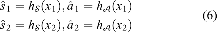
Our goal is to find two functions

They are estimated from the inference processes
As s and ai
in Eq. (4) are independent variables,
Adversarial disentangled feature learning
In this section, we present our feature disentanglement network in detail, including network architecture and the loss functions, which are summarized in Figure 2. At last, we introduce how to train the network and extend it to multiple domains.

Network architecture.
Network architecture
The motivation of the proposed network is to extract disentangled features from given images. To achieve it, we set to constrain features explicitly to fulfill the disentanglement requirement.
Firstly, our method uses an autoencoder as the feature extractor. Autoencoder is a widely used self-supervised machine learning method, where the encoder encodes the input as a feature and the decoder tries to reconstruct the original input from the feature. Our encoder is composed of two parts, namely the place encoder
Pure autoencoder is not enough for disentanglement, as there is no constraint for
where x
1 and x
2 are sampled from domains
Our autoencoder follows the widely used bottleneck architecture, where the input is downsampled into two smaller feature maps by the encoders, while the decoder tries to recover the input from those two feature maps. The discriminators take combinations of those feature maps as input and give one dimension as output (Figure 2). The detailed architectures of different experiments are listed in the appendix.
Autoencoder
To measure the reconstruction quality, different distances can be used. In the previous version, we used L2 loss for reconstruction, which can be expressed as follows 15

where xi
is an image sampled from some data distribution

where F is a pretrained VGG feature extractor. 58 With this perceptual loss, the reconstructed images are more semantically meaningful than the ones with L2 loss, which also leads to more meaningful features. This helps for boosting place recognition performance, as shown in the experiments.
Appearance compatibility discriminator
As pointed out in the last section, disentanglement requires that
During training,
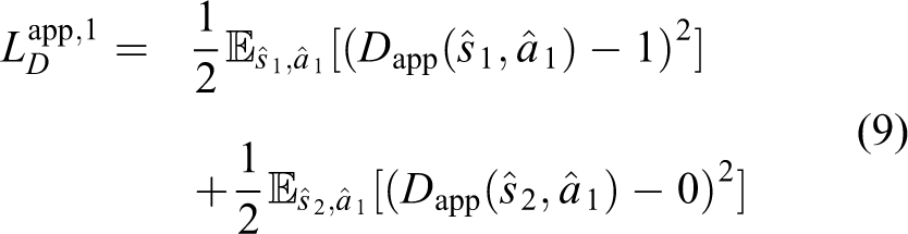
where
Encoders

It is worth noticing that
Equations (9) and (10) are formulated for the case that the first input image is sampled from
Place domain discriminator
With the appearance compatibility discriminator, we can only ensure that
Supervised methods like NetVLAD constrain features from the same place with different appearances to be the same,
10
which requires for alignment information. But as we hope to override the dependency on aligned data, we accomplish it in a different way. Constraining
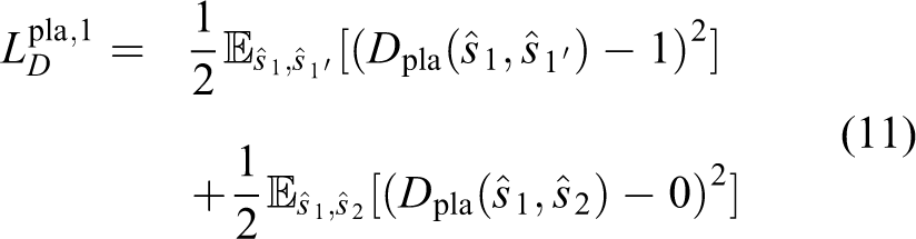
where

Similarly, we can have
Training strategies
The discriminators (


where
During training, the training datasets are augmented to increase robustness against viewpoint changes. For each image, we select four points on it randomly, and the surrounded area is cropped and wrapped into the original size. 11 Besides, the wrapped image is flipped horizontally randomly.
Extension: Multiple domain case
Based on this domain-unrelated architecture, we present how to extend our network to multiple domains. Assume that there are n domains, denoted by
This extension does not require additional parameters. To see it, one should note that the autoencoder is shared across different domains. Besides, the discriminators are also shared and domain-unrelated, which only use information between two domains. For example, if the inputs of
The extension enables that only one model is needed in a specific scene for long-term deployment. In the beginning, we have a baseline model trained from several domains. When new data with different appearances in the same area are available, the model can be fine-tuned by retraining on the dataset enhanced with newly collected data. The retraining does not require additional parameters. In contrast, style-transfer-based methods need new models to transfer new data into known styles. When new data come periodically, this will lead to quadratically increasing parameters. To see it, one can assume that there are m domains. To transfer each domain to others, they need to train
Experiments
We conduct several experiments to illustrate our method. Firstly, we validate the proposed network with two toy cases, including Linear Gaussian for quantitative analysis and Colored MNIST for qualitative analysis. Then, we apply our network to visual place recognition and demonstrate its performance in different perspectives, including basic performance, ablation study, and multiple-domain performance.
Toy case validation
Linear Gaussian
We test the network on a linear gaussian generative process with two domains to validate whether it can produce disentangled representation as desired. The reason to choose the linear model is that we can use correlation as a quantitative metric for disentanglement in the linear case. The generative process can be written as follows

where s and ai
are vectors with the dimension of ns
and na
, and they are sampled from two normal distributions, respectively, with
The encoders
To demonstrate the power of the two proposed adversarial losses, we compute the correlation matrix between the place feature
Figure 3(a) to (d) shows the case that

Correlation matrices for the linear toy case. Each subfigure is composed of two correlation matrices: correlation matrix between
Colored MNIST
The linear Gaussian is a simple toy case. To show the power of our method in a more complicated scenes, we propose
To investigate what has the network learned from this toy case, we visualize the place feature and appearance feature using t-distributed stochastic neighbor embedding (t-SNE).
66
As the dimensions of our features (1024 for
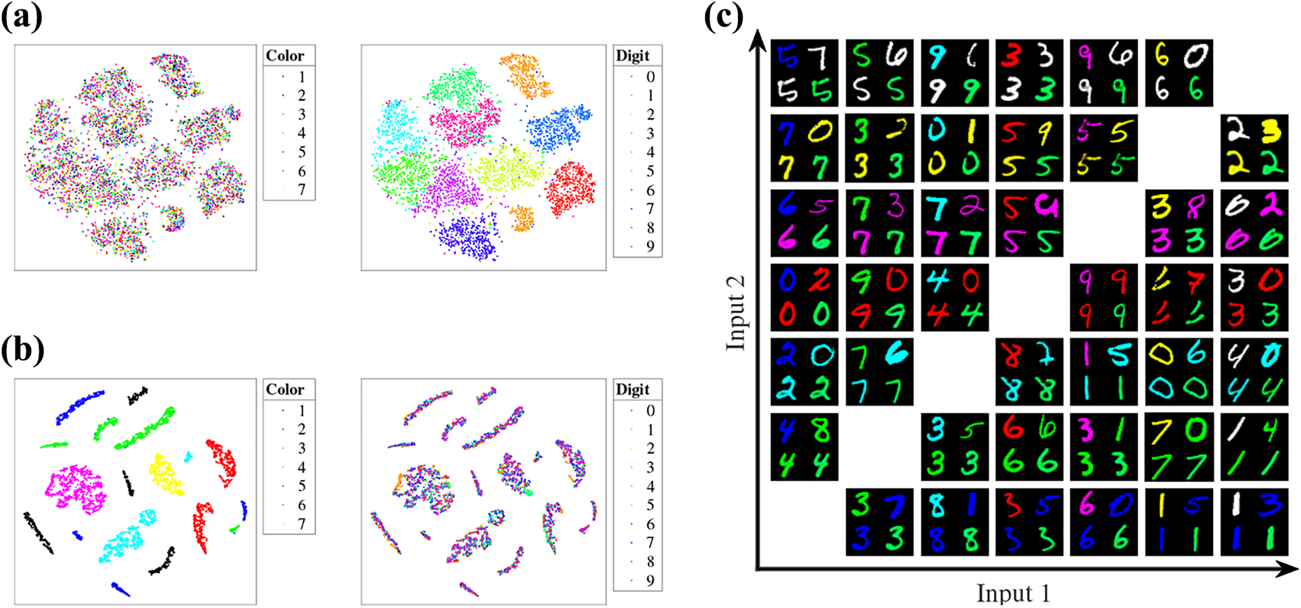
Visualization of the learned features on colored MNIST. Left: t-SNE visualization of place feature (Figure 4(a)) and appearance feature (Figure 4(b)) and right: image translation. (a)
We also try to analyze our network in image space. As done in some image-to-image translation literature,
67
we can replace the appearance features with those from another domain for the decoder to obtain image with different style. We implement this in two ways. Firstly, given two colored digits as inputs, we combine the place feature from the first digit and the appearance feature from the second digit and reconstruct a new digit through the decoder. The newly recovered digit is called translated image. Secondly, the appearance feature is replaced with a new vector filled with zeros, and the decoded image is called zero-appearance image. Results are presented in Figure 4(c). We sample images from every two domains. As there are seven domains in the dataset, there are
Datasets
To validate the proposed method on visual place recognition task, we test our network on three public datasets: Partitioned Nordland dataset, 32 Alderley Day/Night dataset, 7 and RobotCar-Seasons dataset. 68 Besides, we also experiment on a new dataset, YQ Day/Night dataset, which is collected in a campus environment with changing appearance and will be opened to the public (https://tangli.site/projects/academic/yq21).
Partitioned Nordland dataset
It is collected from a train on the same route (729 km) in four seasons (spring, summer, fall, and winter) with GPS data. In this article, four seasons are treated as four domains. The original Nordland dataset is used by many researches, 69,42 but they use different partitions for training and testing. This dataset proposes a reasonable partition of Nordland, where the whole route is partitioned into five segments, with two as training set and three as testing set. The training and testing sets have 24,570 and 3450 images for each domain, respectively. The GPS information is accurate enough to align between different domains. This dataset provides images without perspective changes and high-quality ground truth, thus it is useful for validating the ability to overcome appearance changes (Figure 5(a)).

Alderley Day/Night dataset
It is captured from a camera mounted on a car. It is constituted of two domains, one daytime and one nighttime, on an 8 km journey. As mentioned in their article, the GPS data are not reliable enough, thus the images are manually aligned frame by frame. 7 However, as the images are collected in an urban environment, the vehicle is moving with lateral and heading changes, which makes the alignment less reliable. Besides, the apparent differences between those two sessions are really large, making it challenging for place recognition. From Figure 5(b), one can see that sometimes it is even challenging for humans. Each domain in the dataset is split as a training and testing set with 10,007 and 4600 images, respectively. 32
RobotCar-Seasons dataset
It is based on the Oxford RobotCar dataset, which is recorded on a vehicle with six cameras under different conditions in the urban environment, with other sensors including INS, GPS, and LiDAR. 70 RobotCar-Seasons selects a subset of RobotCar dataset, with one reference traversal in overcast condition (overcast-reference) as database and nine traversals for query in different conditions. 68 The query set is further split as all-day and all-night, where all-day refers to images collected in the daytime, while all-night refers to images collected in the nighttime. In this article, only the all-night subset is used, as we want to validate our method in different domains. Thus, two domains, namely overcast-reference and all-night, are used for training and testing. The ground truth is obtained from large-scale structure from motion and initialized with INS data. One thing that should be mentioned is that the ground truth is only used in the testing phase, not in the training process. This dataset provides challenges in autonomous driving including appearance changes, perspective difference, and motion blur (Figure 5(c)).
YQ Day/Night dataset
It is a subset of the YQ dataset. 62 The original YQ dataset has 21 sessions, out of which we choose two for the place recognition task in this article. These two sessions become two domains in this dataset, namely day and night. The first session is collected in the morning, while the second one is collected in the evening (Table 1). The evening traversal is collected at the time when it is turning from day to night. Although this traversal only lasts for about 19 min, it contains a different appearance. Thus, it can be used to validate the robustness of algorithms against dynamic appearance changes in a short period. Sample images are shown in Figure 5(d). The ground truth is obtained from the LiDAR SLAM results. We split the trajectory into two folds, with the 60% beginning being the training set and the 30% ending as the testing set. The training set is sampled every 0.1 m, and the testing set is sampled every 2 m. As the data are recorded on a mobile robot controlled by a remoter at low speed, it can be seen as a representative in mobile logistics in a small area, with appearance and perspective changes.
Details of YQ Day/Night dataset.

Evaluation metrics and training details
We choose two widely used metrics for visual place recognition in the following experiments (except for RobotCar-Seasons which will be discussed later): area under curve (AUC) and accuracy (true positive rate). After the training is done, the place features are used as global descriptors for matching. The goal of visual place recognition is to find the nearest image to a given query image xQ
in database

Before computing the distances, all the features, including
Our network is trained with
Comparison methods
To illustrate the performance of our method on visual place recognition, several methods are selected as a comparison: Three methods based on handcrafted features (DBoW2, HOG, and DenseVLAD) are chosen as representatives of traditional methods.
24,27,55
For supervised methods, NetVLAD and method by Facil et al. are used to show their advantages and limitation.
10,32
As NetVLAD has opened the code for training NetVLAD, we also retrain NetVLAD on these datasets to see the improvement obtained from supervision. All settings follow the original article of NetVLAD, except that when training YQ Day/Night, the “nNegChoice,” “nTestSample,” and “nTestRankSample” are set as 20, 20, and 100, respectively, because the dataset is small. Besides, two style-transfer-based algorithms are also selected.
12,71
RobotCar-Seasons dataset uses different evaluation metrics. As described by the benchmark, RobotCar-Seasons dataset measures the performance using percentages of query images localized within three error tolerance thresholds. 68
Ablation study
Our method introduces two new adversarial losses to the autoencoder. To see whether the new losses work, we conduct an ablation study in this section. We selected the most challenging pair in Partitioned Nordland, namely winter and spring, as target domains. The experiment follows the same settings described in the last subsection, except the hyperparameters
Results are displayed in Table 2. We can see that the complete network (with
Ablation study.

AUC: area under curve.
Two domains
This section investigates the performances of different methods in the scenario with two domains. For Partitioned Nordland dataset, only the winter and spring sessions are chosen as two domains.
Experimental results are listed in Tables 3 and 4. Table 3 presents the performance of different methods on three of the mentioned datasets: Partitioned Nordland, Alderley Day/Night, and YQ Day/Night. To evaluate our method on RobotCar-Seasons dataset, we submit our results to the Visual Localization Benchmark (https://www.visuallocalization.net/benchmark). In Table 4, we also consider several methods on that benchmark as a comparison (only published place recognition algorithms are selected).
Performance of different methods.
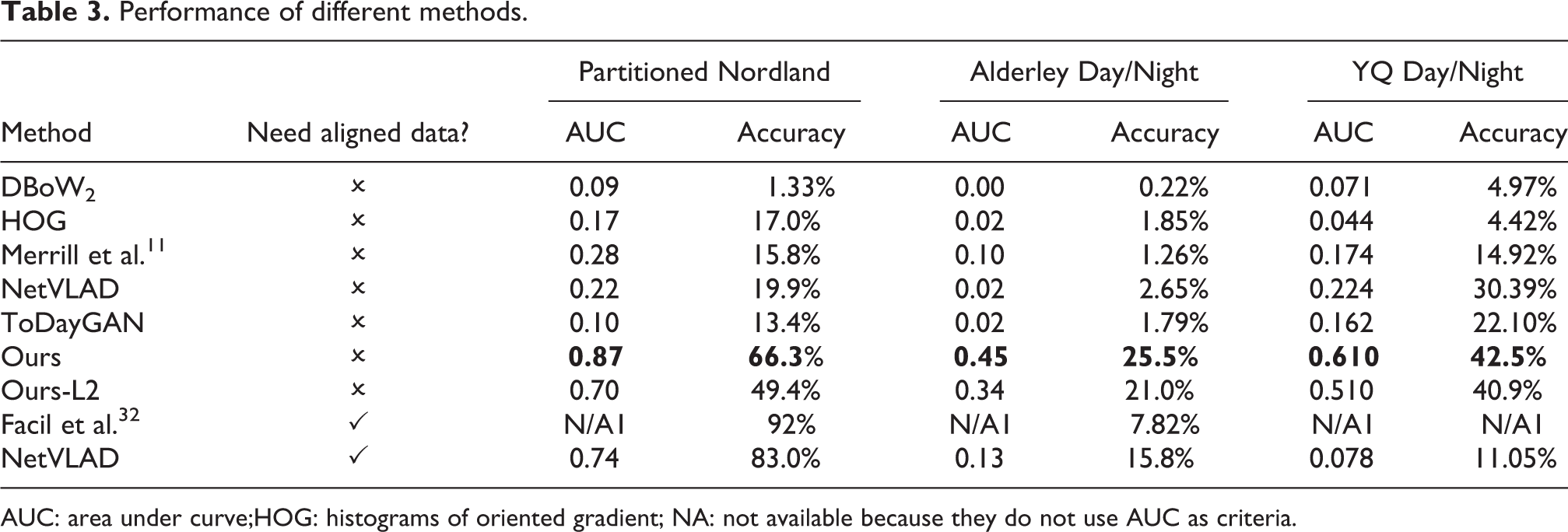
AUC: area under curve;HOG: histograms of oriented gradient; NA: not available because they do not use AUC as criteria.
Performance on RobotCar-Seasons.

Red: best performance; blue: second-best performance.
From Table 3, we can see that methods based on handcrafted features are not good at place recognition tasks with extreme appearance changes. For learning-based, the supervised methods outperform self-supervised ones in some dataset (Partitioned Nordland) as expected. However, our method is better than those supervised methods on some datasets (Alderley Day/Night and YQ Day/Night). There are two possible reasons. One is that supervised methods depend on the quality of alignment. As we described before, the alignment of Alderley Day/Night is not good enough somewhere, which may degrade the performance for supervised methods. Another reason is that the training set and testing set of YQ Day/Night have subtle differences as described above, which request for generalization ability for algorithms. Generally speaking, self-supervised methods outperform supervised methods in the sense of generalization.
Compared with other self-supervised methods, our method achieves comparable results. It shows the best performance on Partitioned Nordland, Alderley Day/Night, and YQ Day/Night. Combine with Table 4, we can find that our method and ToDayGAN perform better than other self-supervised methods on different datasets. One main difference between our method and ToDayGAN is that in our method the adversarial learning is applied directly to features, while ToDayGAN is on images. The transferred image by ToDayGAN looks realistic, but sometimes it still looks different from the original style image (the reader can see transferred images in the appendix). The reason is that in style transfer the same input image can generate different output. Especially, Partitioned Nordland has a slight appearance difference in the same domain, resulting in the miss-matching problem. Conversely, the appearance of the same domain in RobotCar-Seasons is quite stable, that is why ToDayGAN outperforms our method on RobotCar-Seasons in some criteria.
To see the improvement brought by perceptual loss, we also trained our network with L2 reconstruction loss (Our-L2 in Table 3). From Table 3, we can see that perceptual loss has an obvious increase compared to L2 loss. This finding illustrates that the learned features can improved by reconstructing high-level features instead of reconstructing original images.
We also try to explore what does the network learns by generating images from cross-domain features. For specific, we feed place features from one domain (Figure 6(a)) with appearance features from the other domain (Figure 6(b)) into our network to see what will be generated from the decoder G (Figure 6(c)). In Figure 6(c), one can find that the place information (e.g. tracks, buildings, and traffic lights) is determined by images in the first row (Figure 6(a)), while the appearance information (e.g. color of the ground, illumination) is determined by the second row (Figure 6(b)). This result satisfies our motivation: the place information is embedded in the place feature, while the appearance feature controls the appearance of the reconstructed images. To further illustrate what is learned in the place feature, we replace all the appearance features with all-zero vectors (Figure 6(d)). All the zero-appearance images look to have a similar appearance, while their place information remains the same as the first row (Figure 6(a)). These two findings demonstrate that the proposed method can disentangle the input image across appearance changes.

Translated and zero-appearance images of Partitioned Nordland dataset. Each image in (c) is generated from the place feature of an image from (a) in the same column and appearance feature of an image from (b) in the same column, while an image in (d) is generated from place feature of (a) and an all-zero appearance feature. Columns 1 to 5:
Multiple domains
One novelty of our network is that it is designed to be trainable with multiple domains without additional parameters. The benefit is that when new data from different domain come, we can retrain our network without increasing model capacity. We use Partitioned Nordland dataset to illustrate this point as it has four domains. Firstly, for every two domains, we train a network and evaluate it on the testing set. In this process, we have 12 models in total. Secondly, we train a unified model with four domains as the training set and then evaluate it on every two domains. In this stage, only one model is obtained.
Table 5 is the comparison results between two-domain models and multiple-domain models. We can see that by fusing more domains, our network achieves comparable performance to the two-domain models. However, the two-domain network needs 12 models, while the multiple-domain network needs only 1 model. It means our method can be extended to more domains while keeping the same model complexity. This is very useful when deploying deep learning networks in an environment with changing appearance.
Performance comparison between two-domain and multiple-domain models.a

AUC: area under curve.
a Each item corresponds to two-domain/multiple-domain.
Conclusion
We propose a feature disentanglement network for place recognition, which is composed of an autoencoder and two discriminators. By training the network in an adversarial manner, we can obtain domain-unrelated and domain-related features from multiple-domain data. The appearance compatibility discriminator enforces the appearance feature to be invariant to place content, while the place domain discriminator constrains the place feature to be robust against appearance changes. Qualitative and quantitative results on two two-domain cases demonstrate that our network is capable to obtain disentangled representation. Experiments on four datasets show that our method achieves favorable performance in visual place recognition tasks. Additionally, our network can be extended to multiple domains without increasing model capacity and sacrificing performance. We also open a new place recognition dataset for the research community.
Appendices
Network architecture
Networks for the linear case, colored MNIST, and place recognition are listed in Tables 6
to 8, respectively. Conv-(Nn, Kk, Pp, Ss) denotes a convolution with output channels of n, kernel size of
Network for linear case.

LReLU: leaky rectified linear unit.
Network for colored MNIST.

ReLU: rectified linear unit.
Network for place recognition.

ReLU: rectified linear unit; IN: instance normalization; LN: layer normalization.
Samples of style transfer
Figure 7 is the sample output by Anoosheh et al. 12 , including three datasets (Partitioned Nordland, Alderley Day/Night, and YQ Day/Night).
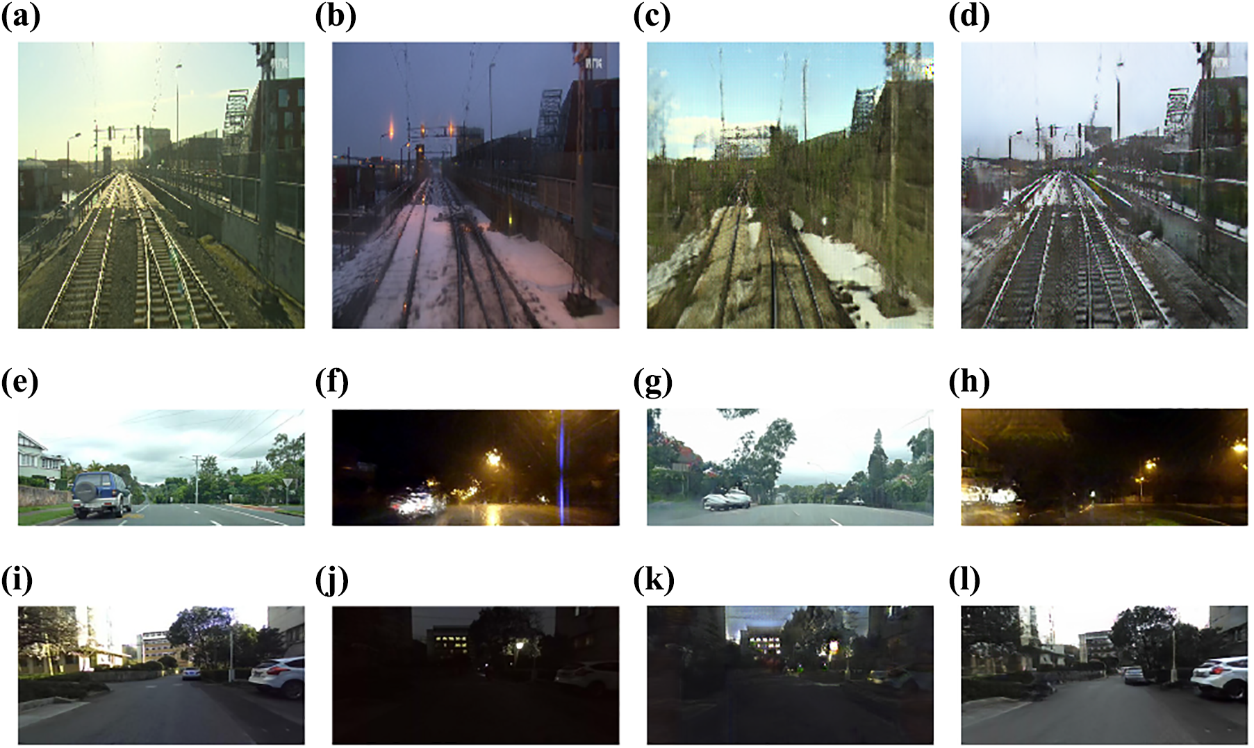
Image style transfer results of ToDayGAN. 12 Row 1: Partitioned Nordland dataset; row 2: Alderley Day/Night dataset; and row 3: YQ Day/Night dataset. (a) Spring; (b) winter; (c) winter to spring; (d) spring to winter; (e) day; (f) night; (g) night to day; (h) day to night; (i) day; (j) night; (k) night to day; and (l) day to night.
Footnotes
Declaration of conflicting interests
The author(s) declared no potential conflicts of interest with respect to the research, authorship, and/or publication of this article.
Funding
The author(s) disclosed the receipt of the following financial support for the research, authorship, and/or publication of this article: This work was supported in part by the National Nature Science Foundation of China under Grant 61903332, and in part by the Natural Science Foundation of Zhejiang Province under grant number LGG21F030012.