Sage Journals: Discover world-class research

Abstract

Innovative applications in rapidly evolving domains such as robotic navigation and autonomous (driverless) vehicles rely on motion planning systems that meet the shortest path and obstacle avoidance requirements. This article proposes a novel path planning algorithm based on jump point search and Bezier curves. The proposed algorithm consists of two main steps. In the front end, the improved heuristic function based on distance and direction is used to reduce the cost, and the redundant turning points are trimmed. In the back end, a novel trajectory generation method based on Bezier curves and a straight line is proposed. Our experimental results indicate that the proposed algorithm provides a complete motion planning solution from the front end to the back end, which can realize an optimal trajectory from the initial point to the target point used for robot navigation.

Keywords

Motion planning pathfinding trajectory generation jump point search Bezier curves

Introduction

Simultaneous localization and mapping (SLAM) and motion planning are two of the most critical problems of mobile robots. After solving the SLAM problem, using task instructions and known map information to realize robot navigation is the key and difficult point of autonomous mobile robot research. Motion planning (also known as the navigation problem or the piano mover’s problem¹) is a term used in robotics for the process of breaking down the desired movement task into discrete motions that satisfy movement constraints and possibly optimize some aspect of the movement.²

The old-school pipeline planning algorithm can be divided into front-end path planning and back-end trajectory generation. Path planning mainly refers to global path planning based on the given map, planning a path from the initial to the robot’s target. Generally speaking, only the workspace’s geometric constraints are considered in the path planning process, not the robot’s kinematic and dynamic constraints (there are also some path planning methods based on kinodynamic). The path information only contains the route from the initial to the target. It does not consider the robot’s kinematic model, so the robot control instructions cannot be generated directly.

The common path planning algorithms can be divided into graph search-based path planning algorithm, sampling-based path planning algorithm, and neural network-based path planning algorithm. The sampling-based path planning algorithm scatters points in space according to a certain strategy and then starts from an initial tree and uses edge lines to expand the tree until it triggers the termination condition (reaching the target point or near the target point). However, its random sampling characteristics lead to slow search speed and an unsmooth path. Moreover, this algorithm has poor adaptability in an unstructured, complex environment.

The graph search method is the most intuitive method of path planning. It first constructs the connection graph in free space and then searches on the connection graph until the target point is found. The A* algorithm is a widely used graph search method in robot path planning. It adds a heuristic function h(n) to the Dijkstra algorithm, representing the minimum estimated cost from the current node to the target point. In the literature,³ an improved strategy of the A* algorithm is proposed to simplify the path and to calculate the robot’s rotation direction and the angle at the inflection point. Jump point search (JPS) algorithm proposed by Harabor and Grastien⁴ retains the framework of A* algorithm and further optimizes the operation of the A* algorithm to find the successor nodes. The algorithm expands the nodes according to the current node’s direction and based on the JPS strategy, significantly reducing the search space. Dolkov et al.⁵ proposed a hybrid A* path search algorithm to meet the vehicle kinematic characteristics. It can plan the feasible path close to the global optimal but cannot ensure that the vehicle’s curvature at the initial and the target position changes continuously. In the literature,^6,7 A* search results and Reeds–Shepp curve were used as a heuristic function, and the Reeds–Shepp curve was used to expand nodes, which accelerated the search speed.

Trajectory planning is also important for mobile robots. It can be further divided into model predictive control and geometric trajectory-based planning methods. The common trajectories include spiral curve,⁸ β spline curve,⁹ Bezier curve,^10,11 η curve,¹² and so on. Chen et al.¹³ proposed to use the Bezier curve for trajectory planning of wheeled robots, and Jolly et al.¹¹ studied the trajectory planning based on the third-order Bezier curve. The proposed method only considered the acceleration constraint, not the curvature constraint. However, Choi et al.¹⁴ planned the continuous curvature trajectory based on the Bezier curve, which connected the lower-order Bezier curves to generate a continuous curvature trajectory.

Here, an improved method of mobile robot motion planning is proposed. In front-end path planning, an improved JPS algorithm is proposed, optimizing the heuristic function and simplifying the turning point. Unlike the traditional JPS algorithm, the proposed algorithm first considers the distance and direction as the heuristic function. It then trims the redundant extension nodes to improve path planning efficiency. An improved trajectory optimization algorithm based on a straight line and Bezier curve is proposed in the back-end trajectory planning. In this algorithm, the Bezier curve is used to generate the trajectory at the path’s turning point. The straight line segment is used to retain the path at the nonturning point to generate a trajectory with continuous size, direction, and curvature.

The remainder of this article is organized as follows. The second section proposes the algorithmic foundations used in the front end and describes the heuristic function and postprocessing. The third section introduces the trajectory planning algorithm, which is based on straight lines and the Bezier curve. A simulation evaluation is carried out to demonstrate the proposed framework’s effectiveness in the fourth section, followed by conclusions in the fifth section.

Front-end path finding: An improved jump point search algorithm

Definition of jump point search

A* algorithm is a typical heuristic search algorithm,^11,12 as shown in the following formula

f (n) = h (n) + g (n)

where f(n) is the evaluation function of node n, g(n) is the actual cost from the initial node to N node in the state space, and h(n) is the estimated cost of the optimal path from N node to the target node.

A* algorithm takes all neighbor nodes into account when expanding nodes. Therefore, the number of points in the stack will be large while the search efficiency became slow. JPS algorithm eliminates many uninterested points by looking for jump points, which improves the algorithm’s speed. Similar to A* algorithm, the JPS algorithm also uses f(n) = h(n) + g(n) expansion nodes to achieve planning, in which the heuristic function h(n) largely determines the efficiency of the algorithm. The common heuristic functions usually use Manhattan distance or Euclidean distance. Although the estimated h(n) of these two distances is less than the actual cost h(n)* (where Manhattan distance is only applicable to the grid connected by lines), there are two problems for both A* and JPS:

h(n) is not tight enough, and h(n) is far less than h(n)*, which lead to more nodes and low efficiency;

Only the distance information is considered, but the direction information is not taken into account, which leads to the difficulty of trajectory optimization in the later stage.

Proposed algorithm

A new h(n) heuristic function is proposed to solve these two previously mentioned problems, as shown in equation (2)

h (n) = a L - b cos α

where a and b are the weights of distance and direction, L is the distance information, as shown in equation (3), and cosα is the direction information that represents the angle between the parent node and the expanded node and the angle between the expanded node and the target point, which represents the cost of direction needed to expand according to this node.

When the two directions are the same, the value of cosα is +1 and the direction cost is the minimum, but when the two directions are opposite, the direction cost of −1 is the maximum

L = d x + d y - (2 - \sqrt{2}) \times min (d x, d y)

where dx and dy represent the distances from the current node A to the target point B on the x-axis and y-axis, respectively.

As shown in Figure 1, the green and blue lines represent the Euclidean distance and Manhattan distance of the two points on the grid, respectively, while the red line represents the real shortest distance of the grid under the eight connections.^15
–17 Among them, Euclidean distance refers to the straight line distance in Euclidean space, and his formula in two-dimensional (2D) space is

L = d x + d y

Manhattan distance refers to the sum of absolute axes of two points in the standard coordinate system.

Figure 1.

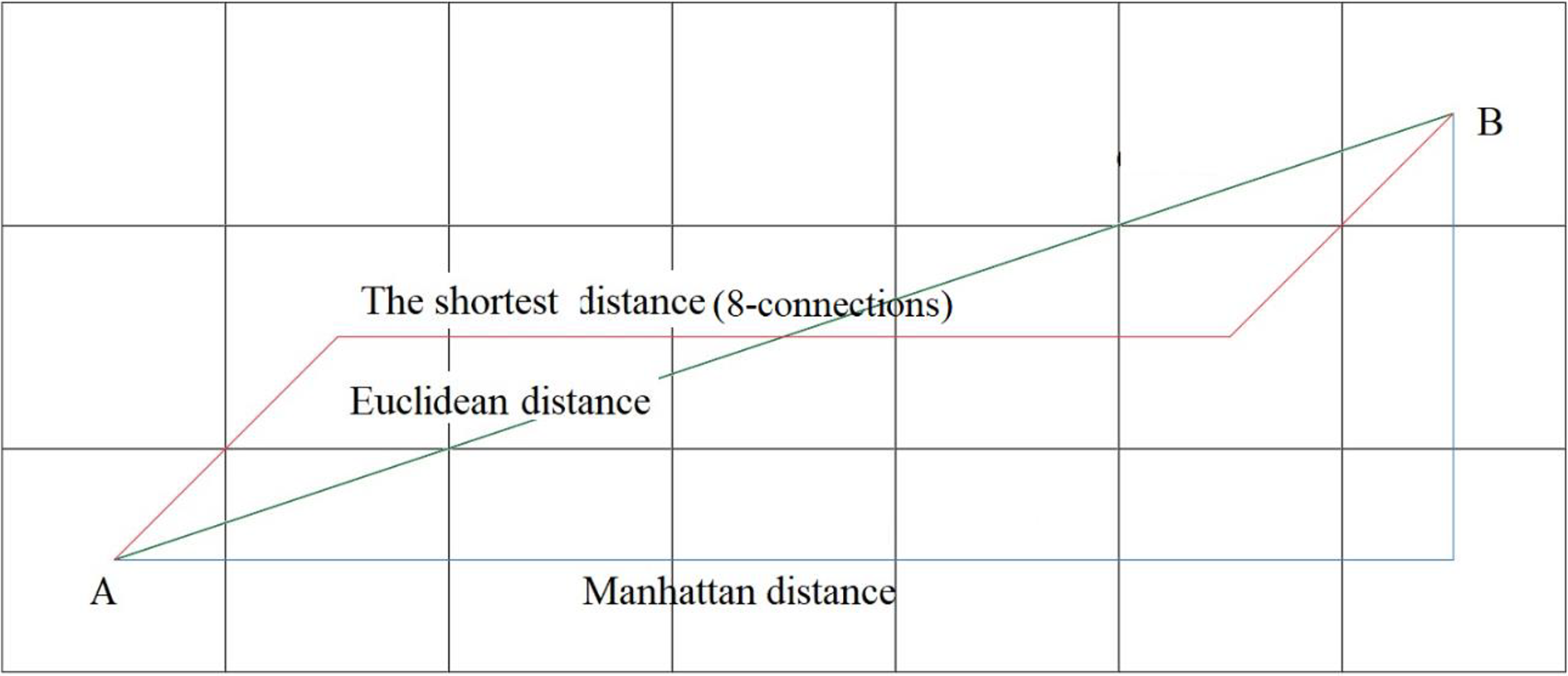
Heuristic function. Green line: Euclidean distance; blue line: Manhattan distance; red line: shortest distance of the grid under the eight connections.

This improved JPS algorithm can get the planning path more efficiently and accurately. Although the JPS algorithm can significantly reduce the number of extended nodes, it will expand the nodes in the area with obstacles, which will increase the difficulty of trajectory optimization in the later stage. Based on the above description, the turning point is trimmed to improve the path’s smoothness further. For all extended nodes (P ₀; P ₁,…, P_N ), if the slopes of the lines P_n ₋₁ P_n and P_nP_n ₊₁ formed by adjacent nodes are different, then connect P_n ₋₁ and P_n ₊₁. If P_n ₋₁ P_n ₊₁ does not pass through the obstacles, the original P_n ₋₁ P_n and P_nP_n ₊₁ are discarded, and P_n ₋₁ P_n ₊₁ is retained. Then, the path is simplified by comparing P_n ₋₁ P_n ₊₁ and P_n ₊₁ P_n ₊₂, and so on.

As shown in Figure 2, the blue line segment is the JPS algorithm’s path, and five planning points are obtained. Using the JPS algorithm, the path is simplified, and the red line segment results from simplification. The algorithm connects points P ₀ and P ₂, because line P ₀ P ₂ does not pass through the obstacles, so the original P ₀ P ₁ and P ₁ P ₂ are discarded, and P ₀ P ₂ is retained. It continues to connect points P ₀ and P ₃, line P ₀ P ₃ passes through the obstacles, so it abandons line P ₀ P ₃ and keeps line P ₀ P ₂. Starting from point P ₂ again, it connects P ₂ P ₄, P ₂ P ₄, and so on. Finally, P ₂ P ₃, P ₃ P ₄, P ₄ P _5, and P ₅ P_N are discarded, and P ₂ P_N is retained. It can be seen from Figure 2 that the expanded nodes P ₁, P ₃ , P ₄, and P ₅ are discarded, and only the node P ₂ is retained. Although the expanded nodes of the algorithm remain unchanged, the improved planning path is more efficient.

Figure 2.

Deleting redundant points based on JPS algorithm; blue lines: JPS algorithm; red line: simplified by the improved algorithm. JPS: jump point search.

The whole improved path planning algorithm based on JPS is shown in Algorithm 1.¹⁸

Algorithm 1

Improved JPS

Back-end trajectory generation based on Bezier curve and straight line segment

Trajectory generation

The proposed path planning algorithm can generate an optimal path, but it does not consider the robot’s kinematic model. The resulting path is not smooth, and the curvature is noncontinuous. Therefore, based on the path planning algorithm mentioned above, the Bezier curve is used to optimize the trajectory, which improves the smoothness of the global path.

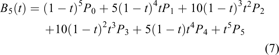
In 1962, Pierre Bézier, a French mathematician, studied a drawing curve method by vectors and gave a detailed formula called the Bezier curve. Bezier curve defines the starting point, endpoint, and control points of the curve. By adjusting the control points, the shape of the curve can be changed. The general form of the Bezier curve is shown in equation (5)

B_{j} (t) = P_{0} b_{n}^{0} (t) + P_{1} b_{n}^{1} (t) + \dots + P_{n} b_{n}^{n} (t) = \sum_{i = 0}^{n} P_{i} b_{n}^{i} (t)

where

b_{n}^{i} (t) = (\begin{matrix} n \\ i \end{matrix}) t^{i} {(1 - t)}^{n - i}

The characteristics of the Bezier curve are as follows:

Endpoint interpolation: Bezier curve always starts from the first control point and ends at the last control point. It does not pass through any other control points;

Convex hull: Bezier curve is in convex hull defined by all these control points;

Differential: The derivative curve B′(t) of (t) is also a Bezier curve, and its control point is defined by $n \cdot (c_{i + 1} - c_{i})$ , where n is the order;

Fixed time interval: Bezier curve is always defined in the range of [0,1].

The improved JPS algorithm plans a line segment from the initial point to the target point. A curve segment with the continuous position,¹⁹ direction, and curvature can be further planned using the quartic Bezier curve, realizing the trajectory generation of robot navigation, as shown in green in Figure 3. This is based on the assumption that the direction of both the initial and the target points is horizontal to the right. We propose a trajectory generation algorithm based on the mixture of Bezier curve and straight line, which ensures the continuity of direction, position, and curvature. Unlike the traditional Bezier curve trajectory optimization, the Bezier curve and straight line segment trajectory require that each segment of the Bezier curve and line segment should also have a continuous position, direction, and curvature. The expression of the quintic Bezier curve is shown in equation (7). The curve itself needs six control points, and there are four intermediate control points besides the starting point and the endpoint. For the proposed algorithm, if the path has N turning points, the whole path has N + 2 path points: P ₀ (initial point) P ₁, P ₂,…, P _N and P_N ₊₁ (target point), N + 1 break line. Accordingly, N Bezier curves and N + 1 straight line segments after trajectory optimization using quintic Bezier curve straight line segment, and their positions, directions, and curvature are continuous

B_{5} (t) = {(1 - t)}^{5} P_{0} + 5 {(1 - t)}^{4} t P_{1} + 10 {(1 - t)}^{3} t^{2} P_{2} + 10 {(1 - t)}^{2} t^{3} P_{3} + 5 (1 - t) t^{4} P_{4} + t^{5} P_{5}

Figure 3.

Trajectory generation by Bezier curve based on Figure 2, green curve.

Because the algorithm requires the Bezier curve’s curvature and the straight line segment to be continuous, the curvature at the junction of the Bezier curve and straight line segment is 0. According to the control points property of the Bezier curve, control points $P_{i 1}, P_{i 2}, and P_{i 3}$ are collinear, and $P_{i 4}, P_{i 5}, and P_{i 6}$ are collinear. In addition, since the position of the Bezier curve and straight line segment is continuous, these six control points must be on the original straight line segment, as shown in Figure 4. Considering the convexity of the Bezier curve, the trajectory will be inside the line segment. Furthermore, the trajectory must be shorter than the planning path.^20
–22

Figure 4.

Control points of Bezier curve, $P_{i - 1}, P_{i}, P_{i + 1}$ are the points after path planning, $P_{i 1}, P_{i 2}, P_{i 3}, P_{i 4}, P_{i 5}, P_{i 6}$ are the control points of the Bezier curve.

The most important part to replace the original straight line segment with Bezier curve is mainly divided into two steps

1. Control points calculation of the Bezier curve.

As shown in Figure 3, to generate the Bezier curve, six control points $P_{i 1}, P_{i 2}, \dots, and P_{i 6}$ form the quintic, where the Bezier curve is determined. Then, the angle is set between $P_{i - 1} P_{i}$ , $P_{i} P_{i + 1}$ , and the positive direction of the x-axis is $α, β$ , and the distance between the six control points and the inflection point P_i is $d_{1}, d_{2}, \dots, d_{6}$ . Then, the coordinates of the six control points could be computed using equation (8) as follows

\{\begin{cases} P_{i 1, x} = P_{i, x} - d_{1} cos α \\ P_{i 1, y} = P_{i, y} - d_{1} sin α \\ P_{i 2, x} = P_{i, x} - d_{2} cos α \\ P_{i 2, y} = P_{i, y} - d_{2} sin α \\ P_{i 3, x} = P_{i, x} - d_{3} cos α \\ P_{i 3, y} = P_{i, y} - d_{3} sin α \\ P_{i 4, x} = P_{i, x} + d_{4} cos α \\ P_{i 4, y} = P_{i, y} + d_{4} sin α \\ P_{i 5, x} = P_{i, x} + d_{5} cos α \\ P_{i 5, y} = P_{i, y} + d_{5} sin α \\ P_{i 6, x} = P_{i, x} + d_{6} cos α \\ P_{i 6, y} = P_{i, y} + d_{6} sin α \end{cases}

2. Optimal generation of the Bezier curve

By parameterizing the control points of the Bezier curve, the trajectory determined by d ₁, d ₂,…, and d ₆ satisfies the kinematic constraints. For the trajectory, the shorter the path and the smaller the curvature change, and the less the cost. In this article, the path length and curvature change of the Bezier curve are used as optimization functions. Then, the trajectory optimization problem can be represented as a constrained nonlinear optimization problem^23
–25

\begin{array}{c} minimize : (\int_{0}^{1} \sqrt{{P^{'}}_{x} {(u)}^{2} + {P^{'}}_{y} {(u)}^{2}}) + (c_{max} (u) - c_{min} (u)) \\ s
.t
. c_{max} (u) \leq c_{max} \\ 0 < d_{3} \leq d_{2} \leq d_{1} \\ 0 < d_{4} \leq d_{5} \leq d_{6} \\ e (u) > e_{min} \end{array}

As shown in equation (9), the nonlinear optimization includes two terms: the first term is the Bezier curve’s length. The second term is the maximum and minimum curvature interpolation, representing the range of curvature variation. The constraints can be divided into three categories: the first type constrains the curvature boundary; the second type constrains the location of control points; the third category constrains the obstacles.

Because of the Bezier curve’s convex hull property, if the convex polygon formed by control points does not intersect with the obstacle, the Bezier curve will not intersect with the obstacle outside the convex polygon. Since all of the control points are on the line segment of the original planning, if the line segment $P_{i 1} P_{i 6}$ does not intersect the obstacle, the obstacle constraint is satisfied. Let $e (u)$ be the distance between the line segment $P_{i 1} P_{i 6}$ and the obstacle, it should be bigger than a certain safety threshold.

Suppose the direction of the initial point or the target point of the whole path is different from the direction of the corresponding straight line segment, in that case, it is required to move in the same direction as the straight line according to the maximum turning capacity.

Speed planning

Through path planning and trajectory generation, a trajectory satisfying the kinematic constraints can be obtained. To ensure that the mobile robot can move according to the trajectory, the trajectory’s speed planning is still needed.

Figure 5 shows the front wheel steering mobile robot’s kinematics model, where the curvature is generated using equation (10)

κ = \frac{1}{r} = \frac{tan α}{L} .

The kinematic model of the mobile robot is generated using equation (11)

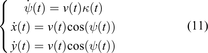
\{\begin{matrix} \dot{ψ} (t) = v (t) κ (t) \\ \dot{x} (t) = v (t) cos (ψ (t)) \\ \dot{y} (t) = v (t) cos (ψ (t)) \end{matrix}

Figure 5.

The model of mobile robot.

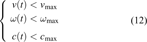
When the mobile robot moves, the following constraints should be considered: (1) The maximum velocity constraint, (2) maximum acceleration constraint, (3) maximum curvature constraint, (4) velocity continuity constraint, (5) acceleration continuity constraint, and (6) curvature continuity constraint. Because this article uses the Bezier curve and straight line segment as the trajectory generation algorithm, the system meets the speed continuous constraint, continuous acceleration constraint, and curvature continuous constraint.

The speed and curvature constraint of the robot is defined by equation (12)

\{\begin{matrix} v (t) < v_{max} \\ \begin{matrix} ω (t) < ω_{max} \\ c (t) < c_{max} \end{matrix} \end{matrix}

Firstly, the speed constraint is applied to each planning point, and then, the iteration started from the initial speed, as shown in equation (13)

a (t) < a_{max}

The acceleration of the robot consists of radial acceleration and tangential acceleration, as stated in equation (14)

\frac{a_{t}^{2}}{a_{t max}^{2}} + \frac{a_{r}^{2}}{a_{r max}^{2}} = 1

Using the maximum acceleration to calculate the velocity value of the next planning point, then $v_{k + 1}$ can be determined using equation (15)

v_{k + 1} < v_{k} + a_{t} Δ

The relationship between velocity and trajectory length is computed using equation (16)

v_{k + 1}^{2} - v_{k}^{2} = 2 a_{t} Δ s (t)

where $Δ s (t)$ is the trajectory length between two planning points.

In this method, each planning point’s velocity can be calculated iteratively, and the acceleration constraint is satisfied.

Simulation and experiments

To the path planning and trajectory generation algorithm proposed in this article, the algorithm is simulated by MATLAB, and an experiment is carried out for a wheeled mobile robot.²⁶

Simulation environment

To examine the proposed algorithm’s effectiveness in this article, MATLAB is selected as the simulation tool. As shown in Figure 6, the green dot is the static obstacle, the blue * is the initial point, and the red * is the target point. As can be seen, the environment has the characteristics of multiple static obstacles. In this 2D static global environment, the traditional algorithm and the algorithm proposed in this article are compared and simulated.

Figure 6.

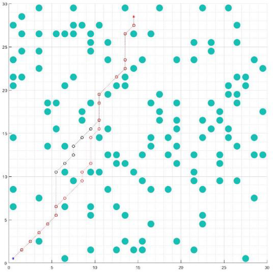
Simulation result of improved heuristic function. The green dot is the static obstacle, the blue * is the initial point, and the red * is the target point. The traditional JPS searches red broken line segment and black line segment is searched by improved heuristic function JPS. JPS: jump point search.

Improved jump point search simulation results (improved heuristic function)

The comparative simulation of global planning is carried out in a 2D static environment, as shown in Figure 6. The red broken line segment is the path searched by the traditional JPS algorithm. JPS algorithm can complete the path search from the initial point to the target point. However, it can be seen that the global path is close to the obstacles, and it has a large number of turns. This is because the traditional heuristic function only considers the Euclidean distance and does not consider the direction factor. It will increase the robot’s motion cost and increase the back-end trajectory optimization difficulty in practical application.

The improved heuristic function is used to carry out simulation experiments, as shown in Figure 6. The black broken line segment is the path searched using the improved heuristic function. Due to the direction factor’s consideration, the algorithm has been moving toward the target direction, reducing the number of turns and keeping the distance cost not to grow.

Improved jump point search simulation results (trimming the turning point)

Compared to A* algorithm, the JPS algorithm dramatically reduces the number of expansion points, but because the node expansion process uses eight connected search neighborhoods, the expansion can only move along the orthogonal and diagonal direction. Besides, the JPS algorithm expansion relies on force neighbor, it produces many expansion points on the same line. These shortcomings will increase the cost of the algorithm and the difficulty of the back-end trajectory optimization. Using the turning point trimming method makes up for the shortcomings of the traditional JPS algorithm.

As shown in Figure 7, the blue dotted line is the original JPS planning path, and the blue point is the extension point; after the improved algorithm, the red point is the extension point after trimming, and the solid red line is the trimmed path. The algorithm further reduces the number of turning points and shortens the path length. Furthermore, as described in the back-end trajectory optimization in the third section, fewer planning points contribute to the optimization algorithm’s efficiency, and the curvature of the planning curve changes less. The comparison of the proposed and JPS algorithm is given in Table 1. The proposed algorithm can reduce the cost both in distance and direction, and the time cost increases with the node trimming.

Table 1.

Comparison of the cost results of the proposed and JPS algorithms.

Method	Cost of distance	Cost of direction	Number of points	Planning time (s)
JPS	42.53	8.635	24	2.251
Proposed	42.02	6.004	8	2.762

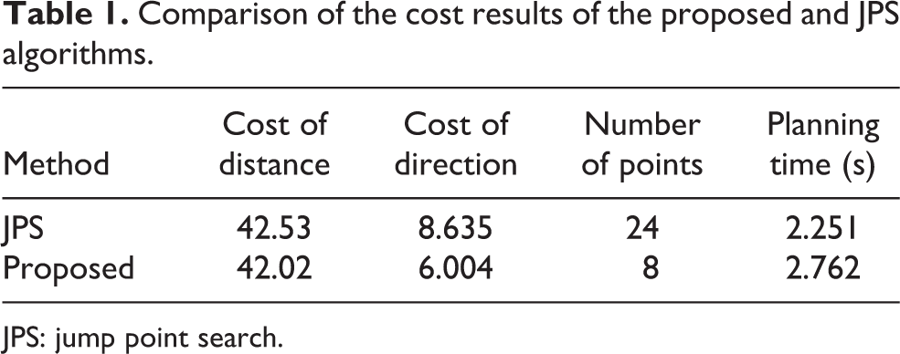
JPS: jump point search.

Figure 7.

Simulation result of trimming the turning point. The blue dotted line is the original JPS extension path, and the solid red line is the trimmed path. JPS: jump point search.

Improved trajectory generation simulation results

An optimized path can be obtained after the improved path planning algorithm based on the improved JPS algorithm. On this basis, the trajectory generation algorithm based on the Bezier curve and straight line segment proposed in the third section can further generate the trajectory from the initial point to the target point.

As shown in Figure 8, the blue dotted line segment results from the front-end path planning, and the red solid line segment is the optimized trajectory. It can be seen from the figure that the generated trajectory is smooth and continuous, which can avoid obstacles from the initial point to the target point and reduce the length of the original path.

Figure 8.

Simulation result of trajectory generation; the blue dotted line is the front-end path based on improved JPS, and the solid red line is the optimized trajectory. JPS: jump point search.

Figure 9 shows the curvature under the trajectory. It can be seen from the figure that the curvature value of the whole trajectory is continuous, which ensures the minimum curvature under the premise of obstacle avoidance.

Figure 9.

The curvature of the trajectory curvature.

Motion experiment of a wheeled robot

In this article, a wheeled robot is used to plan mobile robot navigation in the indoor environment. The maximum curvature of the robot is 1 m⁻¹, the maximum linear velocity is 0.52 m s⁻¹, the maximum tangential acceleration is 0.2 m s⁻², and the maximum radial acceleration is 0.4 m s⁻².

The experimental environment is an indoor laboratory environment, using an RGB-D camera as a robot vision sensor. The camera’s point cloud map in the ROS environment is used as the environment map input. Firstly, the point cloud map is transformed into a three-dimensional (3D) grid map based on octree, and then, it is transformed into a 2D grid considering the height threshold. On this basis, the size of the mobile robot is considered for size expansion. Figure 10(a) shows a point cloud map of the original scene, Figure 10(b) shows a 3D grid map based on octree, and Figure 10(c) depicts the 2D grid map considering the overall experimental environment after the expansion of the size of the mobile robot.

Figure 10.

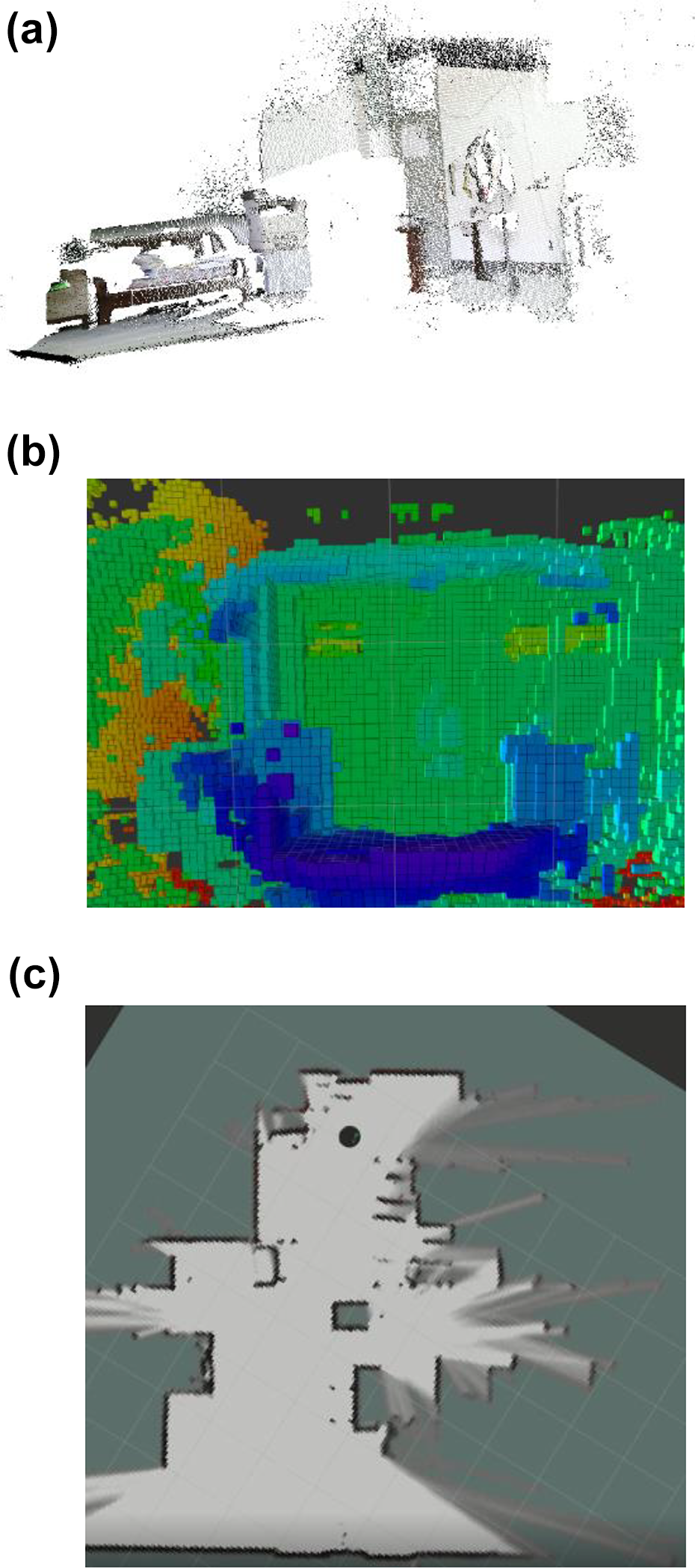
Grid map of indoor scene. (a) a point cloud map of the original scene, (b) 3D grid map, and (c) 2D grid map.

Figure 11 is a robot motion planning according to the algorithm proposed in this article in the ROS environment, while Figure 12 is the speed planning according to this path. The wheeled robot accelerates to move along the planned path from rest, completes the whole path, and stops at the end. It can be seen from the experiment that the speed planning algorithm proposed in this article ensures the continuity and boundedness of velocity and acceleration.

Figure 11.

Trajectory of wheeled robot.

Figure 12.

Velocity changes in trajectory of wheeled robot.

It can be seen from Figure 11 that based on the known environment map, the robot uses its own camera to collect the real-time map of the surrounding environment and modify the real-time grid map around the robot to meet the requirements of real-time obstacle avoidance for dynamic obstacles.

Conclusions

An improved JPS and Bezier curve algorithm has been introduced in motion planning. Firstly, the heuristic function based on distance and direction is used to describe the estimated cost more accurately from the current point to the target point. Secondly, the redundant turning points are trimmed to reduce the cost and provide a better trajectory generation premise. A novel trajectory generation method based on the Bezier curve and a straight line is proposed in the back end, which provides a trajectory generation algorithm with continuous size, direction, and curvature.

The simulation results show that the algorithm does the following:

It realizes the optimal path planning from the beginning to the end;

The position, direction, and curvature of the track are continuous;

The track length and time cost have good performance.

Therefore, the algorithm provides a complete scheme for the motion planning and navigation of mobile robots. Besides, through the indoor environment robot’s planning experiments, the mobile robot can get real-time information of the environment through the RGB-D camera and achieve real-time obstacle avoidance during the global path and trajectory planning.

The results demonstrate that the proposed algorithm has provided an optimal path and trajectory, which can be used for robot navigation.

Footnotes

Declaration of conflicting interests

The author(s) declared no potential conflicts of interest with respect to the research, authorship, and/or publication of this article.

Funding

The author(s) disclosed the receipt of the following financial support for the research, authorship, and/or publication of this article: This work was supported by the Natural Science Foundation of the Jiangsu Higher Education Institutions of China [Grant No. 18KJD510008].

ORCID iD

Ben Zhang

References

Schwartz

Sharir

. On the “piano movers” problem. II. General techniques for computing topological properties of real algebraic manifolds. Adv Appl Math 1983; 4(3): 298–351.

Karaman

Frazzoli

. Sampling-based algorithms for optimal motion planning. Int J Robot Res 2011; 30(7): 846–894.

Wang

. Indoor mobile-robot path planning based on an improved A* algorithm. J Tsinghua Univ (Sci Technol) 2012; 52(8): 1085–1089.

Harabor

Grastien

. Online graph pruning for pathfinding on grid maps. In: 2011 Proceedings of the AAAI conference on artificial intelligence, San Francisco, California, 7–11 August 2011, 25(1) Online. Palo Alto, USA: AAAI.

Dolgov

Thrun

Montemerlo

. Path planning for autonomous vehicles in unknown semi-structured environments. International Journal of Robotics Research 2010; 29(5): 485–501.

Feng

Hao

Guo

, et al. UAV trajectory design for obstacle avoidance based on cell-varying JPS in smart cities. In: 2019 IEEE 90th vehicular technology conference (VTC2019-Fall), Honolulu, HI, USA, 22–25 September 2019, pp. 1–5. Piscataway, USA: IEEE.

Kurzer

. Path planning in unstructured environments: a real-time Hybrid A* implementation for fast and deterministic path generation for the KTH Research Concept Vehicle. Master’s Thesis, Stockholm, Sweden, KTH, Royal Institute of Technology, 2016.

Scheuer

Fraichard

. Continuous-curvature path planning for car-like vehicles. In: Proceedings of the 1997 IEEE/RSJ international conference on intelligent robot and systems. innovative robotics for real-world applications, Grenoble, France, 11–11 September 1997, pp. 997–1003. Piscataway, USA: IEEE.

Gómez-Bravo

Cuesta

Ollero

, et al. Continuous curvature path generation based on β-spline curves for parking maneuvers. Robot Auton Syst 2008; 56(4): 360–372.

10.

Yanbo

Jing

. On-line planning of nonholonomic trajectories in crowded and geometrically unknown environments. In: 2009 IEEE international conference on robotics & automation, Kobe, Japan, 12–17 May 2009, pp. 3230–3236. Piscataway, USA: IEEE.

11.

Jolly

Sreerama Kumar

Vijayakumar

. A Bezier curve based path planning in a multi-agent robot soccer system without violating the acceleration limits. Robot Auton Syst 2009; 57(1): 23–33.

12.

Ghilardelli

Lini

Piazzi

. Path generation using -splines for a truck and trailer vehicle. IEEE Trans Autom Sci Eng 2014; 11(1): 187–203.

13.

Chen

Wang

, et al. Bézier curve based trajectory planning for an intelligent wheelchair to pass a doorway. In: Proceedings of 2012 UKACC international conference on control, Cardiff, UK, 3–5 September 2012, pp. 339–344. Piscataway, USA: IEEE.

14.

Choi

Curry

Elkaim

. Curvature-continuous trajectory generation with corridor constraint for autonomous ground vehicles. In: 2010 49th IEEE conference on decision and control (CDC), Atlanta, GA, USA, 15–17 December 2010, pp. 7166–7171. Piscataway, USA: IEEE.

15.

Chen

, et al. Optimal seamline detection for orthoimage mosaicking based on DSM and improved JPS algorithm. Remote Sens 2018; 10(6): 821.

16.

Janis

Bade

Hamzah

. Integration of enhanced jump point search algorithm and modified Bresenham technique for path finding in grid-based map environment. Adv Sci Lett 2018; 24(3): 1582–1586.

17.

Zhang

Huang

. Multi-AGVs pathfinding based on improved jump point search in logistic center. In: 2020 International conference on algorithmic applications in management. Jinhua, China, 10–12 August 2020, pp. 358–368, Cham, Switzerland: Springer.

18.

Gao

, et al. An improved jump point search algorithm for home service robot path planning. In: 2019 IEEE chinese control and decision conference (CCDC), Nanchang, China, 3–5 June 2019, pp. 2477–2482. Piscataway, USA: IEEE.

19.

Duchoň

Babinec

Kajan

, et al. Path planning with modified a star algorithm for a mobile robot. Procedia Eng 2014; 96: 59–69.

20.

Lim

Lee

Sunwoo

, et al. Hierarchical trajectory planning of an autonomous car based on the integration of a sampling and an optimization method. IEEE Trans Intell Transp Syst 2018; 19(2): 613–626.

21.

Choe

Puig

Cichella

, et al. Trajectory generation using spatial pythagorean hodograph Bezier curves. In: 2015 AIAA Conference on guidance, navigation & control, Kissimmee, Florida, USA, 5–9 January 2015, pp. 0597. Reston, USA: AIAA.

22.

Kim

. Trajectory generation of a two-wheeled mobile robot in an uncertain environment. Ind Electron 2020; 67(7): 5586–5594.

23.

Zhou

Zhang

. Collision-free trajectory generation for UAVs using Markov decision process. In: 2017 IEEE international conference on unmanned aircraft systems (ICUAS), Miami, FL, USA, 13–16 June 2017, pp. 56–61. Piscataway, USA: IEEE.

24.

Cai

Sun

Wang

, et al. VTGNet: a vision-based trajectory generation network for autonomous vehicles in urban environments . IEEE Trans Intell Veh (Early Access).

25.

Zhou

Zhang

. Collision-free trajectory generation and tracking for UAVs using Markov decision process in a cluttered environment. J Intell Robot Syst 2019; 93(1): 17–32.

26.

Kwasniewski

Gosiewski

. Wheeled robot path planning in natural environment. In: 2020 International conference mechatronic systems and materials (MSM), Bialystok, Poland, 1–3 July 2020, pp. 1–6. Piscataway, USA: IEEE.

A new method on motion planning for mobile robots using jump point search and Bezier curves

Abstract

Keywords

Introduction

Front-end path finding: An improved jump point search algorithm

Definition of jump point search

Proposed algorithm

Back-end trajectory generation based on Bezier curve and straight line segment

Trajectory generation

Speed planning

Simulation and experiments

Simulation environment

Improved jump point search simulation results (improved heuristic function)

Improved jump point search simulation results (trimming the turning point)

Improved trajectory generation simulation results

Motion experiment of a wheeled robot

Conclusions

Footnotes

Declaration of conflicting interests

Funding

ORCID iD

References