
Abstract
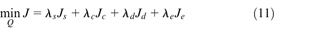
For safe and effective grasping in a dynamic environment, planning algorithms need real-time to deal with changing the target’s movement and obstacles. This paper proposes a new sequential Sense-Plan-Act (SeqSPA) dynamic grasping framework to generate a robot’s real-time and smooth grasping trajectory. Specifically, we cluster all stable grasps of the target, transform the clustering centers into pregrasps, and predict the future motion of the moving objects by using the observed values. The trajectory optimization algorithm constructing the approximative joint space gradient field can generate a smooth trajectory for a 6-DOF industrial robot arm within 2 ms. Our method generates trajectories for multiple pregrasps and selects the time-optimal trajectory for execution. Simulation comparison and actual experiments verify that our framework can immediately respond to environmental changes and efficiently find a grasping trajectory of the near-optimal time. The trajectory optimization algorithm in the framework can also be used alone to generate a real-time grasping trajectory when the prediction module cannot accurately predict the target motion.
Introduction
Many automated tasks require robots to operate objects. Usually, robots operate targets in a static environment with fixed trajectories. However, the robot must generate trajectory autonomously when the environment changes dynamically. For example, in dynamic assembly, grasping and human-machine collaboration, targets and obstacles interacting with the manipulator may move with unknown motion.
Allowing robots to manipulate objects in a dynamic environment can improve the system’s overall efficiency but present more significant challenges. First, motion prediction of dynamic objects becomes extremely important, requiring higher real-time and robustness for visual tracking and prediction. Secondly, the existing grasping planning algorithms filter and sort the grasp poses and only use one grasp to plan a trajectory. In a dynamic environment, especially in the case of moving obstacles, the optimal grasp pose cannot be determined only by a grasping planning algorithm. Due to the change in the external environment, the non-optimal grasp pose may be more conducive to dynamic grasping when considering the whole capturing trajectory. Finally, continuous changes require online and fast motion replanning. With the change in the motion state of the target, we must update the trajectory of the manipulator and grasping pose in real time. Sampling-based algorithms generate random, unstable and fluctuating paths in each replanning, which does not meet these requirements. Optimization-based algorithms consume more time in cluttered scenes and are unsuitable for replanning in a dynamic environment.
Aiming at the problem of existing algorithms, we propose a new dynamic grasping framework in this paper. First, Bézier trajectories are used to predict target and obstacle trajectories. Secondly, ideally, the framework plans trajectories for all grasp poses and selects the optimal trajectory for execution. However, the calculation is heavy, and the trajectories of the similar grasp poses are also close. Therefore, it is necessary to cluster the grasp poses, take each clustering center as the target for trajectory planning, and select the optimal trajectory for execution. Finally, this paper simplified our earlier motion planning algorithm. 1 The trajectory planning module calculates the intersection time, use B-spline curves to represent joint trajectories, and generates smooth, collision-free and dynamically feasible trajectories after nonlinear optimization. The trajectory planner has good real-time performance and can be used in the whole grasping framework or alone. The grasping process for a moving object is shown in Figure 1.
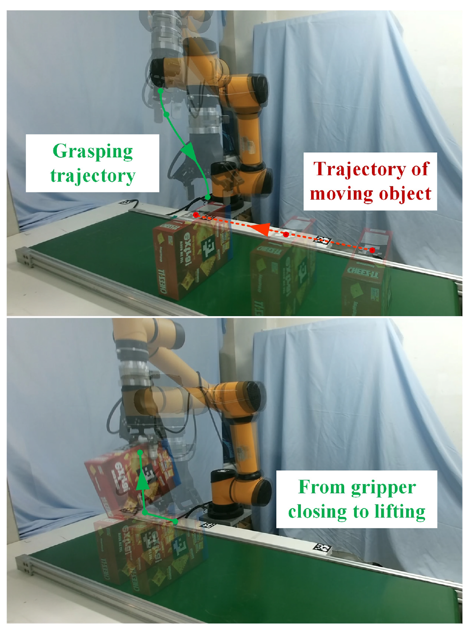
A mechanical arm is grasping a moving object. We online predict the object motion, plan trajectories for multiple pregrasps, and execute the shortest time of the trajectory. The gripper reaches the pregrasp position and then grasps and lifts the object.
The main contributions of this paper are summarized as follows:
This paper makes the motion planner 1 suitable for multi-pregrasps real-time planning. After predicting the intersection time, we construct a joint space gradient field and use nonlinear optimization to calculate the joint trajectory quickly.
This paper proposes a new dynamic grasping framework, which includes a polynomial trajectory prediction module, a grasping planning module, and a trajectory planning module. The framework clusters many grasps into a small number of pregrasps, generates the trajectories of all pregrasps, and selects the optimal time trajectory for execution.
We systematically evaluate the performance of the dynamic grasping framework through simulation and actual grasping experiments, which are multi-target and multi-task, and demonstrate the feasibility and robustness of the framework.
Related work
This section summarizes relevant work in four parts: Grasping in Dynamic Environments, Robotic Grasping, Object Motion Prediction and Motion Planning.
Grasping in dynamic environments
The two mainly alternative system architectures for grasping in dynamic environments are Locally Reactive Control and Sense-Plan-Act.2,3
Locally Reactive Control: Such system architectures do not use global motion planning modules but local strategies to generate real-time reactive motions. 2 They respond immediately to change and are robust to uncertainties in sensors and object motion. Wholly based on feedback control systems4–6 are used in grasping in dynamic environments for a long time. Recently, many studies are based on deep reinforcement learning.7–9 The robotic control policy neural network that uses raw input from a camera is established in Levine et al. 7 A mobile operation control framework 8 based on multi-task reinforcement learning is proposed to achieve universal dynamic target tracking and grasping. In Pham et al., 9 the neural network predicts the action that meets the constraint closest to the unsafe action so that the arm can grasp the moving object while avoiding the obstacle. However, local reactive control may fall into a local minimum in a complex workspace.
Sense-Plan-Act: In the high degree of the freedom robot system, constructing sensing, planning, and action components through strong modularity is still the primary mode. In this system, the perception module builds a complete environment model, the planning module generates a collision-free and optimal trajectory, and finally, it is executed by the precise controller. Systems built around Sense-Plan-Act (SPA) are well suited to structure and well-defined environments. 2 The planner based on graph search 10 is used to generate the trajectory. After the manipulator reaches the pregrasp, the controller is used to grasp in Cartesian space. A search-based kinodynamic motion planning algorithm is presented to generate time-parameterized trajectories to grasp moving objects smoothly in Menon et al. 11 The RRT-Connect method in time configuration space is used in Yang et al. 12 to generate a path to pick up the moving target. Still, it cannot cope with the uncertainty and changing environment. Due to the SPA’s lack of environmental feedback during movement execution, researchers have proposed extensions such as Sense-Plan-Act (SeqSPA). Constant-Time Motion Planning (CTMP) 13 uses real-time heuristic search planning to grasp moving objects in the finite horizon. The Reachability-Aware Grasping and Motion-Aware Grasping are used in Akinola et al. 14 to filter reachable grasps and incorporated the path from the previous timestep to seed the search process to achieve a quicker and smoother trajectory. Compared with SPA, SeqSPA systems still have better-grasping results when there is uncertainty in sensor signal and motion state.
However, the methods in Islam et al. 13 and Akinola et al. 14 cannot quickly cope with the dynamic obstacles. The core reason is that a motion planner requires a longer computing time than a local motion controller, which makes it impossible to react quickly in a dynamic environment. This paper develops a new SeqSPA dynamic grasping framework. The global planner in this paper is fast and can be used as a local motion controller. Moreover, the prediction module increases the reliable length of each trajectory.
Robotic grasping
Methods based on deep learning can directly extract the grasp pose of the target from an RGB-D view15,16 or Point Clouds. 17 These methods collect expensive grasp data sets in the real world to train a neural network. The physics-based simulation method is used in Eppner et al. 18 to evaluate the grasping quality of the parallel jaw and establish a dense data set. The method in Akinola et al. 14 generates robust grasping data sets through physical simulation, and uses pre-calculated reachability space 19 and motion intention neural network to evaluate feasible grasp poses. In this paper, a stable grasping dataset is generated by physical simulation, the same as Eppner et al, 18 and the clustering algorithm reduces the similar grasp poses.
Object motion prediction
The use time of the optimized trajectory can be improved by estimating the future motion of the target through the prediction module. The target pose detection system uses Kalman and Buey filtering methods20–22 to filter the noisy pose results into more stable values. However, it is unreliable to use rough motion models to estimate the motion of future targets. The Covariant Optimization is utilized in Jeon et al. 23 to consider the target motion prediction of collision, and the collision term needs much time to calculate. The polynomial regression to predict object motion and generates a corresponding trajectory through the constraint-free QP optimizer is adopted in Chen et al. 24 Fast-Tracker25,26 improves this method by using Bezier curves to represent the target prediction trajectory, and adding dynamic constraints and time-varying confidence in the optimization. We use this method to predict the movement of all objects.
Motion planning
The process of motion planning usually consists of path search and trajectory optimization. Sampling-based methods12,27,28 and search-based methods10,11,13,14,29 are the main ways of front-end path search. The front-end path is jerky and leads to wavy motion. The back-end trajectory optimization algorithm calculates a smooth trajectory with time parameters based on the front-end path. The back-end methods of the manipulator30,31 can optimize a satisfied constrained trajectory, but the optimization process does not consider the obstacles. CHOMP algorithm 32 introduces the Euclidean Signed Distance Field (ESDF) information into motion planning to optimize trajectory using workspace gradient information. STOMP algorithm 33 uses sampling technology to generate multiple alternative trajectories and obtains the optimal trajectory through multiple iterations and evaluation of the cost of candidate trajectories. Machine learning techniques34,35 are used to optimize trajectories. The clearance estimation is used for motion planning in Chase Kew et al., 34 but the algorithm cannot quickly and adaptively handle dynamic obstacles. The method in Fujii and Pham 35 can quickly smooth the trajectory while processing dynamic obstacles but must obtain an initial collision-free path in advance. EGO algorithm 36 establishes a gradient field for a UAV without ESDF and uses the properties of the B-spline curve for rapid trajectory optimization.
Problem definition and algorithm framework
The task simulates a scenario in which multiple objects are placed on the conveyor belt in a warehouse. 14 The robot arm must avoid colliding with non-target objects on the conveyor belt or static obstacles around it and pick up the target object. In grasping, there will be an external human being or robot as a moving obstacle or the conveyor belt speed mutation. We assume that we know the models of the target objects and obstacles, but their motions are unknown. The robot must catch and lift the target without colliding with surrounding obstacles.
We propose the manipulator dynamic grasping system, as shown in Figure 2. The SeqSPA Dynamic Grasping Frame is presented in Alg.1. Our method first extracts the pre-computed grasp data
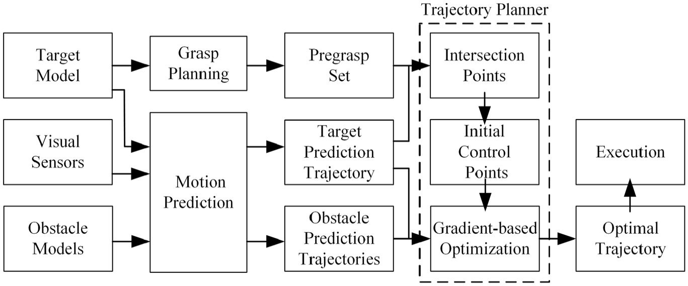
Dynamic grasping system architecture diagram. The predicted trajectories of the target and obstacles generated by the motion prediction module and the pregrasp poses generated by the grasp planning are input into the trajectory planning module to generate the optimal trajectory. When using the motion prediction model, if there is a significant error between the actual position of the target and the predicted position, or the obstacle’s latest predicted trajectory will collide with the manipulator, the framework carries out the planner again. When not using the prediction module, the planner uses the current target and obstacles positions to generate the trajectory at a specific frequency.
Convert all initial trajectories to the B-spline control points
Grasp planning
We used an approach similar to Akinola et al. 14 and Eppner et al., 18 where a grasping database is precomputed while all target objects remain static, to collect data in the physical simulation. First, many dense samples are taken to generate the grasp poses on the object’s surface. Then the object is lifted 20 times in the physical simulation environment, with random noise added each time. The success rate is the selection measure of the reliability of each grasp pose. The first 600 grasps are used as the grasping dataset.
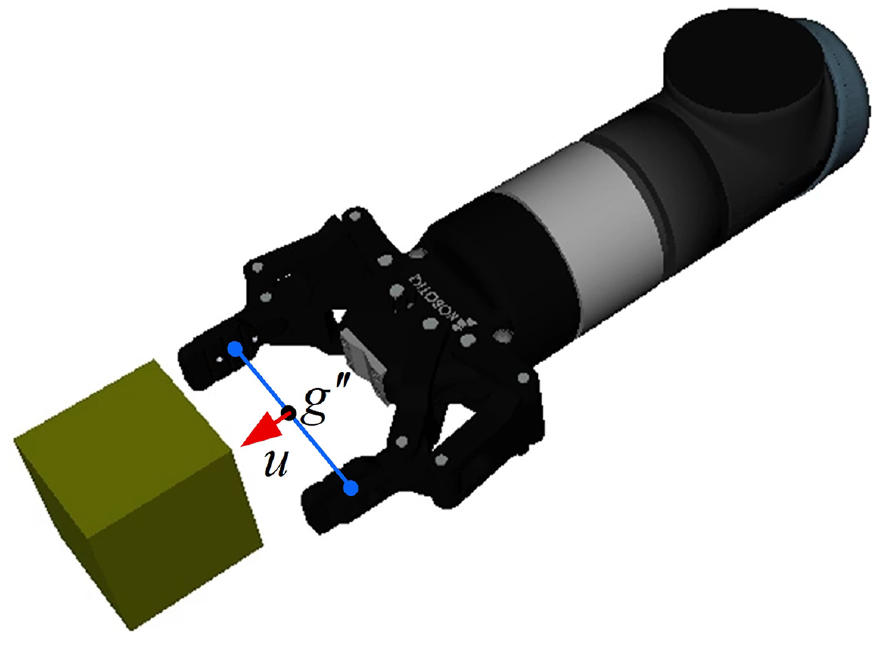
We use the widely used 4-dimensional grasp representation in the physical simulation to represent the object grasp configuration. The four dimensions are: grip width w, opening size l, grasping position g and orientation u. We use a model the same width w as the actual gripper in the simulation. We sample on the target object’s surface, and the intersection point with the other side of the object is found through the normal line corresponding to the sampling point. The two points’ connection length is l, and the center point coordinate value of the segment is g. The gripper takes the line between two points as the rotation axis and samples in [−pi/3, pi/3] around the axis as u.
Our evaluation metric is based on distances between grasps and does not consider w and l. A grip pose

where
We use the K-Means to aggregate the robust grasps into k classes, where k = 10. In K-Means, the initial cluster center is randomly generated, and the distance between each sample and each cluster center is calculated by
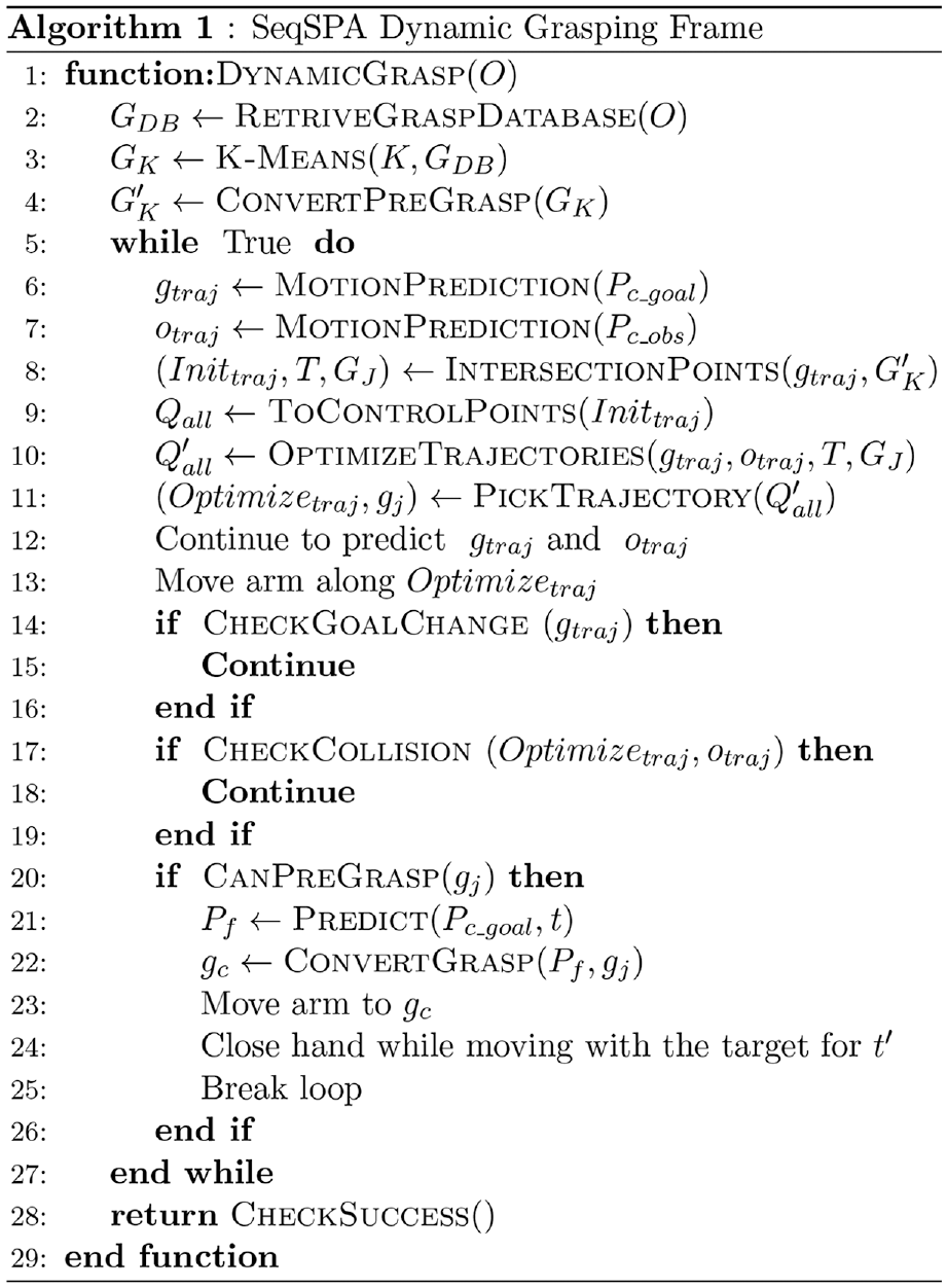
The transform relationship between the grasp and the pregrasp is shown in Figure 3. The center of the gripper at the grasp pose with closed gripper is g, and the center of the gripper after opening is
The transformation relation between grasp and pregrasp. (a) is the position after the gripper is closed, which is one grasp in the grasps database including grasping orientation u, gripper center g, and the distance
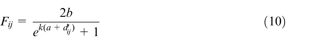
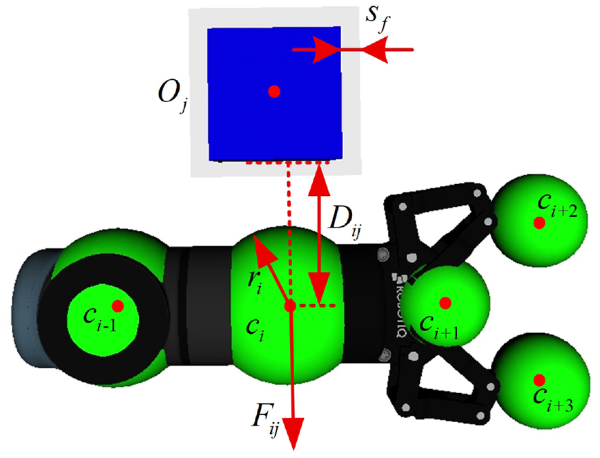
Since there are moving obstacles around the target, we conduct collision detection on the gripper, part of the arm and the obstacle, in which the gripper is in the pregrasp, as shown in Figure 4. We use a metric to rank the collision-free pregrasps. Our metric can be defined as:

The mechanical arm components for collision detection in the grasp planning.
where
Using f to arrange the candidate data from small to large, the first data is the best pregrasp at this moment.
Motion prediction
The planner needs time to calculate trajectories, quickly becoming obsolete as the object moves. Therefore, predicting the future pose of the target can improve the task’s overall success rate. We adopt the Bézier curve
The method in Pan et al.
26
maintains a queue
The cost function minimizes the residual distance between the observation data and the prediction trajectory 26 :
Where,
The Object-oriented software for Quadratic Programming 37 is used to solve the optimization problem of the Bézier curve that meets the velocity and acceleration constraints in Han et al. 25 and Pan et al. 26
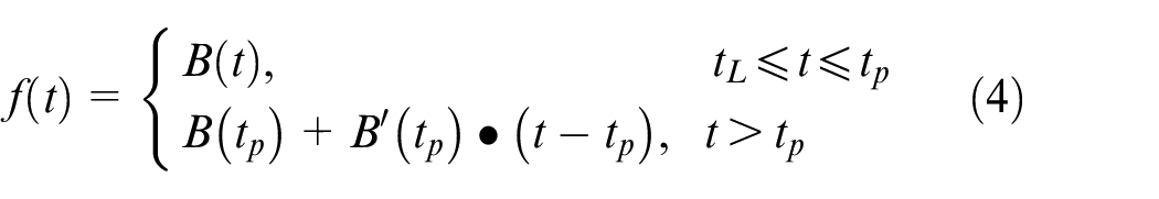
Our complete motion predicted trajectory is shown as follows:
We set
Motion generation
When grasping a dynamic object, the movement of the end-effector can be divided into four stages: pregrasping, grasping, tracking, and lifting. The manipulator reaches the pregrasp pose, approaches the grasp pose, closes the gripper while tracking the target, and lifts it. Our previous algorithm framework 1 is the SPA system. The trajectory generation algorithm to reach the pregrasp position contains sampling-based path search and nonlinear trajectory optimization. To further improve the computational efficiency of trajectory generation in our framework, this paper removed the time-consuming front-end sampling algorithm and trajectory feasibility adjustment module. When a trajectory falls to a minimum or the velocity and acceleration of the trajectory are not feasible, we remove it directly. This paper carries out real-time trajectory planning with multiple grasping poses. Removing several infeasible trajectories does not affect the grasping task.
We first estimate the intersection position using the rapid generation of motion primitive algorithm in Mueller et al. 38 according to the position and speed of the end-effector and the target. Then the planner generates multiple trajectories using the gradient-based method and selects the optimal trajectory for execution. We use the Cartesian controller to move the mechanical arm during the grasping, tracking and lifting stages.
Estimate intersection point
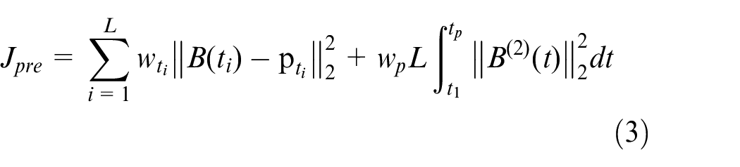
Assuming no obstacles, we need to calculate an optimal intersection trajectory to grasp the moving target. The total initial trajectory cost function
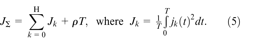
Where,
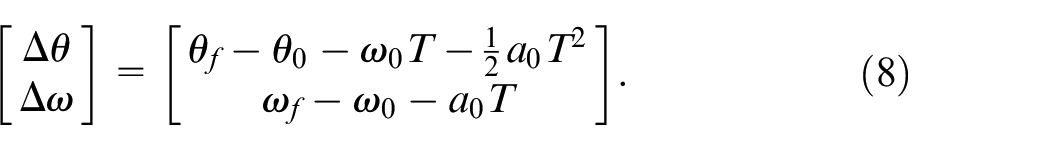
By using Pontryagin’s minimum principle, fixed trajectory end angle and angular velocity, the optimal state trajectory can be straightforwardly solved 38 :
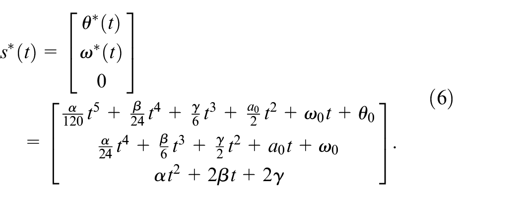
Assuming the initial angle, angular velocity and angular acceleration of the
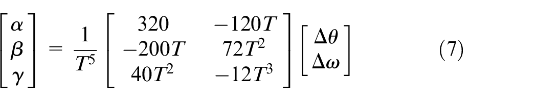
Where
Each joint cost value 38 can be calculated as follows:
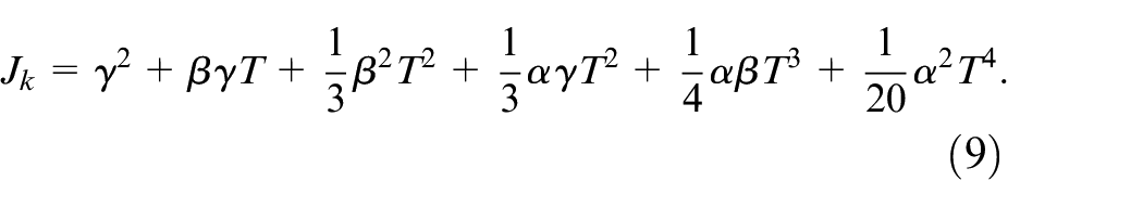
The only variable in the expression of
We sample the path points along the target’s predicted trajectory starting from the starting point. The target center sampling point
Gradient-based trajectory optimization
Due to ignoring obstacles’ information in the manipulator workspace when calculating the initial joint trajectory, the initial trajectory is close to or through obstacles. Therefore, we transform ESDF information into the joint space and use nonlinear optimization to generate smooth, safe and kinematically feasible trajectories in a short time.
This paper uses the method in Wei et al. 1 to establish the approximate repulsive gradient field generated by obstacles in high-dimensional space. Thus, we establish the distance and gradient expressions between the path point and a single obstacle in joint space for the collision penalty.
Our planner uses robotic control points to optimize the trajectory and the oriented bounding boxes (OBB) for collision detection. The distribution is shown in Figure 5. As shown in Figure 6,
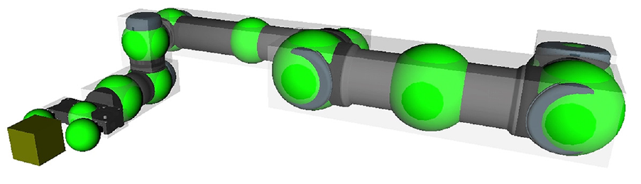
The distribution of control points (green points) and oriented bounding boxes (transparent cubes).
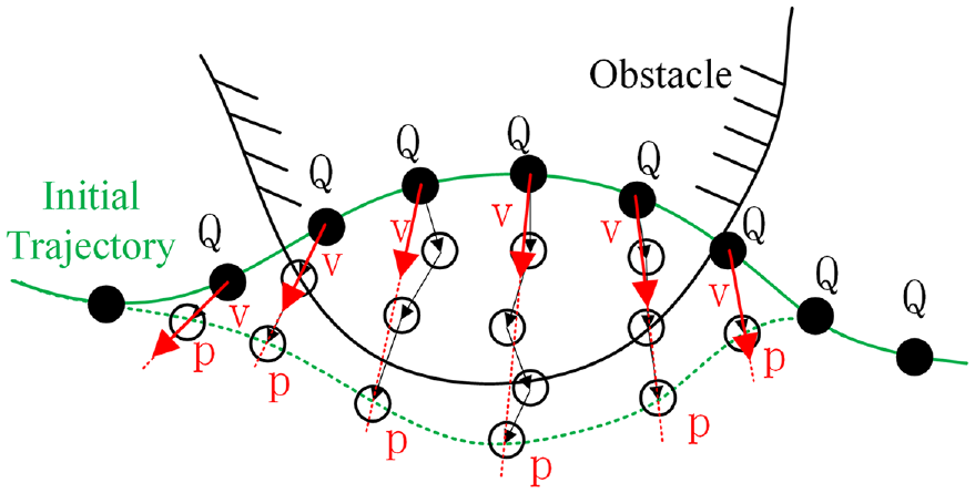
The repulsive force generated by the obstacle on the control point.
where
We calculate the repulsion force of each control point, convert the repulsion force to the origin of the corresponding connecting rod coordinate, and combine the force and torque values. Repulsive force and torque at the origin of the coordinate affect the joint coordinates from this link to the base. The force and torque at the origin of each link coordinate system are recursively deduced to the base coordinate system by using the recursive formula of force and torque in the series mechanism of robotics. In this manipulator configuration, the torque values
Repulsive torques will move the manipulator away from the obstacle.
Approximate repulsive gradient field was represented by
The establishment process of
We use nonlinear optimization method to plan uniform B-spline curve control points.39,40 The derivative of a B-spline curve is also a B-spline curve, whose convex hull characteristics can ensure dynamic feasibility and safety. The cost function is as follow:
where
In order to successfully grasp the moving object, the gripper needs to reach the pregrasp accurately and has the same speed as the target. When no end-point penalty is imposed, optimizing the penalty function of the first several terms will change the control points for determining the terminal position and velocity. So, we add the end trajectory point constraint to reduce the deviation of the manipulator reaching the pregrasp pose after optimization. The function is defined as follows:

where
where

Implementation details and results
We experimented with the simulation environment and the actual robot to evaluate our method. In the simulation, we evaluate the performance of our algorithm in different tasks for different targets. The simulation environment includes the target’s random linear or nonlinear movement, whether there are static obstacles, obstacle with the same speed as the target, and external moving obstacles. Then, the algorithm’s feasibility is verified by typical working conditions in the real world with different targets.
L-BFGS 41 is a quasi-Newton Algorithm to solve the nonlinear optimization problem. The dynamic grasping framework runs on a standard desktop computer with a single-core CPU of 3.20 GHz, Intel Core i7-8700, through Ubuntu 18.04 and ROS melodic.
Experimental setup
According to the actual task and previous experience, 14 we design seven working conditions to evaluate our method on the UR5-Robotiq robots, and the specific settings are as follows:
Linear Motion: The target moves uniformly in a straight line on the conveyor belt with no obstacles around, as shown in Figure 8(a). We random set
Linear with Static Obstacles: In the Linear Motion scene, we divide the near region surrounding the robot into three regions, as shown in Figure 8(b). We place one obstacle in each area and randomly locate the obstacle’s position in each region.
Linear with Moving Obstacle on The Belt: In the Linear Motion scene, we place an obstacle around the target that moves at the same speed as the target, as shown in Figure 8(c).
Linear with External Moving Obstacle: As the arm grasps the target in the Linear Motion scene, the external moving obstacle sweeps over the conveyor belt, as shown in Figure 8(d). The moving obstacle speed is about 0.05–0.15 m/s and changes dramatically some times. The height of the obstacle track to the conveyor belt surface is 0.2–0.8 m.
Linear with All Obstacles: In the Linear Motion scene, we add one static obstacle, one obstacle at the same speed as the target, and an external moving obstacle, as shown in Figure 8(e). The distribution and velocity of the three obstacles are the same as tasks (2)−(4).
Linear with Varying Speed: In the Linear Motion scene, the target object’s speed will change dramatically 3–5 times, and the linear velocity range is 0.05–0.1 m/s.
Circular Motion: The object moves uniformly around the manipulator’s base, as shown in Figure 8(f). The target trajectory radius is
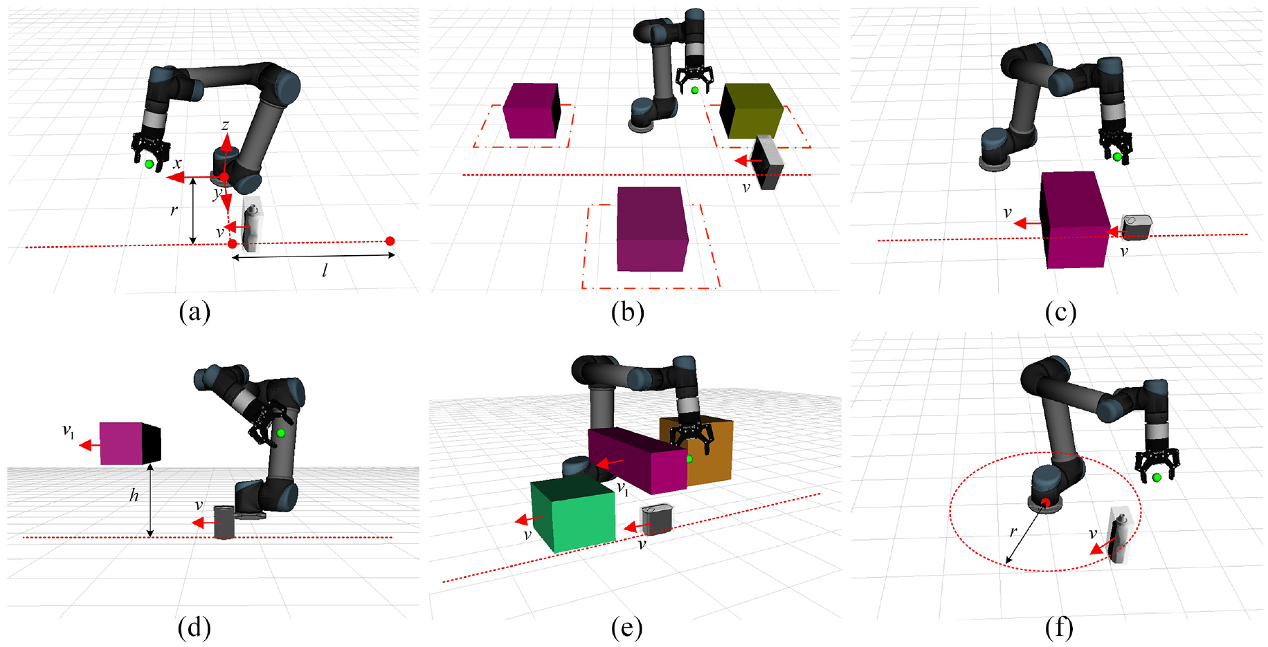
Schematic diagram of random experimental motion parameters in seven working conditions. Schematic diagrams of working conditions 1–5 are (a)–(e), random parameters of working conditions 6 and 1 are the same, and (f) corresponds to working conditions 7. The distance between the target trajectory and the base coordinate is r. l is the projected length of the target starting point to the base along the conveyor belt direction. v is the target motion velocity. When the target moves in the x-axis’s positive direction, v is positive.
We selected five grasping targets and generated pregrasps, as shown in Figure 9. Each target’s initial stable grasp poses are about 600, and the clustering algorithm sets 10 classes. The grasps, after clustering, are transformed into pregrasps. All objects are used for the simulation and the actual robot experiment. Five kinds of targets are captured in each simulation experiment scene of each method. We run 40 times for each object in one scene and count the average success rate and capture time of 200 tests.
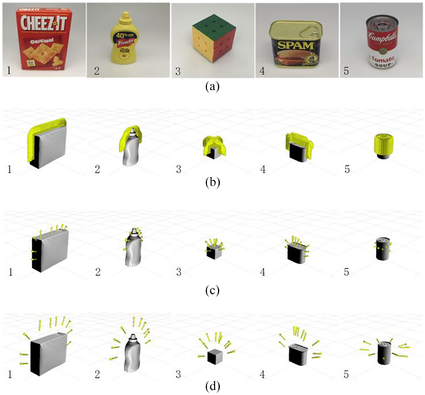
The graspable objects and corresponding pregrasps. The five graspable objects from the YCB Object Database 42 are shown in (a). Many stable grasp poses for five targets are shown in (b). In (c), the grasp poses are clustered, and 10 grasps are generated for each target. The grasps transform into the pregrasps in (d): (a) five graspable objects, (b) stable grasps, (c) grasps after clustering, and (d) pregrasps.
We compare the performance of the below methods in the experiment:
OUR: This is our complete framework. We removed the trajectories with the speed and acceleration exceeding the limit in the obtained trajectories and selected the trajectory with the shortest time for execution.
One grasp: Unlike OUR, this method only uses one grasp with the lowest score for each plan and runs the calculated trajectory. When the first planning fails, we rerank the pregrasps and carry out the trajectory optimization again.
No prediction: This method removes the prediction module to study its importance. It does not predict the trajectory of the target and obstacles but directly plans the trajectory of all pregrasps at the moment and selects the trajectory with the shortest time for execution. The planner takes an average of 2 ms to generate trajectories from the starting position. When the end-effector is close to the target, the trajectory length will decrease, so each planning time of a single trajectory is less than 2 ms in the grasping process. Therefore, the maximum time for each plan should not exceed 20 ms. The planner is used as a controller, and the control rate is about 50 Hz.
No prediction + One grasp: This method removes the prediction module and uses one grasp with the lowest score. Only one trajectory is generated per planning. The planner is used as a controller, and we set the control rate to be 100 Hz.
Experimental results
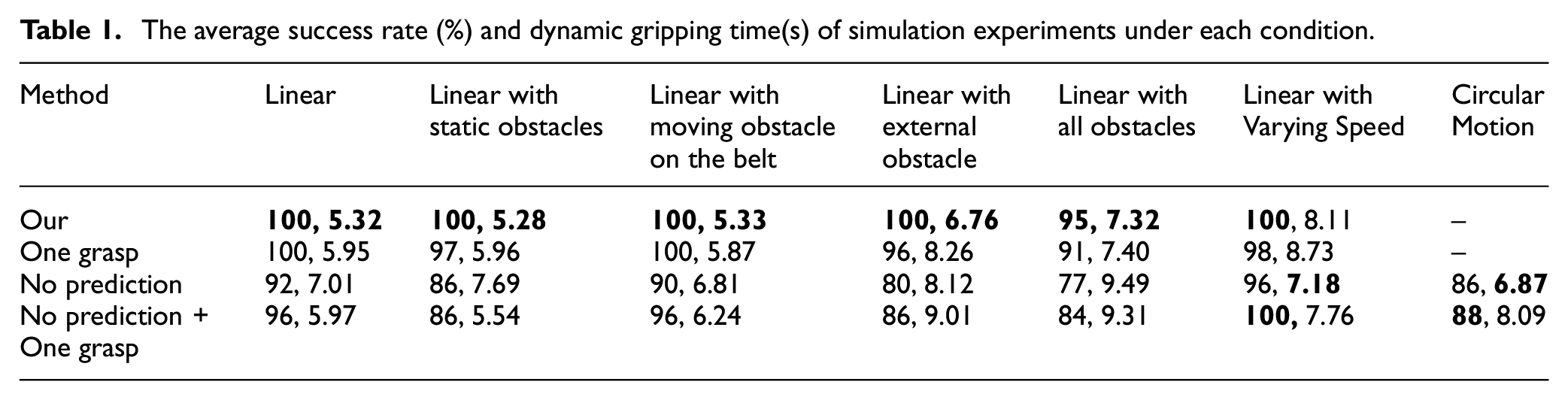
The simulation results are shown in Table 1. The bold entries are the best results of the success rate and dynamic gripping time among the four methods Under working conditions 1 and 5, planning trajectories generated by different algorithms are shown in Figures 10 and 11, respectively.
The average success rate (%) and dynamic gripping time(s) of simulation experiments under each condition.
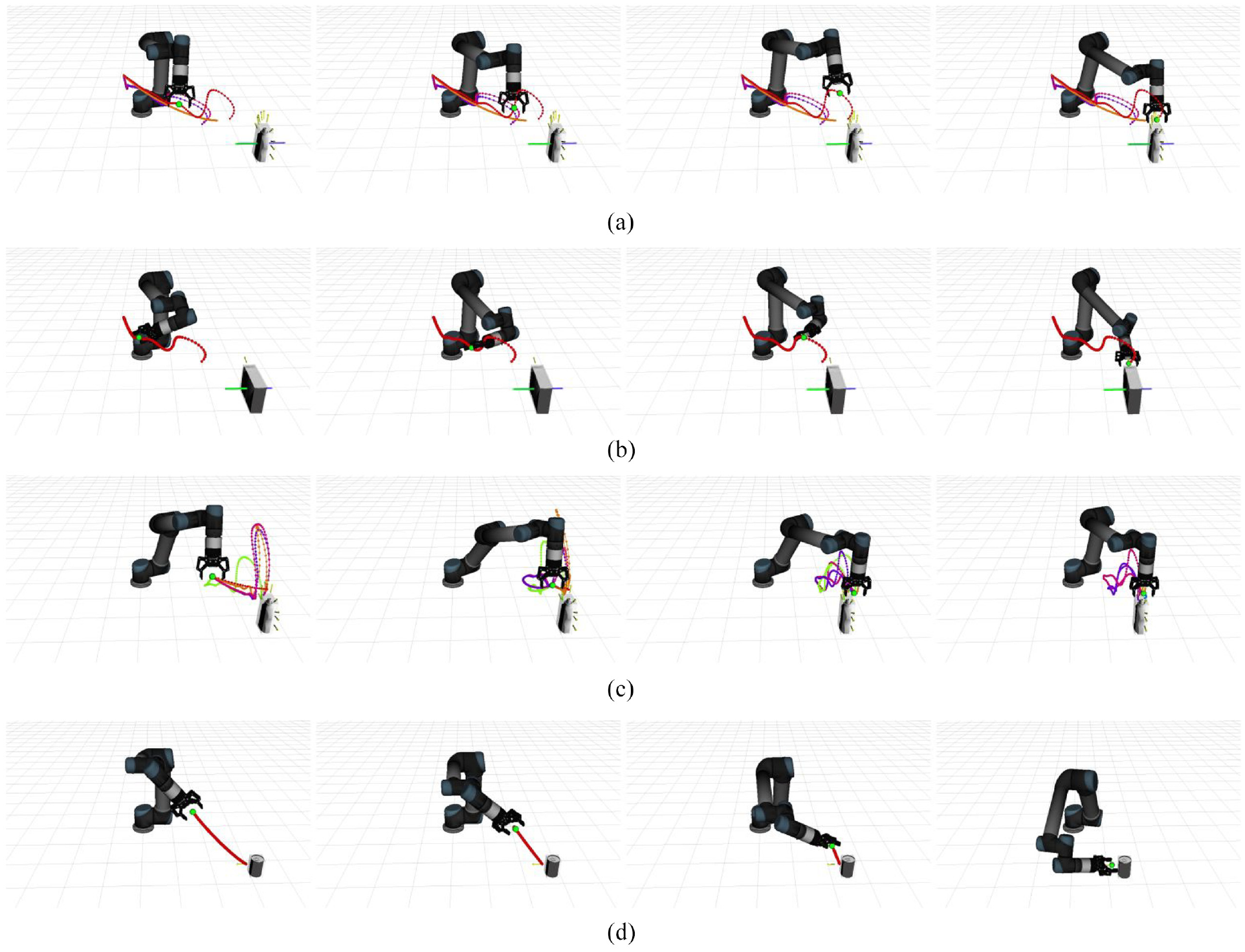
Trajectories generated by four algorithms in working condition 1. The yellow arrows near the object are the selected pregrasps. In task 1, the target is moving uniformly on the conveyor belt. Algorithms 1,2 contain the prediction module and plan the trajectory at one time. The green trajectory at the geometric center of the target object is the prediction trajectory, and the blue trajectory is the historical trajectory, as shown in (a)–(b). Algorithms 3, 4 do not include the prediction module and carry out real-time trajectory planning, as shown in (c)–(d). Algorithms 1 and 3 plan trajectories for all grasp poses and generate multiple feasible trajectories.
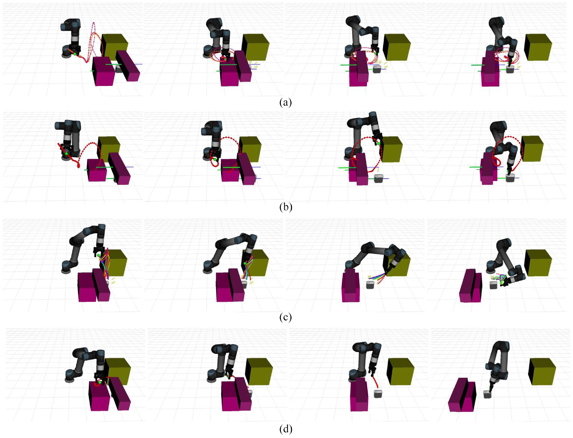
Trajectories generated by four algorithms in working condition 5. The target and the obstacle in front are on the conveyor belt in uniform motion, one obstacle is above the target and moves in a straight line with variable speed along the conveyor belt, and one static obstacle is on the right side of the manipulator. Algorithms 1, 2 contain the prediction module to predict the trajectory of all moving objects and generate a long-term trajectory. However, when the velocity of the outside moving obstacle changes to lead original trajectory colliding with the obstacle in the future, the planner carries out again to generate a new trajectory, as shown in (a)–(b). Algorithms 3 and 4 carry out real-time trajectory planning, as shown in (c)–(d). Before the planning, the grasping planner sorted the grasps and eliminated the grasps where collisions occurred. Therefore, in (a) and (c), the target only has eight pregrasp poses. In (d), real-time trajectory planning selected the nearest pregrasp to the gripping jaw, so the pregrasp changes in real-time.
In working conditions 1–5, the conveyor belt velocity is unknown but fixed, and the trajectory prediction module can better predict the target trajectory. Among them, in conditions 4 and 5, the movement state of the obstacle changes in real-time. Algorithm 1 generates multiple trajectories and finds the one with the shortest execution time. The success rate of algorithm 1 is slightly higher than algorithm 2, much higher than algorithms 3 and 4, and the grasping time of algorithm 1 is closer to the global minimum. Compared with Algorithm 3, Algorithm 4 uses only one pregrasp, so the trajectory update frequency of Algorithm 4 is faster, and the success rate is higher. When the environment is entirely predictable, each execution of the local shortest path is not the entire shortest path. Therefore, algorithms 3, 4, which updated the trajectory in real-time, has a longer grasping time than algorithms 1, 2. In condition 5, with the most obstacles, algorithms 3 and 4 are only planned for the current environment, so they easily fall into local extremums and have the lowest grasping success rate.
In case 6, the speed of the conveyor belt will mutate several times, and algorithm 1 can only calculate the shortest grasping time at the speed of the conveyor belt at this moment but cannot calculate the global shortest time. The grasping time of algorithms 3, 4 is shorter than 1, 2. Thus, the real-time trajectory update algorithm has a shorter grasp time in an unpredictable environment. The success rate of algorithms 1, 2 and 3, 4 is similar, demonstrating our overall algorithm framework’s real-time performance and robustness.
The target moves in a circle, and its speed constantly changes in condition 7. In algorithms 1 and 2, the manipulator’s predicted intersection point is not on the target trajectory circle. The Bezier curve used only has a predicted length of 1.5 s. When the time is more significant than 1.5 s, the position can be predicted according to the speed at the end of the Bezier curve and the predicted trajectory is a straight line, as shown in equation (4). When the initial intersection time is greater than 1.5 s, the intersection point will be on the straight line instead of the Bezier curve and the prediction error is large. So the grasping success rate is low, which is not compared in Table 1. Algorithms 3 and 4 generate real-time trajectories and can respond to changes immediately, and they also have a high grasping success rate in condition 7. In working conditions 6 and 7, the environment cannot be completely predicted. Algorithm 3 updates the trajectory in real time and executes the shortest one among multiple trajectories each time, so the overall time is the shortest.
In summary, when the target trajectory can be predicted, our algorithm framework can respond immediately to environmental changes and has the highest success rate. When the target trajectory cannot be accurately predicted, algorithms 3 and 4 generate the real-time trajectory, while algorithm 4 has a faster calculation speed and higher success rate. However, algorithms 3 and 4 may fall into local extreme values in a complex environment with many obstacles, such as task 5.
Real robot grasp
As shown in Figure 12, the experimental platform consists of an AUBO-i5 manipulator, a parallel gripper, a conveyor belt and a Kinect2 depth camera. The camera in front of the conveyor belt is used to collect visual information. Based on the simulation experiment results, we selected algorithms 1 (Our) and 4 (No prediction + One grasp) for the real-world experiment, and the target objects are the same in the simulation experiment. We add a position based visual servoing (PBVS) controller for comparison of algorithms. Based on the target information collected by the camera, the difference between the end pose of the current manipulator and the target pose is obtained. The servo controller is used to calculate the motion speed of the manipulator. Then the motion speed of each joint of the manipulator is obtained to drive the manipulator to approach the target.
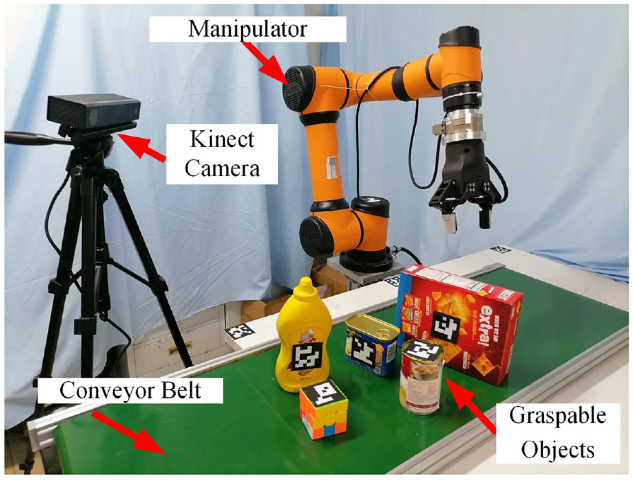
The experimental platform.
We use three tasks in the actual experiment. In the Linear Motion and Linear with Moving Obstacle on The Belt tasks, the conveyor belt speed does not exceed 0.1 m/s. In the Linear with Varying Speed task, the linear velocity range is 0.02 to 0.1 m/s, changing the belt speed three times. We test each object 10 times in a task, resulting in 50 times for each algorithm.
The experimental results are shown in Table 2. The bold entries are the best results of the success rate and dynamic gripping time among the three methods. The conveyor belt velocity is unknown in the first two tasks but does not occur mutation. In the Linear Motion task, algorithm 1 uses a prediction module to generate a long trajectory with a higher success rate. As the trajectory with the shortest time is executed every time, the grasping time is the fastest. The PBVS method responds quickly and has the highest success rate. In the Linear with Moving Obstacle on The Belt task, algorithm 1 has the highest success rate and takes the least time. Due to the not complicated environment, algorithm 4 will not fall into the extreme value. However, the PBVS method moves directly to the target in the workspace and cannot avoid obstacles, so the success rate is the lowest. In the Linear with Varying Speed task, The PBVS algorithm achieves the highest success rate and takes the least time. Algorithms 1 and 4 have similar success rates.
The average success rate (%) and dynamic gripping time(s) of real-world experiments under each condition.
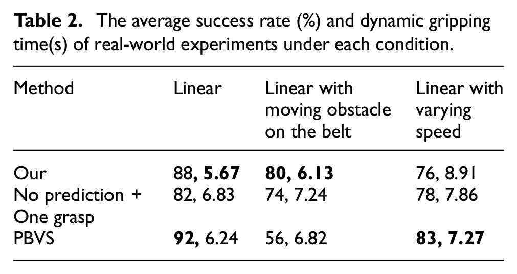
Overall, our algorithmic framework (Algorithms 1) generates complete trajectories and works best in the presence of obstacles. When the target moves regularly, algorithm 1 calculates the intersection position in advance, making the grasping time the shortest. PBVS is a local reactive control method that works best when there are no obstacles, and the target velocity varies greatly. Algorithm 4 generates the complete trajectory in real time, and the performance is between algorithm 1 and PBVS. In the Linear with moving obstacle on the belt task, the dynamic grasping process of the target moving at a speed of 0.09 m/s on the conveyor belt is shown in Figure 13.
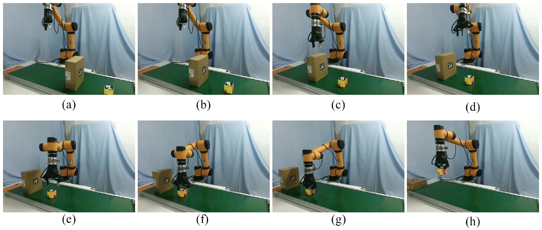
The actual robot captures the moving object while avoiding an obstacle. We place the target and obstacle on the unknown speed conveyor belt. The prediction module records the target’s location information for a period to predict the target trajectory, as shown in (a)–(b). The robot arm executes the corresponding trajectory and arrives at the pregrasp pose in (c)–(e). After reaching the grasp pose, the robot closes the gripper and lifts the target object in (f)–(h).
Conclusions
This paper proposes a new dynamic grasping framework for effective grasping in a dynamic environment. Many grasp poses of the target are clustered to determine multiple pregrasp poses, and we use the Bézier curve motion prediction module to generate predicted trajectories of all moving objects. The trajectory optimization algorithm constructing an approximate gradient field in joint space can generate a smooth trajectory. Simulation comparison and actual experiments verify the dynamic grasping framework’s high performance and feasibility. The algorithm framework is robust to environmental changes and has a high success rate in complex environments. When the target’s motion state can be accurately predicted, we can achieve fast and robust moving target grasping using the prediction module and trajectory planning for all grasp poses. When the environment is not easy to predict, we only quickly plan for the current optimal grasp pose and do not use the prediction module, which can also get good results.
In the future, we will use deep learning to establish the mapping relationship between the deep image features and the manipulator’s local trajectory and use deep reinforcement learning to train the dynamic grasping framework. The new method will combine the prediction and planner modules to achieve more efficient dynamic grasping.
Footnotes
Declaration of conflicting interests
The author(s) declared no potential conflicts of interest with respect to the research, authorship, and/or publication of this article.
Funding
The author(s) received no financial support for the research, authorship, and/or publication of this article.