
Abstract
The article considers a method of examining the influence of dynamic couplings contained in the underwater vehicle model on the movement of this vehicle. The method uses the inertia matrix decomposition and a velocity transformation if the fully actuated vehicle is described in the earth-frame representation. Based on transformed equations of motion, a controller including dynamic couplings in the gain matrices is designed. In the proposed method, the control algorithm is used for the test vehicle dynamics model taking into account disturbances. The approach is useful for simulating the model of an underwater vehicle and improving it, thus avoiding unnecessary experiments or planning them better. The procedure is shown for a full model of an underwater vehicle, and its usefulness is verified by simulation.
Introduction
Building a mathematical model of a submersible vehicle is quite a challenge because different aspects of the vehicle itself as well as the environmental impact must be taken into account. Moreover, the equations are strongly nonlinear what leads to their very complicated form. Problems related to modeling have been repeatedly considered in the literature. 1 –3
The presented approach is limited to underwater vehicles for which all input signals are accessible. In many references, such model is considered. Examples of such marine systems can be found. 4 –9
Many control algorithms are expressed in the earth-fixed representation, as in the literature. 2 –4,6,8,10 –12,14,15 Various types of sliding mode control (SMC) algorithms were considered, among others, in the literature. 6,8,11,13,15 –17 However, different tracking strategies are successfully applied, for example, based on backstepping technique, 18 gain scheduling control theory, 19 bio-inspired neurodynamics approach, 20 so-called RISE algorithm 10 or control approach using an observer, 21 adaptive recurrent neuro-fuzzy control, 22 neural network control, 23 and an output feedback control, which use a vehicle model. 24 In the current literature, more other control algorithms can be found, for example, combination of fuzzy logic, genetic algorithm, and SMC, 25 model predictive control, 26 a method in which the port-Hamiltonian theory is applied, 5 combination of recurrent neural network and receding horizon optimization, 27 combination of SMC and backstepping, 14 and backstepping active disturbance rejection control. 28
The problems discussed in this article concern the model-based algorithm in the earth-fixed representation and six degrees-of-freedom (6DOF) fully actuated vehicles. Such algorithms have been developed in the past many times. The comparison study among several controllers from many years ago is well known. 4 One of the controllers was realized in the earth-fixed frame. If the dynamic parameters are known exactly, there is no need to compensate them by restoring generalized forces. In a real situation, however, this is impractical, which is a disadvantage of this algorithm. In the literature, 8 an algorithm was proposed in which continuous input signal chattering effect is alleviated. The controller was robust to model uncertainties. However, rather rarely used closed-loop fractional-order system was considered and only Hölder disturbances were taken into account. The control scheme presented by Fischer et al. 10 was applied to compensate for uncertain, nonautonomous disturbances for a class of coupled, fully actuated underwater vehicles. The approach led to semiglobal asymptotic tracking. An important advantage was the experimental validation of the method in controlled and open-water environments. The disadvantage was larger orientation errors in the open-water test. Due to the lack of simulation tests, it is impossible to relate the results obtained during the experiment to the simulation results. An effective adaptive second-order fast nonsingular terminal SMC strategy for the trajectory tracking of fully actuated autonomous underwater vehicles (AUVs) was given in the literature. 13 The dynamic uncertainties and time-varying external disturbances were taken into account. Simulations for two vehicles were performed. However, the approach seems to be complicated and dynamic couplings in the tested model were not significant. Another solution was the computed-torque controller together with fuzzy inverse desired trajectory compensation technique using a robust adaptive fuzzy observer to control underwater vehicle subject to uncertainties described in the literature. 12 Various simulation cases were considered to show the benefits of the proposed control strategy. However, the dynamic couplings in the vehicle model used were not very strong. A combination of the SMC method with backstepping and nonlinear PD controllers was considered in the literature. 14 The control scheme was verified in a real experiment in various scenarios but some constant disturbances were applied only. Moreover, the most important problem was to introduce an observer to improve the performance of the backstepping technique and the PD controller. A chattering-free SMC for the trajectory control of remotely operated vehicles was introduced by Soylu et al. 15 The advantage was a replacement of the conventional, discontinuous switching term by an adaptive term. Additionally, the neural networks were used to solve the issue of faulty thrusters and thruster saturation limits. The influence of the vehicle dynamics on its movement was not analyzed. The control algorithms are designed primarily from the point of view of their efficiency and performance, robustness to parameter changes and disturbances, but without examining the influence of dynamic couplings. The performance of the proposed controllers is compared with the performance of other algorithms designed to achieve the same goal.
Remark. The subject of this work is the analysis of vehicle motion using a controller that contains dynamic parameters of this vehicle with dynamic couplings. The results of simulation tests are then compared with the results of the controller, which does not contain dynamic parameters or couplings in the gain matrices. The problem considered here concerns therefore the analysis of the effects of dynamic couplings and the influence of dynamics on the motion of the vehicle when its model is known. In this work, models from the literature 2,3 were selected, because they are often used and are very well suited for the application of velocity transformation and to show the advantages of the proposed method of analyzing the dynamics of underwater vehicles.
In this article, a procedure is presented to study the motion changes of an underwater vehicle using a trajectory tracking controller, which contains the dynamic parameters in gain matrices. This means that at the same time, not only the control task is carried out but also obtains information about the effects of the dynamic parameters on the behavior of the vehicle in motion. The proposed method consists of two stages: (1) designing a controller that contains the system parameter set in the gain matrices and (2) dynamics analysis based on a comparison of the tracking control algorithm with a reduced controller that does not contain dynamics in these matrices. To find a suitable control algorithm, the velocity transformation method described by Loduha and Ravani 29 was used, which consists in decomposition of the inertia matrix. Then, for the transformed motion equations, a control scheme for tracking a desired trajectory was proposed. This scheme is expressed in terms of generalized velocity components (GVCs) and it contains in the gain matrices the vehicle dynamics including couplings between variables. Simulation results obtained with the GVC controller are compared with the results of the classical (CL) algorithm, in which the control gain matrices do not depend on dynamical parameter set. An important value of this method is to estimate, by means of a simulation, the effect of the dynamics and couplings contained in the vehicle model on the behavior of the system based on the response from the GVC and CL controllers to track the desired trajectory. An additional advantage of the GVC controller is that its response, due to the dynamic parameters contained in the gain matrices, is closely related to the vehicle dynamics.
Compared with the literature, 30 this work is characterized by the following differences: (1) the decomposition method used here is different, and consequently, the analysis provides complementary results to the method given in the literature 30 ; (2) the physical interpretation of variables is easier because we use the same units both in equations expressed in terms of the GVC and in CL-based equations, which is the difference from the cited work; and (3) based only on the test proposed in the literature, 30 we obtain indirect information about the behavior of the vehicle (the decomposition method used here leads to obtaining of the GVC set, which corresponds to the method described in the literature 29 but in the vehicle external frame).
The remainder of this article is organized in the following way. The equations of motion in terms of the GVC for an underwater vehicle are presented in the second section. The third section shows the control algorithm and scheme of the dynamics test. Numerical simulations illustrating effectiveness of the approach are given in the fourth section. The fifth section contains conclusions.
Transformed equations using generalized velocity component
Modeling real underwater vehicles is difficult due to the system itself and the physical phenomena, including environmental disturbances, that occur. Therefore, the model is always only an approximation. Additionally, the equations of motion are highly nonlinear and many physical phenomena are only partially covered. There are various methods of modeling the dynamics of a system and analyzing its properties. Some of these methods may even lead to a deeper analysis of the behavior of the system. Problems concerning the modeling of marine vehicles have been considered in many works, among others in the literature. 1,31 –34
Since the aim of this article is to show usefulness of the equations of motion expressed in the GVC, the model should be general but also simplified enough to be suitable for the design of vehicle controller. In the proposed approach, the analysis of the dynamics and the influence of couplings are performed using the description in quasi-velocities, which are obtained from the decomposition of the inertia matrix. The result of this transformation is the inclusion of dynamic parameters (mass, geometrical, etc.) into the controller gain matrix. Then, the information about the dynamic effects in the system is accessible. Moreover, the obtained equations are diagonalized, which enables the control of each quasi-variable separately. Therefore, the method proposed in this article enables the testing of vehicle dynamics together with the controller in terms of GVC. The equations of motion for marine vehicles which are considered, for example, in the literature, 2,3 are suitable for this purpose.
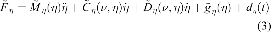
According to the literature, 2,3 the equations of a 6DOF underwater vehicle model in the earth-fixed representation (Figure 1) has the form


where

Frames for 6DOF underwater vehicle. DOF: degree-of-freedom.
Remark. In the method used to decompose the matrix
where the uncertain terms
To obtain the transformed equations of motion, we introduce the vector


where

The determined
Assuming all disturbances vector using equation (3), the new equation of motion is derived in the following way. We take into consideration equation (5) and insert equation (4) into equation (1). Then, both sides of the resulting equation are multiplied by


where the matrices and vectors are given as follows


Equations (7) and (8) are expressed in quasi-velocities and relate to the motion of a 6DOF underwater vehicle. The diagonal matrix

The equations shown above are the basis for applying the proposed strategy of vehicle dynamics model evaluation.
Underwater vehicle dynamics model test scheme
The proposed method consists of two stages: (1) designing of a controller which contains the system parameters set in the gain matrices and (2) dynamics analysis based on a comparison between the selected control algorithm and a reduced controller that does not contain dynamics in these matrices. The second stage, which enables the dynamics study, is realized according to the proposed procedure shown in Figure 2.
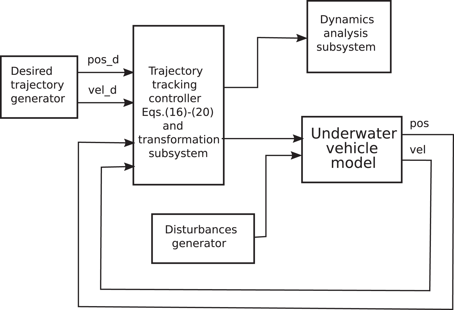
Scheme of the approach.
In block Desired trajectory generator, the desired position and velocity trajectories are generated. Block Disturbances generator is used to generate functions describing all disturbances. In block Underwater vehicle model, the vehicle model is included and the signals in the form of forces and torques are converted into its current positions and velocities. In block Trajectory tracking controller and transformation subsystem, the set positions of the trajectory to be tracked and the set velocities are compared with the current positions and velocities. It also includes the controller and the variable transformation subsystem. The obtained signals are sent to Dynamics analysis subsystem used for their analysis and generation of results.
Controller
In this subsection, the control algorithm and the proposed dynamics analysis scheme are presented.
Assumption 1
(a) It is assumed that the desired trajectories
(b) The uncertainty vectors
(c) The control input vector
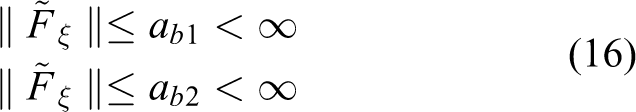
Comment. The problem of the boundedness of the lumped uncertainty vector was considered, for example, in the literature. 13 It was shown that taking into consideration equations (1) to (3), the bound can be described by

where bi (
Assumption 2
The following inequality is assumed

The assumptions were made, for example, in the literature 15,16 and it was applied for underwater vehicle control.
Proposition
We assume the dynamics model (7) and expressions (8) and (4) together with the following control scheme

where


The symbols
Remark. The gain matrices kD, kP,
Proof
The systems (7), (8), and assuming the control algorithm (19) are described as follows

Next, we define the proposed Lyapunov function candidate

Determining the time derivative of the function

Applying equation (9), we calculate
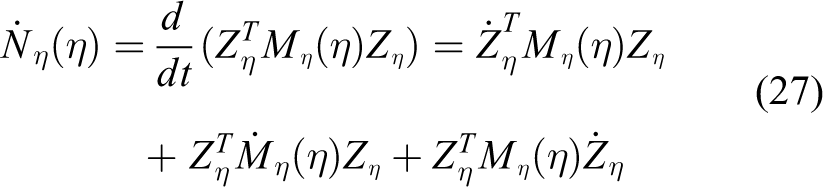
Next, we use equation (24) and insert equations (10) and (27) into equation (26). Taking into account the property

Now, we prove that
But, it is also

Recalling that
As a result, the term in the second line of equation (28) is zero. Moreover, using equation (23), we have the relationships

Note that, if Assumptions 1 and 2 hold, then it can be written as follows

From the literature,
15
it arises that equation (32) does not guarantee that
The function
Remark. For slowly moving vehicles, the vector
Dynamics analysis scheme
The model analysis using the proposed controller is given in several steps.
Step 1. The GVC controller (19) is transformed to obtain the input signals. The signal from the proposed controller (19) is transformed into
Step 2. We compare the results obtained using equation (19) with the performance from the algorithm (called CL), which does not contain the dynamical couplings in the same form (for the same control gains, but without the matrix N and

The symbols mean:
Step 3. Based on results using the GVC and CL controllers, the following time responses are analyzed: (1) the position errors
Step 4. In the vector
Each variable
Step 5. We determine the effect of dynamical coupling on velocities and input signals. Analyzing the time history of quasi-velocities

The quantity
The dynamical couplings are present in the second term. We define the measures of couplings as follows

Step 6. Analysis of the effects of vehicle dynamics and dynamic couplings on the basis of simulation results using GVC and CL controllers.
Simulation results
The goal of the simulations is to verify the proposed approach. The method is suitable both for testing models of known vehicles and those that are just being designed. It means that at the design stage, various models can be examined. The results obtained can then be used to change the design of the vehicle. Moreover, the same decomposition method is applied for the matrices
Main test—vehicle 1
Here, the used vehicle model and its parameters are based on the data from references.
37
The parameters of the vehicle model can be compared with the parameters of real underwater vehicles, for example, Cyclops
38
or a heavier BA-1 vehicle.
39
Due to design limitations, the control inputs were bounded
Steps 1 and 2
The following desired trajectory profiles were selected

The start points were
The disturbance vector, in which all unknown dynamics and other the external disturbances are present, is given by the applied force and torque vector
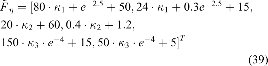
where

For the CL controller,
Remark
The proposed method does not consist of searching for the best gains of the CL control algorithm because it can be done by adopting a different method of selecting gains. The essence of the problem is to find a set of gains for the GVC controller that guarantees acceptable error convergence results because the dynamic parameters of the vehicle are present in the gains. Then, for the CL controller, the matrices of gains without dynamic parameters are adopted, which makes the obtained results different. Based on these differences, the effect of dynamics on vehicle motion is evaluated.
Step 3
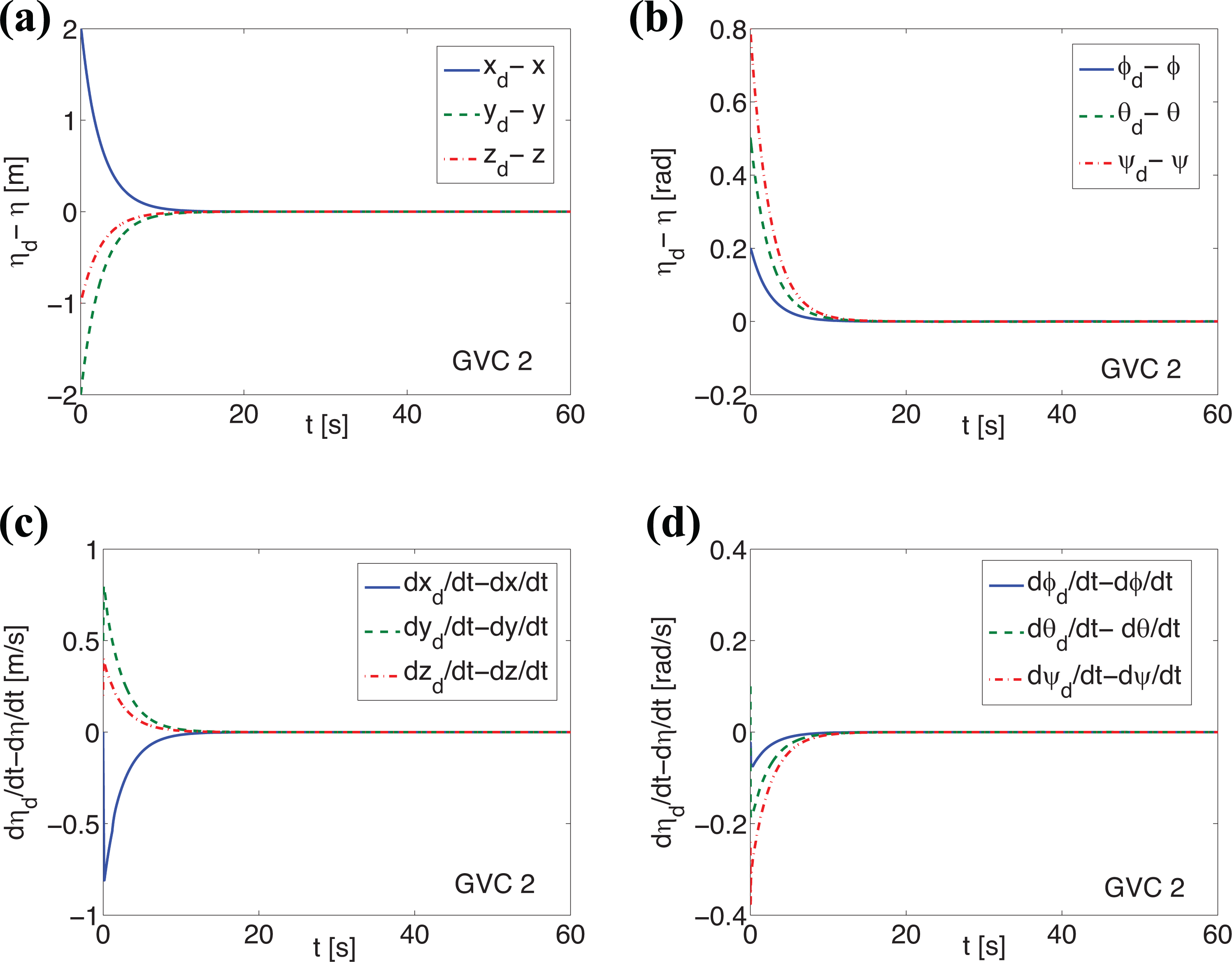
The tracking errors both for position and velocity obtained using the GVC control algorithm are shown in Figure 3. The analogous errors for the CL controller are depicted in Figure 4. From Figure 3(a) and (b), one can see that all errors tend to zero in 10 s. Thus, GVC controller works quickly and correctly. From Figure 4(a) and (b), it is depicted that the CL algorithm is less effective than the GVC one. Moreover, it appears that fluctuation of errors

Response—GVC algorithm (vehicle 1): (a) position errors tracking (linear); (b) position errors tracking (angular); (c) velocity errors tracking (linear); and (d) velocity errors tracking (angular). GVC: generalized velocity component.
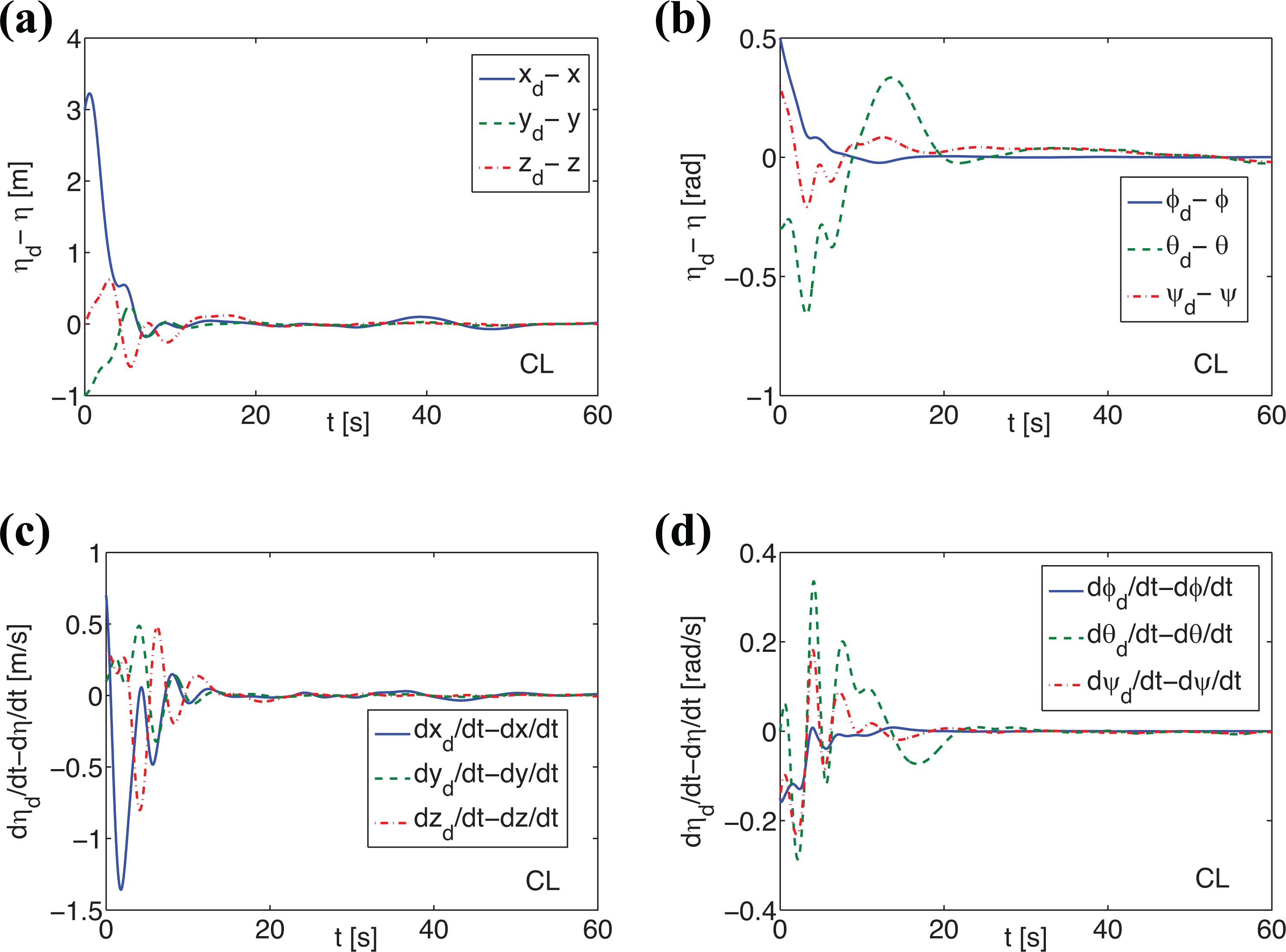
Response—CL algorithm (vehicle 1): (a) position errors tracking (linear); (b) position errors tracking (angular); (c) velocity errors tracking (linear); and (d) velocity errors tracking (angular). CL: classical.
The applied forces and torques in the earth-fixed frame (

Response—GVC algorithm (vehicle 1): (a) applied forces; (b) applied torques; (c) lumped dynamics estimation errors

Response—CL algorithm (vehicle 1): (a) applied forces; (b) applied torques; (c) lumped dynamics estimation errors
Step 4
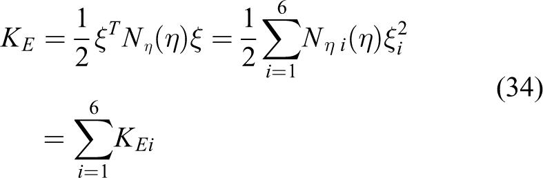
Evaluation of the kinetic energy related to each GVC variable
Step 5
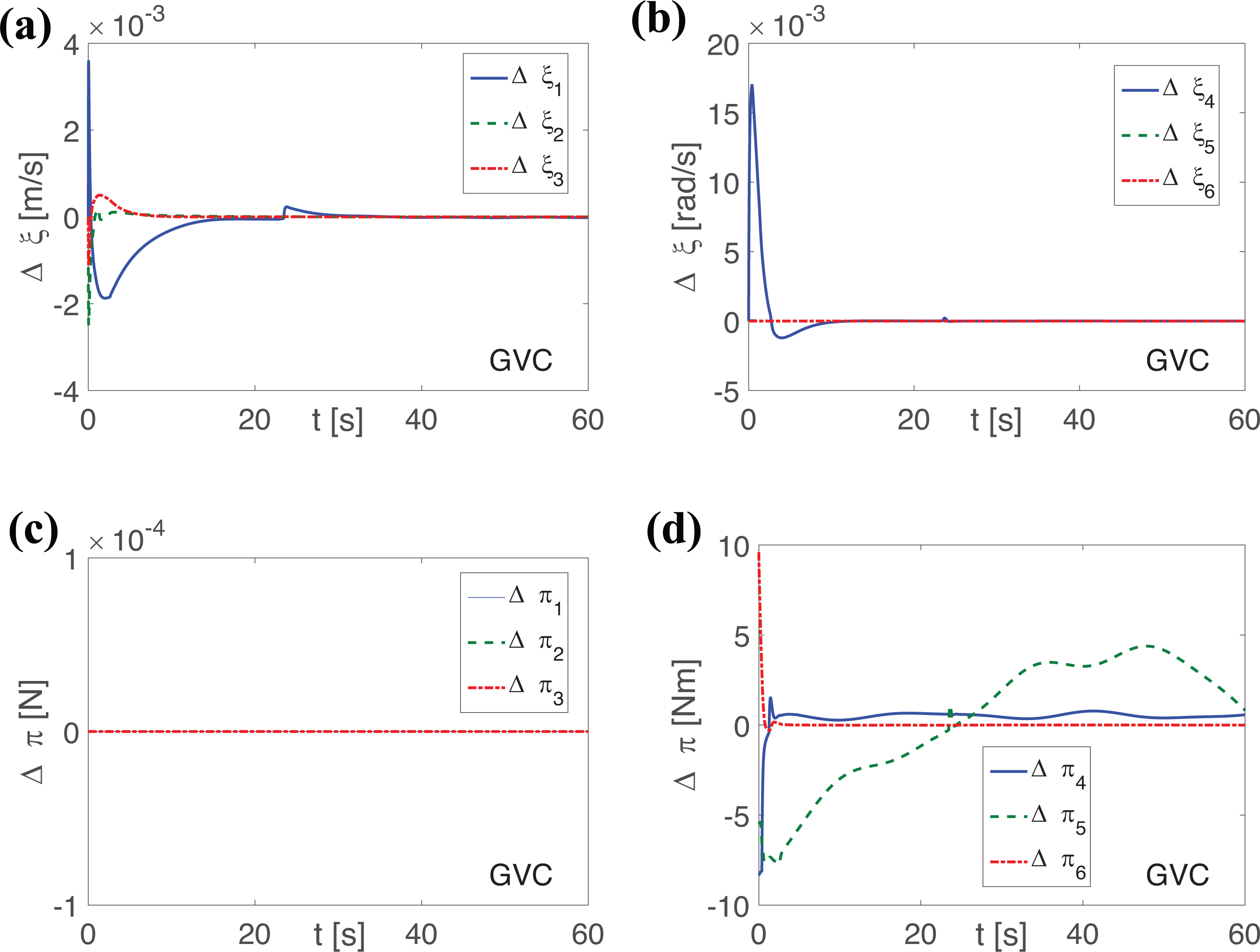
The GVC controller (37) is used to determine the effect of the dynamical couplings. As it is observable from Figure 7(a), the velocity

Response—GVC algorithm (vehicle 1): (a)
Step 6
Finally, the results of the simulation are discussed. The assumed tracking trajectory and the considered model effect of dynamics in the control gains were evaluated on the basis of conducted tests. Comparing the control algorithms GVC and CL, we have found that for the first one, the error convergence is fast. From the time history of errors, it is shown that y, z,
Controller test
To show some of the properties of the proposed control algorithm, two additional tests are performed. In both examples, the same as previously, that is, equation (40) gain set was used.
Example 1
First desired trajectory and second disturbance vector. The desired profiles are described by equation (38), whereas the second disturbance vector was assumed in the form

where

Response—GVC algorithm (vehicle 1) Example 1: (a) position errors tracking (linear); (b) position errors tracking (angular); (c) velocity errors tracking (linear); and (d) velocity errors tracking (angular). GVC: generalized velocity component.
Example 2
Second desired trajectory and second disturbance vector. In this case, the following second desired trajectory profile was used

The start points were
As the working conditions of the controller were changed, the position and velocity errors were also different, as shown in Figure 9. This figure shows that the errors are close to zero after about 15 s, that is, in a slightly longer time than for the first desired trajectory. This is the result of changing the trajectory. Nevertheless, the controller performs the task correctly. Comparing Figure 5(a) and (b) with Figure 10(a) and (b), it can be seen that the changes of applied forces and torques are not very large. However, the lumped dynamics estimation errors associated with the forces are large in a shorter time when the second trajectory (Figure 10(c)) is realized than for the first trajectory (Figure 5(c)). In contrast, the final limits have higher values for the second desired trajectory. From Figure 5(d) and 10(d), it can be observed that the lumped dynamics estimation errors related to the applied torques have greater values when the first desired trajectory is used.
Response—GVC algorithm (vehicle 1) Example 2: (a) position errors tracking (linear); (b) position errors tracking (angular); (c) velocity errors tracking (linear); and (d) velocity errors tracking (angular). GVC: generalized velocity component.

Response—GVC algorithm (vehicle 1) Example 2: (a) applied forces; (b) applied torques; (c) lumped dynamics estimation errors

Response—GVC algorithm (ODIN): (a) position errors tracking (linear); (b) position errors tracking (angular); (c) velocity errors tracking (linear); and (d) velocity errors tracking (angular). GVC: generalized velocity component.
Main test—vehicle 2 (ODIN)
The second tested vehicle was ODIN. Its parameters were assumed from the literature.
35
Due to design limitations, the control inputs were bounded
Steps 1 and 2
The used desired trajectory was defined by equation (38) with initial points
After some trials, the following gain set was selected

For the CL controller,
Step 3
The position and velocity tracking errors for the GVC control algorithm are shown in Figure 11 while for the CL controller in Figure 12. From Figure 11(a) to (d), it can be observed that all errors are close to zero after about 30 s. Such a result proves the correct action of the controller. On the contrary, the results obtained for the CL controller (Figures 12(a) to (d)) show that it is inefficient and does not work properly. As can be seen from Figure 13(a) to (d), the applied forces and torques for both controllers (GVC and CL) have acceptable values and a time history of movement duration.

Response—CL algorithm (ODIN): (a) position errors tracking (linear); (b) position errors tracking (angular); (c) velocity errors tracking (linear); and (d) velocity errors tracking (angular). CL: classical.

Response—ODIN: (a) applied forces (GVC); (b) applied torques (GVC); (c) applied forces (CL); and (d) applied torques (CL). GVC: generalized velocity component; CL: classical.
Step 4
For ODIN, the mean value of the kinetic energy calculated according to equation (34) is
Step 5
The GVC controller (37) is used to determine the dynamical couplings. As can be observed in Figure 13(a) and (b), linear velocity couplings are more than 10 times less than for vehicle 1, but angular velocity couplings have comparable values. The velocities
Response—GVC algorithm (ODIN): (a)
Step 6
For the used tracking trajectory and the ODIN model, effects of dynamics in the control gains were evaluated. The GVC controller, which contained the dynamic parameters of the vehicle in gains, performed the task of tracking the desired trajectory correctly. On the contrary, the CL controller that did not contain the dynamic parameters in the gain matrices failed to perform the same task. The GVC controller gains were selected according to the ODIN vehicle dynamics, but their values proved insufficient to provide acceptable results for the CL controller. The analysis of the dynamics together with the dynamical couplings has shown that deformation of velocities is related to
Discussion of results
In the simulations, the procedure of testing the effects of vehicle dynamics on trajectory tracking was verified. Two models of underwater vehicles with clearly different dynamics and couplings were used for the test. As shown in the literature, dynamic couplings for vehicle 1 37 are significant while for vehicle ODIN 35 are very weak. The advantage of the GVC controller is that its gain matrices contain the vehicle’s dynamic parameters together with the dynamic couplings. As a result, the set of these gains is consistent with the vehicle dynamics and the position and velocity errors are adjusted according to the vehicle dynamics. This allows to obtain sometimes better results than for a classical controller, where even if the gains are selected correctly, they are not directly related to the vehicle dynamics. It turned out that another important advantage of the GVC controller is that it can detect the effect of vehicle dynamics and dynamic couplings when the vehicle is in motion.
Vehicle 1
The quantitative effect of vehicle dynamics on position and velocity errors can be detected based on Figures 3 and 4, while on applied forces and torques from the comparison of Figures 5 and 6. More detailed information about the deformation of velocities and applied forces, and torques was obtained from Figure 7. Because in the case of vehicle 1, the dynamic couplings were significant and the
Vehicle 2—ODIN
The effect of vehicle dynamics and dynamic couplings for this vehicle is observed by comparing Figures 11 and 12. However, it turned out that omitting the vehicle’s dynamic parameters in the CL controller caused it not to work properly and the results were unacceptable. On the contrary, when using the GVC controller, the task of trajectory tracking was done correctly. This phenomenon can be explained by the fact that the gain matrices
Conclusions
A method for simulating the effect of dynamics and dynamical couplings in the gain matrices of a trajectory tracking control algorithm with a disturbance model is presented in this work. The approach is applicable for fully actuated underwater vehicles what means that all input signals are available. It is composed of three tasks: transformation of equations of motion, design of controller in the vehicle external frame, and its use for investigation of the vehicle dynamics. The procedure for the dynamics analysis is given in detail. Simulations conducted on two underwater vehicle models show possible use of the GVC controller (together with CL algorithm) for the dynamics and couplings evaluation. The method is primarily useful for testing the dynamics of the vehicle. The purpose of the test is to provide an insight into the dynamics, the couplings, and consequences arising from the assumption of the vehicle model and the disturbance vector. If the results of the signals are very divergent for the GVC and the CL controller, this means that taking into account the dynamics of the vehicle together with the couplings in the controller’s gains is important for its proper operation. In addition to showing the simulation results obtained for the basic test, the results of tests using a different desired trajectory than in the main test and for a different function describing the disturbances are also presented. In summary, based on the presented control algorithm, it is possible to estimate the effects of the coupling influence on the vehicle motion avoiding an experiment on a real object or at the stage of planning such an experiment. Sometimes, based on simulations, it can be decided whether an experiment is needed (if the results are unacceptable). When such a case occurs, it is necessary to change the model parameters. The obtained results can be next used for experiment planning. In the future, other vehicle models, disturbance models, and trajectories are planned for the dynamics study.
Footnotes
Declaration of conflicting interests
The author(s) declared no potential conflicts of interest with respect to the research, authorship, and/or publication of this article.
Funding
The author(s) disclosed receipt of the following financial support for the research, authorship, and/or publication of this article: This work was supported by Poznan University of Technology under grant no. 09/93/DSPB/0611.