Sage Journals: Discover world-class research

Abstract

The article presents a friction dynamic modeling method for a flexible parallel robot considering the characteristics of nonlinear friction. An approximate friction model which is proposed by Kostic et al. is applied to establish the dynamic model with Lagrange method. Parameters identification is completed by least square method, and the tracking accuracy and the stability of the robot are systematically analyzed before and after dynamic compensation at different speeds. Its position error of the robot after compensation is only 0.98 mm at low speed. The accuracy is improved 10 times than that before compensation. In addition, the peak velocity errors are 3.97 mm·s⁻¹ and 1.49 mm·s⁻¹ at high and low speed, respectively, which are reduced 2.5 times than that before compensation. The experimental data also indicate that velocity tracking curve has no obvious peak error compared with the common method based on Coulomb and viscous friction model. The curve is much smoother with proposed model, and the motion stability of robot at high speed has been greatly improved. The proposed method just needs the robot to collect some positions before path tracing, and the parameters identification of dynamic model can be completed quickly. The compensation effect is much more better than common method. So the proposed method can be extended to complete the dynamic identification for complex robot with more joints. It is helpful to further improve the stability and the accuracy at high speed.

Keywords

Flexible parallel robot nonlinear friction dynamic modeling peak error stability

Introduction

The development of robot technology has great significance in improving the competitiveness of advanced production and promoting the national economy. The serial robot has the characteristics of simple structure and easy operation. It was first used in industrial production.^1

–4 However, it has some problems of error accumulation effect and low load because of single chain structure. The parallel mechanism has the advantages of strong load capacity, large stiffness, and no accumulation of errors.^5,6 But it is difficult to build dynamic model because of multiple chains and a large number of joints.^7,8 At present, kinematic calibration and error compensation are usually used to improve the accuracy of robot. For improving the stability of the mechanism, the research on dynamic parameter identification has important theoretical research engineering.^9

–12 The dynamic model of the parallel robot can describe the relationship between the robot’s motion and the torque of each joint. The stability of the robot’s actual trajectory tracking can be reflected by the friction force curve. It has proved that, the nonlinear friction of the driving joints makes an increasingly prominent impact on the accuracy, motion stability, and rapidity of the robot.¹³ The dynamic modelling methods of parallel robot can be divided into Newton–Euler method and Lagrange method. Compared with Newton–Euler method, the dynamic model which is obtained by Lagrange method is more concise. Therefore, in the field of parallel robot design, Lagrange method has been widely used. For the high-speed parallel mechanism, the inertia load of each linkage is directly proportional to rotating speed of the original component. With the increase of velocity, the effect of joint friction becomes more obvious, and it often results in different degrees of shaking on the trajectory tracking.¹⁴ Therefore, the dynamic identification and compensation to improve the stability of robot system have gradually become a focus of attention.

The friction is the main factor that affects the stability of the robot system. It will cause large steady-state error of the system and a dead zone near zero speed.¹⁵ Therefore, scholars have carried out research on the speed control strategy.^16,17 At present, the main velocity planning algorithm includes ladder velocity control algorithm (LVCA) and S-type velocity control algorithm (SVCA). The latter is named for its S-shaped speed curve, which is widely used in high-speed and high-precision machining systems.^15,18 The SVCA is suitable for 3D trajectory tracking of robot with high stability and accuracy, but it owns many parameters which result the algorithm become more complex.^19,20 The LVCA is relatively simple and easy to be implemented. The accuracy is poorer than SVCA when robot moves on 3D trajectory path. So the LVCA is widely applied in the control of planar industrial robots. The researched robot in the article is mainly used for precise positioning and arbitrary trajectory tracking in the work plane. It is widely used in the industrial field because of its low cost, simple structure, and easy control.

Many scholars have discussed and summarized the friction characteristics and models. Berger²¹ introduced the friction models and typical dynamic response in different fields. Liu et al.²² introduced the friction phenomenon and common friction model in mechanical system, which provided reference for the selection of friction model in the research, and the results have proved that the compensation effect only based on Coulomb friction, Stribeck friction, viscous friction, and static friction model is not good for robot. The main reason is that the above models are difficult to accurately and comprehensively reflect the nonlinear characteristics of friction force under dynamic motion at high speed. Some researchers focus on the influence of Coulomb friction and viscous friction on the motion trajectory. They propose a convex relaxation method to complete the optimal trajectory and feed-forward control, which is applied to solve the nonconvex problem of the manipulator.^13,23 But this method does not consider the effect of Stribeck friction. Some studies only consider the influence of the viscous friction effect on the motion trajectory.²⁴ However, many researchers just consider the influence of Coulomb friction and viscous friction on the trajectory of the robot, which ignores the actual nonlinear distribution of the manipulator during acceleration and deceleration process.^10,11 Kostic et al.²⁵ proposed an approximate nonlinear friction model, which reflects the coupling characteristics of the Coulomb friction, viscous friction, and Stribeck friction. The exponential function is used to reflect the nonlinear friction characteristic of driving joints during acceleration and deceleration, which is verified in the RRR manipulator. The dynamic model of the robot considering nonlinear friction is established with Lagrange method. An approximate exponential friction model is introduced to dynamic model of robot, and the parameter identification of dynamic is completed by least square method (LSM). On this basis, the robot’s dynamic performance has been analyzed deeply before and after compensation. The feasibility and effectiveness of proposed method are verified by experiments.

In this article, a complete and systematic identification process is presented for an industrial parallel robot using an approximate friction model and LSM. The proposed method just needs to collect some positions data. But these sampling position points should be distributed in the whole working space as far as possible, and the sampling accuracy must be ensured when robot is moving on the preset path. So the article recommends to apply single point sampling method. The proposed method can be used to finish dynamic identification work for other robots with more complex structure. The rest of this article is organized as follows. The second section presents the nonlinear friction dynamic modeling method, which includes the robot’s structure, Lagrange modeling principle and the adopted exponential friction model. The third section includes experimental set, sampling method of position, stability analysis, and validation of proposed method. The last section presents the conclusions.

Nonlinear friction dynamic modeling

The structure of parallel robot

The researched robot in this article is produced by Shenzhen GuGao Tech Company in China, which is mainly used for precise positioning and trajectory tracking on the working plane. It owns some advantages of low cost, simple structure, and easy control. Therefore, the robot has been widely used in industrial field.^14,17 A large number of scholars have made much research on the kinematic modeling, structure error calibration, and dynamic modeling about plane parallel robot. But there are few research on the dynamic parameter identification and compensation effect under considering nonlinear friction.

Fu et al.¹³ has demonstrated that friction force of the drive joints is an important factor that affects the robot accuracy and movement stability on continuous path. In order to improve the robot’s tracing accuracy and stability at high speed, the parameters identification method of dynamics is researched deeply and systematically considering nonlinear friction factor. The robot’s structure is shown in Figure 1.

Figure 1.

The flexible parallel robot.

$F_{i} {(x}_{D i} {,y}_{D i})$ (i = 1, 2, 3) means the position of the driving motor which is fixed on the platform in Figure 2, and $G_{i} (x_{B i}, y_{B i})$ (i = 1, 2, 3) is the passive joint’s coordinate. $L_{D i}$ and $L_{B i}$ are respectively the length of driving rod and the passive rod. $O (x_{o}, y_{o})$ represents the robot’s coordinate. $θ_{i} (i = 1, 2, 3)$ and $θ_{B i} (i = 1, 2, 3)$ are called the driving angle and the passive angle, respectively.

Figure 2.

The robot’s coordinate system.

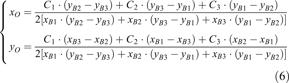
So the coordinate of the robot can be written as

\begin{array}{l} x_{o} = x_{D i} + L_{D i} \cdot cos (θ_{i}) + L_{B i} \cdot cos (θ_{B i}) \\ y_{o} = y_{D i} + L_{D i} \cdot sin (θ_{i}) + L_{B i} \cdot sin (θ_{B i}) (i = 1, 2, 3) \end{array}

with

\begin{array}{l} x_{B i} = x_{D i} + L_{D i} \cdot cos (θ_{i}) \\ y_{B i} = y_{D i} + L_{D i} \cdot sin (θ_{i}) (i = 1, 2, 3) \end{array}

Therefore, the following conclusion is deduced as

{(x_{O} - x_{B i})}^{2} + {(y_{O} - y_{B i})}^{2} = L_{B i}^{2} (i = 1, 2, 3)

Then the equation (3) can be modified as

\begin{array}{l} 2 (x_{B 2} - x_{B 1}) x_{O} + 2 (y_{B 2} - y_{B 1}) y_{O} = C_{2} - C_{1} \\ 2 (x_{B 3} - x_{B 1}) x_{O} + 2 (y_{B 3} - y_{B 1}) y_{O} = C_{3} - C_{1} \end{array}

where $C_{i} (i = 1, 2, 3)$ are defined as

{\begin{matrix} C_{1} = x_{B 1}^{2} + y_{B 1}^{2} - L_{B 1}^{2} \\ C_{2} = x_{B 2}^{2} + y_{B 2}^{2} - L_{B 2}^{2} \\ C_{3} = x_{B 3}^{2} + y_{B 3}^{2} - L_{B 3}^{2} \end{matrix}

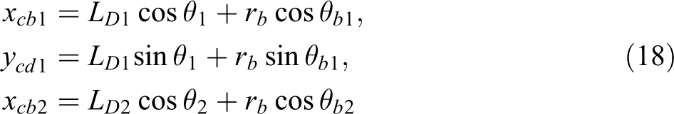
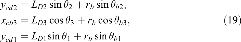
Therefore, the coordinate of robot can be written as

{\begin{matrix} x_{O} = \frac{C_{1} \cdot (y_{B 2} - y_{B 3}) + C_{2} \cdot (y_{B 3} - y_{B 1}) + C_{3} \cdot (y_{B 1} - y_{B 2})}{2 [x_{B 1} \cdot (y_{B 2} - y_{B 3}) + x_{B 2} \cdot (y_{B 3} - y_{B 1}) + x_{B 3} \cdot (y_{B 1} - y_{B 2})]} \\ y_{O} = \frac{C_{1} \cdot (x_{B 3} - x_{B 2}) + C_{2} \cdot (x_{B 1} - x_{B 3}) + C_{3} \cdot (x_{B 2} - x_{B 1})}{2 [x_{B 1} \cdot (y_{B 2} - y_{B 3}) + x_{B 2} \cdot (y_{B 3} - y_{B 1}) + x_{B 3} \cdot (y_{B 1} - y_{B 2})]} \end{matrix}

and the speed of robot is also expressed as

{\begin{matrix} x_{O}' = \frac{C_{1} \cdot (y_{B 2} - y_{B 3}) + C_{2} \cdot (y_{B 3} - y_{B 1}) + C_{3} \cdot (y_{B 1} - y_{B 2})}{2 [x_{B 1} \cdot (y_{B 2} - y_{B 3}) + x_{B 2} \cdot (y_{B 3} - y_{B 1}) + x_{B 3} \cdot (y_{B 1} - y_{B 2})]} \\ y_{O}' = \frac{C_{1} \cdot (x_{B 3} - x_{B 2}) + C_{2} \cdot (x_{B 1} - x_{B 3}) + C_{3} \cdot (x_{B 2} - x_{B 1})}{2 [x_{B 1} \cdot (y_{B 2} - y_{B 3}) + x_{B 2} \cdot (y_{B 3} - y_{B 1}) + x_{B 3} \cdot (y_{B 1} - y_{B 2})]} \end{matrix}

So the velocity $\dot{θ}$ can be written as

{(\begin{matrix} \dot{θ_{1}} & \dot{θ_{2}} & \dot{θ_{3}} & \dot{θ_{B 1}} & \dot{θ_{B 2}} & \dot{θ_{B 3}} \end{matrix})}^{T} = J (\begin{matrix} \dot{x_{o}} \\ \dot{y_{o}} \end{matrix})

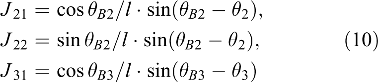
where the matrix J is defined as

J = (\begin{matrix} J_{11} & J_{12} \\ J_{21} & J_{22} \\ J_{31} & J_{32} \\ J_{41} & J_{42} \\ J_{51} & J_{52} \\ J_{61} & J_{62} \end{matrix})

All elements of matrix J are defined as following

J_{21} = cos θ_{B 2} / l \cdot sin (θ_{B 2} - θ_{2}), J_{22} = sin θ_{B 2} / l \cdot sin (θ_{B 2} - θ_{2}), J_{31} = cos θ_{B 3} / l \cdot sin (θ_{B 3} - θ_{3})

J_{32} = sin θ_{B 3} / l \cdot sin (θ_{B 3} - θ_{3}), J_{41} = cos θ_{1} / l \cdot sin (θ_{B 1} - θ_{1}), J_{42} = sin θ_{1} / l \cdot sin (θ_{B 1} - θ_{1})

J_{51} = cos θ_{2} / l \cdot sin (θ_{B 2} - θ_{2}), J_{52} = sin θ_{2} / l \cdot sin (θ_{B 2} - θ_{2}), J_{61} = cos θ_{3} / l \cdot sin (θ_{B 3} - θ_{3})

J_{62} = sin θ_{3} / l \cdot sin (θ_{B 3} - θ_{3})

Lagrange dynamic modeling

The Lagrange function L can be written as⁷

L = T - U

where T represents kinetic energy of system and U denotes the potential energy of system. Because this robot works on the xoy plane, the potential energy U of system will be ignored. The structure of single chain is given in Figure 3. $D_{i} (x_{c d i}, y_{c d i})$ and $B_{i} (x_{c b i}, y_{c b i})$ are respectively gravity center of the driving rod and the passive rod, respectively.

Figure 3.

The structure of single chain.

So, the kinetic energy of the driving rod and the passive rod can be written as

{\begin{matrix} T_{D} = \frac{1}{2} I_{D} {\dot{θ_{}}}^{2} + \frac{1}{2} m_{D} ({\dot{x}}_{c d i} + {\dot{y}}_{c d i}) \\ T_{B} = \frac{1}{2} I_{B} {\dot{θ_{b}}}^{2} + \frac{1}{2} m_{B} ({\dot{x}}_{c b i} + {\dot{y}}_{c b i}) \end{matrix} (i = 1, 2, 3)

where $\dot{θ_{}}$ represents the driving joint’s velocity. I_D and I_B are called moment of inertia. m_D and m_B are the quality of the driving rod and the passive rod, respectively, and $x_{c d i}$ , $y_{c d i}$ , $x_{c b i}$ , and $y_{c b i}$ are defined as

{\begin{matrix} x_{c d i} = r_{d} cos θ_{i} \\ y_{c d i} = r_{d} sin θ_{i} \\ x_{c b i} = L_{D i} cos θ_{i} + r_{b} cos θ_{b i} \\ y_{c b i} = L_{D i} sin θ_{i} + r_{b} sin θ_{b i} \end{matrix} (i = 1, 2, 3)

with

x_{c d 1} = r_{d} cos θ_{1}, y_{c d 1} = r_{d} sin θ_{1}, x_{c d 2} = r_{d} cos θ_{2}, y_{c d 2} = r_{d} sin θ_{2}, x_{c d 3} = r_{d} cos θ_{3}, y_{c d 3} = r_{d} sin θ_{3}

x_{c b 1} = L_{D 1} cos θ_{1} + r_{b} cos θ_{b 1}, y_{c d 1} = L_{D 1} sin θ_{1} + r_{b} sin θ_{b 1}, x_{c b 2} = L_{D 2} cos θ_{2} + r_{b} cos θ_{b 2}

y_{c d 2} = L_{D 2} sin θ_{2} + r_{b} sin θ_{b 2}, x_{c b 3} = L_{D 3} cos θ_{3} + r_{b} cos θ_{b 3}, y_{c d 1} = L_{D 1} sin θ_{1} + r_{b} sin θ_{b 1}

s_{a b 1} = sin (θ_{1} - θ_{b 1}), c_{a b 1} = cos (θ_{1} - θ_{b 1}), s_{a b 2} = sin (θ_{2} - θ_{b 2}), c_{a b 2} = cos (θ_{2} - θ_{b 2})

s_{a b 3} = sin (θ_{3} - θ_{b 3}), c_{a b 3} = cos (θ_{3} - θ_{b 3})

where r_d and r_b represent the length of driving rod and the length of passive rod. Therefore, the Lagrange function of the robot is expressed as

L = \sum_{i = 1}^{3} (\frac{1}{2} ε_{i} {\dot{θ_{i}}}^{2} + \frac{1}{2} μ_{i} {\dot{θ_{b i}}}^{2} + κ_{i} cos (θ_{i} - θ_{b i}) \dot{θ_{i}} \dot{θ_{b i}}) (i = 1, 2, 3)

In which these parameters $ε_{i}$ , $μ_{i}$ , and $κ_{i}$ are defined as

{\begin{matrix} ε_{i} = I_{D i} + m_{D i} r_{d i}^{2} + m_{B i} l^{2} \\ μ_{i} = I_{B i} + m_{B i} r_{b_{i}}^{2} \\ κ_{i} = m_{B i} l r_{b_{i}}^{} \end{matrix}

Then the Lagrange equation can be expressed as

\frac{d}{d t} \frac{\partial L}{\partial \dot{θ}} - \frac{\partial L}{\partial θ} = τ

where $τ$ means the torque of the joints, it is defined as

τ = {[\begin{matrix} τ_{θ_{1}} & τ_{θ_{2}} & τ_{θ_{3}} & τ_{θ_{b 1}} & τ_{θ_{b 2}} & τ_{θ_{b 3}} \end{matrix}]}^{T}

So the dynamic model can be written as

M \ddot{θ} + \dot{M} \dot{θ} - \frac{\partial}{\partial θ} (\frac{1}{2} {\dot{θ}}^{T} M \dot{θ}) + \frac{\partial U}{\partial θ} = τ

The above equation (26) can be simplified as

M \ddot{θ} + C \dot{θ} = τ

In which M and C are defined as following

C = [\begin{matrix} 0 & 0 & 0 & m_{B 1} l r_{b_{1}}^{} s_{a b 1} {\dot{θ}}_{b 1} & 0 & 0 \\ 0 & 0 & 0 & 0 & m_{B 2} l r_{b_{2}}^{} s_{a b 2} {\dot{θ}}_{b 2} & 0 \\ 0 & 0 & 0 & 0 & 0 & m_{B 3} l r_{b_{3}}^{} s_{a b 3} {\dot{θ}}_{b 3} \\ - m_{B 1} l r_{b_{1}}^{} s_{a b 1} {\dot{θ}}_{1} & 0 & 0 & 0 & 0 & 0 \\ 0 & - m_{B 2} l r_{b_{2}}^{} s_{a b 2} {\dot{θ}}_{2} & 0 & 0 & 0 & 0 \\ 0 & 0 & - m_{B 3} l r_{b_{3}}^{} s_{a b 3} {\dot{θ}}_{3} & 0 & 0 & 0 \end{matrix}]

M = [\begin{matrix} I_{D 1} + m_{D 1} r_{d 1}^{2} + m_{B 1} l^{2} & 0 & 0 & 0 & 0 & 0 \\ 0 & I_{D 2} + m_{D 2} r_{d 2}^{2} + m_{B 2} l^{2} & 0 & 0 & 0 & 0 \\ 0 & 0 & I_{D 3} + m_{D 3} r_{d 3}^{2} + m_{B 3} l^{2} & 0 & 0 & 0 \\ m_{B 1} l r_{b_{1}}^{} & 0 & 0 & I_{B 1} + m_{B 1} r_{b_{1}}^{2} & 0 & 0 \\ 0 & m_{B 1} l r_{b_{2}}^{} & 0 & 0 & I_{B 1} + m_{B 1} r_{b_{2}}^{2} & 0 \\ 0 & 0 & m_{B i} l r_{b_{3}}^{} & 0 & 0 & I_{B 3} + m_{B 3} r_{b_{3}}^{2} \end{matrix}]

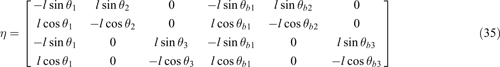
The constraint condition of the researched robot is written as

H (θ) = H {(\begin{matrix} f_{1} (θ) & f_{2} (θ) & ..... & f_{m} (θ) \end{matrix})}^{T} = 0

where the matrix $H (θ)$ is defined as

H (θ) = [\begin{matrix} x_{D 1} + l cos θ_{2} + l cos θ_{b 1} - x_{D 2} - l cos θ_{2} - l cos θ_{b 2} \\ y_{D 1} + l sin θ_{2} + l sin θ_{b 1} - y_{D 2} - l sin θ_{2} - l sin θ_{b 2} \\ x_{D 1} + l cos θ_{2} + l cos θ_{b 1} - x_{D 3} - l cos θ_{3} - l cos θ_{b 3} \\ y_{D 1} + l sin θ_{2} + l sin θ_{b 1} - y_{D 3} - l sin θ_{3} - l sin θ_{b 3} \end{matrix}]

Then the velocity constraint of any point in the workspace can be expressed as

\frac{d H (θ)}{d t} = S (θ) \dot{θ} = 0

In this formula, $S (θ)$ is called the velocity constraint matrix, and the acceleration constraint condition also can be obtained as⁷

\frac{d^{2} H (θ)}{d t^{2}} = S \ddot{θ} + \dot{S} \dot{θ} = 0

Therefore, the dynamic model of system including the velocity constraint can be obtained as

M \ddot{θ} + C \dot{θ} = τ + S^{T} η

where S^T is the velocity constraint matrix, and $η$ is defined as

η = [\begin{matrix} - l sin θ_{1} & l sin θ_{2} & 0 & - l sin θ_{b 1} & l sin θ_{b 2} & 0 \\ l cos θ_{1} & - l cos θ_{2} & 0 & l cos θ_{b 1} & - l cos θ_{b 2} & 0 \\ - l sin θ_{1} & 0 & l sin θ_{3} & - l sin θ_{b 1} & 0 & l sin θ_{b 3} \\ l cos θ_{1} & 0 & - l cos θ_{3} & l cos θ_{b 1} & 0 & - l cos θ_{b 3} \end{matrix}]

Then the dynamic model can be further modified as

M_{s} \ddot{θ} + C_{s} \dot{θ} = τ_{s}

where M_s , C_s , and $τ_{s}$ are defined as

M_{s} = J^{T} M J, C_{s} = J^{T} (M \dot{J} + C J), τ_{s} = J^{T} τ

The equation (36) can be also written as

{(J^{T})}^{+} (M_{s} \ddot{θ} + C_{s} \dot{θ}) = τ

where ${(J^{T})}^{+}$ is the inverse matrix of J^T .

Nonlinear friction modeling

Fu et al. and Yang et al.^13,26 have proved that the friction force of the driving joints is the main factor which affects the robot’s accuracy and stability under continuous path tracing. Therefore, it is very important to establish an accurate nonlinear friction dynamic model. An approximate frictional force model which synthetically considers common friction characteristics such as Coulomb and Stribeck friction has been used to research on dynamic modeling. It is proposed by Hensens and Kosticwhich is defined as¹²

f ({\dot{θ}}_{i}) = k_{v i} \dot{θ_{i}} + \sum_{n = 1}^{2} f_{n i} (1 - \frac{2}{1 + e^{2 m_{n i} \dot{θ_{i}}}}) (i = 1, 2, 3)

where $\dot{θ_{i}^{j}}$ is the i joint’s angular velocity at the j position of path, and $k_{v i}$ represents viscous friction coefficient. $m_{1 i}$ and $m_{2 i}$ are the approximation coefficient for Coulomb and Stribeck friction. $f_{1 i}$ and $f_{2 i}$ represent the Coulomb and the Stribeck friction which are defined as follows

f ({\dot{θ}}_{1}) = k_{v 1} {\dot{θ}}_{1} + f_{11} (1 - \frac{2}{1 + e^{2 m_{1} \dot{θ_{1}}}}) + f_{21} (1 - \frac{2}{1 + e^{2 m_{2} \dot{θ_{1}}}})

f ({\dot{θ}}_{2}) = k_{v 2} {\dot{θ}}_{2} + f_{12} (1 - \frac{2}{1 + e^{2 m_{1} \dot{θ_{2}}}}) + f_{22} (1 - \frac{2}{1 + e^{2 m_{2} \dot{θ_{2}}}})

f ({\dot{θ}}_{3}) = k_{v 3} {\dot{θ}}_{3} + f_{13} (1 - \frac{2}{1 + e^{2 m_{1} \dot{θ_{3}}}}) + f_{23} (1 - \frac{2}{1 + e^{2 m_{2} \dot{θ_{3}}}})

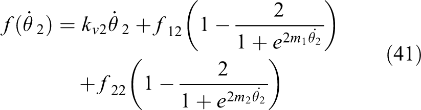
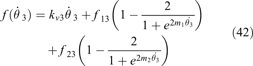
Therefore, the dynamic model considering active joints’ friction can be written as

{(J^{T})}^{+} (M_{s} \ddot{θ} + C_{s} \dot{θ}) + k_{v} \dot{θ} + \sum_{n = 1}^{2} f_{n} (1 - \frac{2}{1 + e^{2 m_{n i} \dot{θ}}}) = τ (i = 1, 2, 3)

Because the input torque of control system is digital, the ratio between the standard unit of torque and the quantitative torque is defined as k_f . The nonlinear friction dynamic model can be expressed as

k_{f} E + k_{v} \dot{θ} + \sum_{n = 1}^{2} f_{n} (1 - \frac{2}{1 + e^{2 m_{n i} \dot{θ}}}) = τ

where E, M_s , and C_s are defined as follows

E = {(J^{T})}^{+} (M_{s} \ddot{θ} + C_{s} \dot{θ}), M_{s} = J^{T} M J, C_{s} = J^{T} C J

Therefore, the optimal function can be written as

f = \sum_{j = 1}^{N} \sum_{i = 1}^{3} (τ_{θ i}^{j} - k_{f} E_{i}^{j} - k_{v i} \dot{θ_{i}^{j}} - f_{1 i} (1 - \frac{2}{1 + e^{2 m_{1 i} \dot{θ_{i}^{j}}}}) + f_{2 i} (1 - \frac{2}{1 + e^{2 m_{2 i} \dot{θ_{i}^{j}}}})) (i = 1, 2, 3)

where $τ_{θ i}^{j}$ and $E_{i}^{j}$ are the i joint’s driving torque and dynamic torque at the j position, respectively. Sixteen parameters such as $k_{v i}$ , $f_{1 i}$ , $f_{2 i}$ , $m_{1 i}$ , $m_{2 i}$ , and k_f (i = 1, 2, 3) will be identified which are dimensionless parameters. We need to calculate the minimum value of optimization function f, and $τ_{θ i}^{j}$ , $E_{i}^{j}$ , and $\dot{θ_{i}^{j}}$ can be obtained from robot system.

We will apply the function of LSM which is provided by MATLAB2016a to complete the optimization calculation based on experimental data. The LSM has some advantages of high efficiency and mature algorithm which are widely used in solving calculation of extremum problem. A set of parameters will be obtained which can make the objective function to be minimum by iterative calculations. The detailed principle can be found in Jorge et al. and Bao et al.^5,27

Experiments

In theory, 16 equations can be calculated by collecting 16 position points, and the identification work can be completed by iterative calculations. However, five redundant equations are added to optimization in order to ensure the effectiveness. Therefore, the robot collects 21 positions data. In general, these sampling positions are distributed in the whole working space. The robot moves on line to complete the above sampling work under LVCA at a speed of 300 mm·s⁻¹.

Identification of dynamic parameters

The single-point sampling style is selected to carry out the experiment. The robot stays 2 s at each point to ensure the reliability and accuracy of data collection. All the sampling positions are shown in Figure 4. The 10 green points are distributed on boundary and 11 red points are close to the center area.

Figure 4.

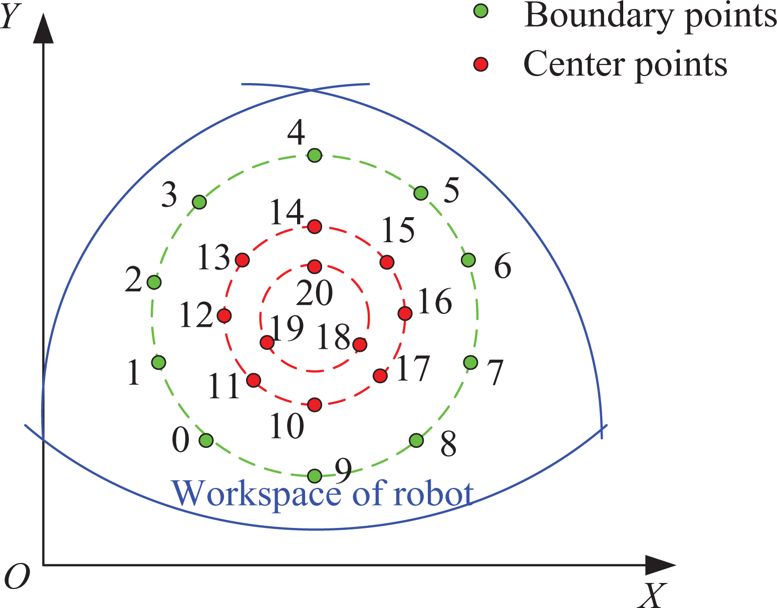
The distribution of sampling points in the workspace.

The robot’s structure parameters are given in Table 1, and the result of identification is shown in Table 2.

Table 1.

Structure parameters of the robot.

Symbols	Joint i
Symbols	1	2	3
Unit	mm	mm	mm
D_i	(0, 200)	( $200 \sqrt{3}, 0$ )	$(200 \sqrt{3}, 400)$
$L_{D i}$	245	245	245
$L_{B i}$	245	245	245

Table 2.

Identification results.

Symbols	Joint i
Symbols	1	2	3
$k_{v i}$	1.632	2.351	0.803
$f_{1 i}$	2.146	−0.702	−1.687
$f_{2 i}$	−0.534	−0.143	0.884
$m_{1 i}$	0.542	−15.610	−0.769
$m_{2 i}$	−17.065	5.368	10.086
k_f	403.712

Table 3.

Coordinates of the start and the end point.

Symbols	Start position E ₁	End postion E ₂
Units	Mm	Mm
x	300	450
y	300	450

The curve of location error curve data can be obtained before and after compensation which is given in Figure 5. It indicates that the position error of the working space boundary (Number 0 to 9) is much larger than the center area. Before compensation, the maximum error is up to 7.09 mm at the boundary area, and it is reduced to 1.88 m after compensation. In addition, the location error in the center area is just ranged from −0.18 mm to 0.19 mm after compensation. Therefore, the nonlinear friction compensation can greatly improve location accuracy in the whole working space. In addition, Figure 5 also indicates that the robot owns better working accuracy in the center area before and after compensation.

Figure 5.

Location error of the robot.

The above data in Figure 5 are further solved and its corresponding histogram including maximum error, average error, and minimum error can be obtained shown in Figure 6.

Figure 6.

Error histogram of robot.

It is not difficult to find that the maximum error of the robot appears in the boundary area. The maximum error before compensation is 7.09 mm, which is reduced to 1.88 mm after compensation. The minimum errors are distributed in the center area which are 0.45 and 0.13 mm, respectively. The average error indicates that the location error is 3.88 mm before compensation. After dynamic compensation, the error is only 0.55 mm which is reduced by an order of magnitude. So the robot’s control accuracy is greatly improved on the whole path.

Experiment setup

In order to verify the effectiveness of proposed method, the robot’s dynamic performance will be tested on the continuous motion. In order to ensure the safety of the robot, it is necessary to define the maximum speed and acceleration of the system when we begin to plan the path. Cai⁷ provides the constraint conditions of the maximum velocity $V_{max}$ and the maximum acceleration $a_{max}$ in workspace W. They are defined as

V_{max} = {min_{θ \in W} \frac{1}{ρ_{max} (J^{+})}} \frac{ω_{max}}{n}, a_{max} = {min_{θ \in W} ρ_{max} (M_{s}^{- 1} J^{T})} n {‖ τ_{θ} ‖}_{max}

where $ρ_{max} (J^{+})$ is the maximum singular value of $J^{+}$ matrix which can be quickly calculated based on dynamic equation by MATLAB, and $ρ_{max} (M_{s}^{- 1} J^{T})$ represents the largest singular value of matrix $M_{s}^{- 1} J^{T}$ . ${‖ τ_{θ} ‖}_{max}$ is the maximum driving torque which can be obtained from motor product manual. n means the reduction ratio, and $ω_{max}$ is called the maximum angular velocity of motor.

n and $ω_{max}$ are considered to be 100 and 3500 r·min⁻¹, respectively. The motion path is set as a line shown in Figure 7, and E ₁ and E ₂ are called the start point and the end point, respectively. The postion coordinates are shown in Table 3. Figure 8 is the control curve of LVCA.

Figure 7.

Motion path of the robot.

Figure 8.

The control curve of LVCA. LVCA: ladder velocity control algorithm.

Table 4 has given the maximum velocity and the maximum acceleration values. In order to ensure the motion security of the robot, actual control parameters are set as 0.40 and 7.00 $m \cdot s^{- 2}$ . The experimental steps are concluded as follows;

Step (1): $E_{1} (x_{q}, y_{q})$ and $E_{2} (x_{e}, y_{e})$ are coordinate of the start point and the end point, respectively. $ϕ$ represents forward angle which can be calculated by $ϕ = a r c t a n (y_{e} - y_{q}, x_{e} - x_{q})$ .

Step (2): $v_{max}$ and $a_{max}^{}$ are given in Table 4, and robot is controlled under LVCA.

Step (3): $s (t)$ is the path function. So the theoretical position at any time can be calculated as follows

{\begin{matrix} x (t) = x_{q} + s (t) cos ϕ \\ y (t) = y_{q} + s (t) sin ϕ \end{matrix}

Step (4): The theoretical velocity and acceleration can be easily obtained at X and Y directions, respectively

{\begin{cases} v_{x} (t) = v (t) cos ϕ, v_{y} (t) = v (t) sin ϕ \\ a_{x} (t) = a (t) cos ϕ, a_{y} (t) = a (t) sin ϕ \end{cases}

Step (5): The sampling time T_c is set 0.001 s, and i is the number of sampling points; the motion time T is quickly calculated with the control parameters. Then the number of sampling points is easy to be computed by $i = T / T_{c}$ .

Step (6): The actual speed of the robot can be obtained by sensors. Then the velocity tracking error at any time is defined as

Δ e_{v (t)} = v (t) - v' (t)

Table 4.

Actual control parameters of robot.

Symbols	$v_{max}$	$a_{max}$
Units	$m \cdot s^{- 1}$	$m \cdot s^{- 2}$
Theory value	0.42	7.10
Actual value	0.40	7.00

Therefore, the angle velocity curve of each driving joint can be obtained based on the above steps.

Figure 9 indicates that when the angular velocity is low, the difference before and after compensation is not obvious about the driving joint 3. It can be seen that the velocity of the joint 3 during uniform stage emerges suddenly changes compared with the other two joints, which is up to 1.81 rad·s⁻¹ without friction compensation shown in Figure 9(a). It also proves that the dynamic performance of the motor is much poorer and friction force seriously affects the stability of the robot’s motion. Figure 9(b) indicates that the stability of all driving joints is greatly improved after compensation. The maximum sudden change of velocity is just 0.58 rad·s⁻¹ which is three times smaller than before compensation. Each joint’s velocity curve on the acceleration stage, the uniform stage, and the deceleration stage are given in Figures 10 to 12, respectively.

Figure 9.

The angular velocity of the three driving joints before and after compensation at speed v = 400 mm·s⁻¹. (a) Before compensation; (b) after compensation.

Figure 10.

Angular velocity of driving joint 1 in different motion stages.

Figure 11.

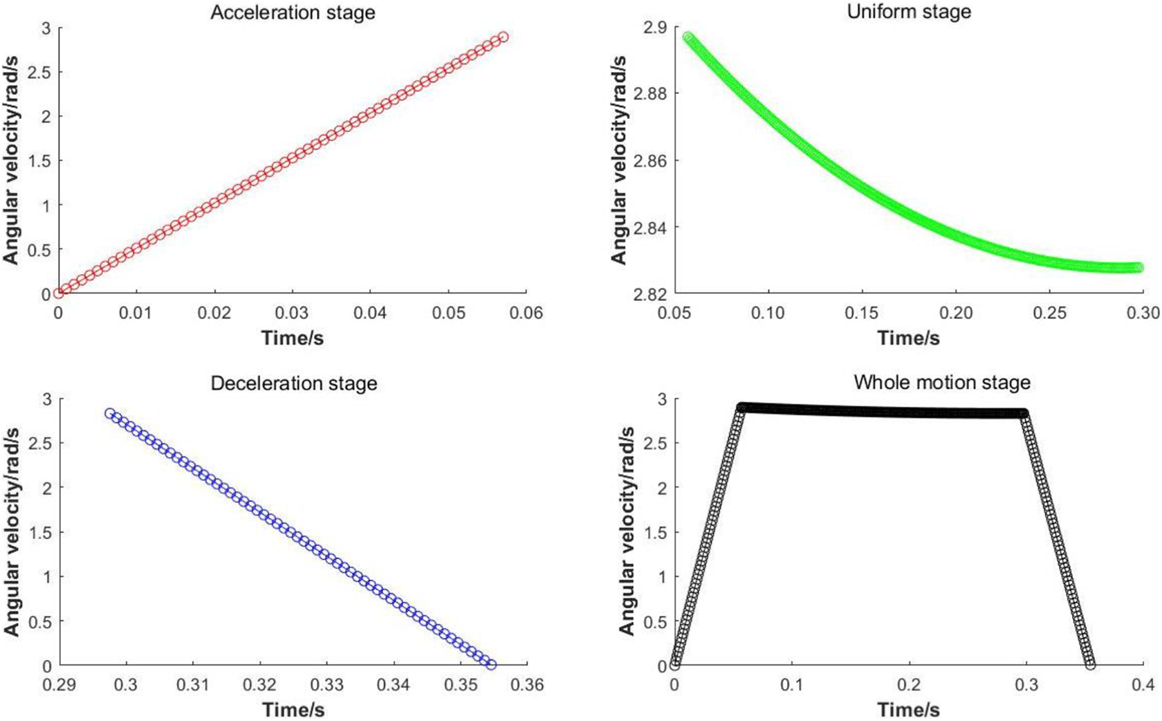
Angular velocity of driving joint 2 in different motion stages.

Figure 12.

Angular velocity of driving joint 3 in different motion stages.

Figure 13.

Nonlinear friction force of driving joints at speed v = 400 mm s⁻¹.

Figures 10 to 12 clearly present that motors can’t work at a constant value in the stage of uniform velocity. The main reason is that nonlinear friction force leads to speed loss in different degrees, and the friction force is closely related to the motor speed. In order to research the coupling mechanism, the nonlinear friction force of each driving joint has been measured. According to the feedback information from speed sensors of driving joints, the friction force curve can be quickly drawn based on the adopted model in this article. Figure 11 indicates that the maximum friction force is distributed in the range of 2.0–7.4 N when the robot is working at uniform stage.

The force variation of driving joint 2 is 0.7 N in the stage of uniform velocity, which is the biggest variation among the three joints. It also demonstrates the stability of driving joint 2 is relatively poorer than other two joints. It shows that nonlinear friction compensation can’t eliminate the influence on the stability of the robot in theory. But accurate model is more helpful to improve the stability by compensation. The maximum value of friction force variation is just 0.7 N at high speed, which indicates the three driving motors work on better condition after compensation. The two exponential functions were applied to the adopted model of friction force to approximate Coulomb and Stribeck friction. The friction force curve of joint 2 shows the characteristics of Coulomb and Stribeck friction are more obvious than viscous friction. It makes the curve appearing exponential distribution in the process of acceleration and deceleration. It can be seen that the friction curve can reflect the characteristic of the speed and the motion stability of the system in different stages. Therefore, in the actual work, the stability of the robot can be quickly analyzed by the velocity tracking performance. Experiment results are given in Figure 13 and Table 5. Figure 13 indicates that the friction force curves of the three driving joints are smooth and the force amplitude is just distributed in the range of 2.2N-7.5N after compensation. It proves the motion stability of robot is good.

Table 5.

The dynamic performance of robot before and after compensation.

v = 400 mm·s⁻¹	Maximum speed peak error	Minimum speed peak error	Average speed error
Before compensation	9.80 mm·s⁻¹	−9.99 mm·s⁻¹	7.76 mm s⁻¹
After compensation	3.97 mm s⁻¹	−3.86 mm s⁻¹	3.43 mm s⁻¹
v = 300 mm s⁻¹	Maximum speed peak error	Minimum speed peak error	Average speed error
Before compensation	7.49 mm s⁻¹	−7.30 mm s⁻¹	4.28 mm s⁻¹
After compensation	2.82 mm s⁻¹	−2.94 mm s⁻¹	2.11 mm s⁻¹
v = 200 mm s⁻¹	Maximum speed peak error	Minimum speed peak error	Average speed error
Before compensation	7.18 mm s⁻¹	−4.92 mm s⁻¹	3.08 mm s⁻¹
After compensation	1.83 mm s⁻¹	−1.92 mm s⁻¹	1.36 mm s⁻¹
v = 100 mm s⁻¹	Maximum speed peak error	Minimum speed peak error	Average speed error
Before compensation	3.98 mm s⁻¹	−3.83 mm s⁻¹	1.94 mm s⁻¹
After compensation	1.49 mm s⁻¹	−1.47 mm s⁻¹	1.32 mm s⁻¹

Table 5 demonstrates that the velocity tracing error becomes greater with the increase of motion speed. When robots work at 400 mm s⁻¹, the maximum and minimum velocity peak errors are 9.80 mm s⁻¹ and −9.99 mm s⁻¹ before compensation, respectively. The data indicate that the stability of the robot is much poorer during acceleration and deceleration process, and its average speed error is up to 7.76 mm s⁻¹. It proves that the tracing accuracy is much poorer than motion on low speed which is consistent with the actual situation. After compensation, the performance of speed tracking is improved obviously. The maximum and minimum velocity peak errors are reduced to 3.97 mm s⁻¹ and −3.86 mm s⁻¹, respectively. It shows that the accuracy and the stability of the motion are greatly improved on the whole path. In addition, when the robot’s speed is closer to the maximum speed limit of 0.42 m s⁻¹, the stability and accuracy become much poorer before and after compensation.

The experimental data have proved that the peak speed error and the average speed error reduce obviously with the speed decreases. The performance of velocity tracing is the best when robot works at 100 mm s⁻¹ based on the four-group experimental data. The maximum speed peak error and the average speed error are 3.98 and 1.94 mm s⁻¹ before compensation, which become to be 1.49 and 1.32 mm s⁻¹ after compensation. The above results also indicate that when the speed is lower, the dynamic compensation effect is not obvious before and after compensation. Its average error difference is only 0.17 mm s⁻¹ before and after compensation. In order to further improve the position accuracy of the robot, kinematic compensation is needed to be completed to further improve accuracy.

Compensation validation

In order to verify the effectiveness of dynamic compensation, we make an experiment to analyze the tracing performance compared with the common friction model. Coulomb and viscous friction force model can be expressed as

f (v) = k_{v} v + s g n (v) \cdot f_{c}

where k_v , v, and f_c are viscosity coefficient, velocity of motor, and Coulomb friction force, respectively. $sgn (v)$ is defined as²²

sgn (v) \cdot f_{c} = {\begin{matrix} f_{c} & v > 0 \\ 0 & v = 0 \\ - f_{c} & v < 0 \end{matrix}

Then the velocity tracing error of the robot is tested before and after compensation at different speeds. Figure 14 indicates that the velocity curve has many peaks and tracing error become larger with the speed increase before compensation. The motion stability of the robot is much poorer at high and low speed because of nonlinear friction force.

Figure 14.

The velocity curve of robot at different speeds.

The smoothness of velocity curve and the tracking accuracy are lower than proposed method in this article at high speed based on Coulomb and viscous model. It is difficult to accurately reflect the nonlinear friction characteristics at high speed based on the linear friction model. The adopted approximate model includes viscous friction and uses two exponential functions to approximate the Coulomb friction and the Stribeck friction. It can truly express the robot’s dynamic characteristics of nonlinear friction at high speed. Therefore, the velocity tracing accuracy and stability are much better than the common method.

Conclusions

In this article, an approximate exponential friction model is applied to establish the nonlinear friction dynamic model for a planar parallel robot. The work of dynamic identification can be completed with LSM just by measuring some position data. The maximum position error is 1.88 mm, which is seven times lower than that before compensation. The average error after compensation is only 0.55 mm, which is reduced an order of magnitude than that before compensation. So friction compensation can improve the location accuracy. Four-group experiments on continuous trajectory tracking have proved that the speed tracking accuracy and stability of the robot at high speed are worse than that at low speed. Before compensation, the velocity curve obviously has many peaks at high speed. Its maximum speed peak error is up to 9.8 mm s⁻¹, and the average error is 7.76 mm s⁻¹. It indicates the motion stability is much poorer in the process of acceleration and deceleration transition. After compensation, the maximum error and average error are reduced to 3.97 and 3.43 mm s⁻¹, and the velocity curve is more smoother, which shows that robot’s stability and the tracing performance are greatly improved, and the friction force curve also confirms this conclusion. The average speed error is 1.94 and 1.32 mm s⁻¹, respectively, before and after compensation when robot works at a low speed of 100 mm s⁻¹. The effect of dynamic compensation is not obvious. Although the stability and velocity tracking accuracy are obviously better than that at high speed, the rapidity of competing tracking is also reduced. The velocity curve of the robot is obviously smoother than that based on Coulomb and viscous model. The results also prove that the adopted friction model in the article can be more realistic to reflect the characteristics of nonlinear dynamic friction. According to the velocity curve, the overall velocity tracing accuracy of the robot is also higher than that at low speed. Therefore, the proposed dynamic compensation method can be extended to improve the stability and tracking performance for other type of robots.

Footnotes

Declaration of conflicting interests

The author(s) declared no potential conflicts of interest with respect to the research, authorship, and/or publication of this article.

Funding

The author(s) disclosed receipt of the following financial support for the research, authorship, and/or publication of this article: This work was supported by National Key Research & Development Program of China [Grant number: 2017YFB1303502], National Natural Science Foundation of China [Grant number: 51975412], and Tianjin Natural Science Foundation of China [Grant number: 18JCYBJC87900].

ORCID iD

Lei Zhao

References

Chen

. Control technology of robot. Beijing: China Machine Press, 2018.

Meng

Zhuang

. Autonomous robot calibration using vision technology. Robot Comput Integr Manuf 2007; 23(4): 436–446.

Chen

Qiu

. The calibration and error compensation techniques for an Articulated Arm CMM with two parallel rotational axes. Measurement 2013; 46(1): 603–609.

Lan

Shiju

. Technology and application of industrial robot. Beijing: Tsinghua University Press, 2019.

Jorge

Juan-Jos

Jos

. Kinematic parameter estimation technique for calibration and repeatability improvement of articulated arm coordinate measuring machine. Precis Eng 2008; 32(4): 251–268.

Klimchik

Caro

, et al. Geometric calibration of industrial robots using enhanced partial pose measurements and design of experiments. Robot Comput Integr Manuf 2015; 35: 151–168.

Cai

. Robotics. Beijing: Tsinghua University Press, 2000.

Han

. Industrial robot. Wuhan: Huazhong University of Science and Technology Press, 2018.

Yamamoto

Trimble

. An experimentally validated analytical model for the coupled electromechanical dynamics of linear vibration energy harvesting systems. J Intell Mater Syst Struct 2017; 28(1): 3–22.

10.

Grotjahn

Heimann

Abdellatif

. Identification of friction and rigid-body dynamics of parallel kinematic structures for model-based control. Multibody Syst Dyn 2004; 11(3): 273–294.

11.

Shang

Cong

Zhang

. Nonlinear friction compensation of a 2-DOF planar parallel manipulator. Mechatronics 2008; 18(7): 340–346.

12.

Hellsen

RHA

Angelis

Van de Molengraft

MJG

, et al. Grey-box modeling of friction: an experimental case-study. Eur J Control 2000; 6(3): 258–267.

13.

Zhan

Huang

. Modeling and compensation of non-linear friction for spatial robotic arm joint. J Mech Trans 2014; 12: 28–32.

14.

Sun

Lin

. A look-ahead path planning algorithm with high speed and high precision. J Mech Eng 2016; 52(11): 170–176.

15.

Liu

Baoyin

. Optimal path planning of redundant free-floating revolute-jointed space manipulators with seven links. Multibody Syst Dyn 2013; 29(1): 41–56.

16.

Kovacs

Szayer

Tajti

. A novel potential field method for path planning of mobile robots by adapting animal motion attributes. Rob Auton Syst 2016; 8(82): 24–34.

17.

Shang

Feng

, et al. Research of trajectory planning for articulated industrial robot. Comput Eng Appl 2018; 54(5): 36–50.

18.

Wang

, et al. Trajectory planning for manipulator in Cartesian space based on constrained S-curve velocity. CAAI Trans Intell Syst 2019; 14(4): 655–661.

19.

Shi

Sun

. B-spline curve algorithm research based on new S velocity planning. Mach Tool Hydr 2016; 44(15): 72–79.

20.

Zhang

Wang

. Research on the algorithm of NURBS curve reverse correction interpolation with S-type acceleration and deceleration control. NC Technol 2019; 9: 162–167.

21.

Berger

. Friction modeling for dynamic system simulation. Appl Mech Rev 2002; 55(6): 535–577.

22.

Liu

, et al. An overview of friction models in mechanical systems. Adv Mech 2008; 38(2): 201–213.

23.

Reynoso-Mora

Chen

Tomizuka

. A convex relaxation for the time-optimal trajectory planning of robotic manipulators along predetermined geometric paths. Optim Control Appl Methods 2016; 37(6): 1263–1281.

24.

Cheng

Yiu

. Dynamics and control of redundantly actuated parallel manipulators. IEEE ASME Trans Mechatron 2003; 8(4): 483–491.

25.

Kostic

Hensen

De Jager

. Modeling and identification of an RRR-robot. In: IEEE 40th conference on decision and control, vol. 2, Orlando, USA, 4–7 December 2001, pp. 1144–1149.

26.

Yang

Shi

. Research on S type acceleration and deceleration time planning algorithm with beginning and end speed non-zero. J Mech Eng 2016; 52(23): 199–206.

27.

Bao

Yang

. Intelligent optimization algorithm and MATLAB example. Beijing: Publishing House of Electronics Industry, 2016.

Nonlinear friction dynamic modeling and performance analysis of flexible parallel robot

Abstract

Keywords

Introduction

Nonlinear friction dynamic modeling

The structure of parallel robot

Lagrange dynamic modeling

Nonlinear friction modeling

Experiments

Identification of dynamic parameters

Experiment setup

Compensation validation

Conclusions

Footnotes

Declaration of conflicting interests

Funding

ORCID iD

References