A review of algorithms and techniques for image-based recognition and inference in mobile robotic systems

Abstract

Autonomous vehicles include driverless, self-driving and robotic cars, and other platforms capable of sensing and interacting with its environment and navigating without human help. On the other hand, semiautonomous vehicles achieve partial realization of autonomy with human intervention, for example, in driver-assisted vehicles. Autonomous vehicles first interact with their surrounding using mounted sensors. Typically, visual sensors are used to acquire images, and computer vision techniques, signal processing, machine learning, and other techniques are applied to acquire, process, and extract information. The control subsystem interprets sensory information to identify appropriate navigation path to its destination and action plan to carry out tasks. Feedbacks are also elicited from the environment to improve upon its behavior. To increase sensing accuracy, autonomous vehicles are equipped with many sensors [light detection and ranging (LiDARs), infrared, sonar, inertial measurement units, etc.], as well as communication subsystem. Autonomous vehicles face several challenges such as unknown environments, blind spots (unseen views), non-line-of-sight scenarios, poor performance of sensors due to weather conditions, sensor errors, false alarms, limited energy, limited computational resources, algorithmic complexity, human–machine communications, size, and weight constraints. To tackle these problems, several algorithmic approaches have been implemented covering design of sensors, processing, control, and navigation. The review seeks to provide up-to-date information on the requirements, algorithms, and main challenges in the use of machine vision–based techniques for navigation and control in autonomous vehicles. An application using land-based vehicle as an Internet of Thing-enabled platform for pedestrian detection and tracking is also presented.

Introduction

Visual sensors include infrared, visible light, laser, millimeter wave, radar, and LiDAR depending on the imaging modality and the environment. They continuously acquire sensory data to model visual scene as an aid in navigation tasks, 2D and 3D scene reconstruction, object and obstacle detection, tracking, recognition, control, and inference. Several functionalities are required for autonomous navigation such as environmental mapping/scene interpretation, path planning, obstacle detection and avoidance, positioning and direction finding, and attention focusing. The availability of technology with 3D scene capture cameras like Microsoft kinect and time-of-flight (TOF) sensors which estimate depth besides measuring scene luminance has significantly increased the spatial, temporal, and spectral details, at the same time increasing the sampling rate, and the processing power requirements. Capturing directly the 3D space of a scene is the future of many areas like scientific research, engineering, virtual reality, augmented reality, and so on. These require special techniques in signal processing such as spectrum estimation, sparse signal processing, and system identification techniques. Event-based cameras, ¹ a biologically inspired visual sensor, present a new paradigm on the way dynamic visual information is acquired and processed. Majority of depth estimation techniques tackle the 3D reconstruction problem using two or more cameras that are rigidly fixed and share a common clock. They first solve the correspondence problem across planes and then triangulate the location of the 3D point. With event-based cameras, visual information is no longer acquired based on external clock (global shutter); instead, each pixel has its own sampling rate based on visual inputs and transmits information about brightness changes of given size (events) only. Clearly, to reconstruct 2D and 3D scenes with high fidelity and to carry out inference and recognition, the problems of high sampling rates and real-time performance must be contended with. ² Innovative signal processing, machine learning, and pattern recognition techniques have been deployed to meet these challenges in a joint image acquisition-processing space. Localization and position verification techniques are also vital in navigation. Traditional approaches use inertial sensing and global positioning system (GPS). The former suffers from the problem of sensor inaccuracies, measurement drifts over time, and requires accurate knowledge of the initial position of the system (autonomous vehicles (AVs)). GPS signals might also not be available, as in indoor environments (office buildings). For radio-based approaches using received signal strength and ranging, the problems of “holes” due to inadequate coverage of all possible configurations must be contended. Adaptive techniques such as neural networks and machine learning have proven capable of adapting very well under such conditions.

The survey focuses on three main types of vision-based navigation in robotics, namely, map-based, maples-based, and map-building-based approaches. ^3,4 Learning-based approaches which train end-to-end systems on robotic tasks (object recognition and manipulation, path planning, obstacle avoidance, etc.) are surveyed, as well as signal processing, machine learning, and evolutionary algorithms. For each algorithmic approach, an introduction to the main algorithm is presented, as well as some details of reported implementations in the literature. The review is general as opposed to detailed review based on a specific approach (e.g. deep learning, optimization-based, and signal-processing-based) since the coverage of the application is wide. Classical robotic navigation algorithms are well presented by Desouza and Kak. ⁴

Sensor representation and perception process

A robot usually creates a model of the environment by acquiring sensory data. Perception is a task-oriented interpretation of sensory data across space and time. It facilitates planning during task execution, controlling the robot itself and its interactions with other robots, and the environment. There are two main types of perception, namely, proprioception and exteroception. The former applies sensing and estimation to recover the state of the robot itself, while the latter estimates the state of the environment. Appropriate sensing and estimation for a given tasks is highly task-dependent. One way of capturing the environment is to construct environmental maps. Maps are defined by the measurements and the location where the measurements have been acquired. They can be parameterized either as a set of spatially located landmarks, dense representation (occupancy maps, and surface maps, or raw sensor representation). The main challenges in creating a model of the environment are incomplete information and the dynamic nature of the environment. Sensing process also suffers from sensing errors, random noise, incomplete measurements, missing data, inadequate dynamic range coverage, and measurement ambiguities. Typical models for the environment may be biologically inspired, ⁶ mathematical, or artificial intelligence based. ⁷ The role of preprocessing is to reduce noise and enhance relevant aspect of the data. In some cases, sensory data might have to be aligned for subsequent integration when data are coming from different sensors.

For optoelectronic signals, sources of noise include sunlight, electrical, and magnetically induced interference and interference from electronic components. Optical filters are normally used to attenuate undesired wavelength, and analogue filters to remove electrical noise. ⁸ Measurement in real environments is also affected by accuracy and precision of the optical scanning system. Flores-Fuentes et al. ⁸ also presented experimental evaluation of different photosensors and their suitability in different operating environments. For indoor positioning or localization without any GPS support, several approaches exist including use of wireless sensors networks, ⁹ cameras and inertial sensors, stereo imaging, and LiDAR. In the context of visible light communication, Rahanjaona et al. ¹⁰ presented an optical sensing device capable of estimating position at a distance of 2 m with an accuracy of 2 cm at a frequency of 100 Hz. To improve the accuracy of spatial coordinate measurements using photodiode and CCD sensors, Flores-Fuentes et al. ¹¹ applied sensor fusion and support vector machine (SVM) regression to predict measurement, lower measurement error probability, and to learn its nonlinear behavior. A technical vision system for mobile robot vision system for industrial robotic application is presented ¹² using a hardware approach, which uses continuous laser scanning and dynamic triangulation for 3D spatial coordinates measurements and control of robots. The system avoids dead zone problem in laser field of view and improves measurement accuracy using servomotor and microcontroller.

An intelligent data acquisition process driven by the measured and partially interpreted scene parameters and errors from the scene has the advantage of making ill-posed perception task tractable. Ferreira et al. ¹³ presented a real-time Bayesian framework for artificial perception of 3D structure and motion using Bayesian volumetric map on CUDA platform. The multimodal perception model combined stereovision, binaural, and inertial sensing to build a model of occupancy and local motion. The map is used to determine gaze shift during active vision exploration. A processing pipeline involving perception typically consists of sensing, preprocessing, feature extraction, data association, parameter estimation, and model update. A network of multiple sensors is beneficial in situations where the sensors cannot provide seamless coverage of the entire region. Considering that multiple sensors may be spatially distributed and watch over objects in different orientations, sensed information has to be aligned via registration. Registration transforms signals to a common reference and typically is achieved by warping or point correspondence. For example, multiview stereo with traditional cameras addresses the problem of 3D structure estimation from a collection of images taken from known viewpoints of an intrinsically calibrated camera by point correspondence. Feature extraction refers to the process of deriving unique characteristics from sensor data for decision-making. It could be mapping of measurements by statistical methods, signal processing, or pattern recognition techniques to features or targets (object of interest). The outcome of the mapping is a measurement event. Data association refers to the process that assigns data measurements by different sensors to targets based on proximity between the sensor measurements. In a multisensor scenario, data association can occur in different processes ^14,15 such as measurement to feature, measurement-to-measurement, and feature-to-feature associations. Conventional data association are based on nearest neighbors or probabilistic association. Data association ¹⁶ can be formulated as a matrix of the form defined by equation (1) (i, k, and t denote measurement, time, and target index, respectively)

$\begin{array}{l}{\mu }^k(t,i)=\{\begin{array}{ll}0& \text{if measurment }i\text{ originated from target }t\\ 1& \text{otherwise}\end{array}\end{array}$

1

Let p(Y^k , ${\mu }^k|X^k$ ) denote the conditional probability of joint measurement event Y^k and data association matrix μ^k , given the state X^k . Then p(Y^k , ${\mu }^k|X^k$ ) = p( $Y^k|X^k$ , μ^k ) p( ${\mu }^k|X^k$ ), Through maximizing the conditional probability, the association matrix can be obtained as

${\mu }^k=\underset{{\mu }^k}{{\displaystyle \text{argmax}}}[\text{log}\hspace{0.17em}p(Y^k|X^k,{\mu }^k)+\text{log}\hspace{0.17em}p({\mu }^k|X^k)]$

2

$X_i^k$ denotes the state (location and pose of a target) associated with measurement i at time k, and X^k denotes all associated measurement state. Y^k similarly denotes all measurement assignment event at time k. The state of a system contains all relevant information required to describe the system. Other uncertainty measures for data association have been investigated using multiple track hypotheses filter. These measurements are applied to mainly address two issues: conflict information, avoid developing different models for different type of sensors, and to develop a more efficient approach for the assignment problem which is NP-hard. ^17,18 For example, fuzzy data association of position and velocity estimates from multiple sensors can be applied to the error covariance based on the current and past measurements. ¹⁶ Data fusion (combining data from multiple sensors) can be carried out at three different levels, namely measurement, track/feature, and decision fusion. Measurement fusion is applied in a centralized process, while distributed sensing usually employs fusion at the feature and decision levels. Decision fusion has been investigated using neural networks, fuzzy logic, ¹⁹ statistical estimation via convex optimization, and stochastic swarm ²⁰ within multiagent frame work, as well as game theory. ^21,22 The problem can be solved by maximizing the likelihood of the joint distribution of the local estimation errors or maximizing the posterior of the conditional mean of the fused feature given the local features. The covariance intersection method ²³ also addressed the potential presence of an unknown correlation in the sensor information. Based on the observation that the fused covariance always lies with the intersection of the two sensor covariance ellipses for all values of the cross correlation. The covariance P_xx of the fused estimate and fused state $X_t^k$ are determined, respectively, by equations (3) and (4)

$P_{xx}^{-1}=w{P}_{ii}^{-1}+(1-w)P_{jj}^{-1}$

3

$X_t^k=P_{xx}\left[w{P}_{ii}^{-1}{X}_{it}^k+(1-w)P_{jj}^{-1}{X}_{jt}^k\right]$

4

The above formulation ensures the optimum weight, w is unique within the range [0 1]. There are numerous techniques that treat jointly the registration, association, and fusion of sensor data. These use extended and unscented Kalman filter (UKF) to estimate states of the augmented systems. ²⁴

Algorithms

Mobile robots are expected to navigate successfully in complex environments, locate and track objects, avoid obstacles, determine their own location, and to reconstruct 3D visual scenes of their environment from cameras and other sensors. Additionally, they may be expected to carry out services to aid humans and industrial inspection. Typically, a service robot might be expected to perform search and rescue, act as human assistance in caring for the elderly by monitoring, and providing timely information about their activities. The rising interest in the use of unmanned aerial vehicles (UAVs) and vision-assisted driving are other scenarios. Traditionally, vision-based systems use stereovision or multiview coding to provide these functionalities. Tracking is typically accomplished using tracking filters ¹⁴ such as Kalman filter, probabilistic data association filter, and multiple sensors fusion and state estimation. For indoor localization and navigational tasks with no external reference support like GPS or wireless location support, simultaneous localization and mapping (SLAM) provides a means of creating an environmental map identifying important obstacles, 3D surface reconstruction, and provides a means of navigating and understanding the external world. Rebecq et al. ¹ presented an algorithm for 3D surface reconstruction from a set of known viewpoints using event-based camera in real time. Although visual inertial/odometry (VI/VIO) uses cameras and inertial measurement units (IMUs) to estimate the state (position, orientation, and velocity) of a robot, it is also able to provide robust state estimation for other tasks such as control, obstacle detection and avoidance, and path planning. For a detailed review of SLAM, Desouza and Kak ⁴ and Cadena et al. ³ are good sources.

Stereo and multiview coding

A stereovision system typically consists of two or more camera systems, each consisting of left and right hand side camera viewing a scene. Each camera pair is calibrated such that its intrinsic and extrinsic parameters are known. To reconstruct a 3D scene of the real world obtained from the two 2D images, the following are the sequence of steps: localization of features in an image; identification and localization of the same features in the other image; and 3D scene reconstruction. Bertozzi and Broggi ²⁵ implemented a vision-based lane detection in driver-assisted vehicle system using monocular stereovision. Multiview stereo with traditional cameras addresses the problem of 3D structure estimation from a collection of images taken from known viewpoints of intrinsically calibrated cameras. One of the limitations of the traditional approach is that only part of the images (features) is used in reconstructing the scene, hence sub optimal, and depth information is inferred. Visual odometry (VO) is used to determine camera’s motion and pose and provides a means for robots to navigate and control in environments where there are no external reference system (e.g. GPS), and the robot must navigate locally. Improved accuracy is achieved by making use of both intensity and depth information. ¹⁹ Traditional approach tracks features in monocular or stereo images and estimates camera’s motion or computes optical flow via feature tracking. ²⁵ To increase precision, features are tracked over several frames (SLAM) opposed as structure from motion problem. With the advent of availability of RGB-D cameras and other depth-based image acquisition sensors like event-based cameras, the trend is now shifting toward computational imaging using low powered devices with small footprints. There are three main camera types, namely depth cameras, stereo and TOF, and light field. The combination of low weight, high dynamic range, low latency, and power consumption makes them suitable for embedded real-time vision applications in mobile platforms. In Rebecq et al., ¹ the camera motion is computed by aligning two consecutive RGB-D images. Instead of aligning images, one can also align 3D point cloud. Iterative closest point (ICP) algorithm ²⁶ is typically applied with its associated high computational cost. Kock ²⁷ showed that given a textured 3D model, the camera pose can be estimated efficiently by minimizing a photometric error between the observed and synthesized model. Recent works indicate that the accuracy of dense alignment can be improved by matching the current image against a model. Examples of such approach include KinectFusion ²⁸ and dense tracking and mapping. ²⁹ Tracking filters are used within the framework of state-space estimation underlying model assumptions to simplify and approximate the state of the system for model parameters estimation and inference. The scenario typically occurs in feature tracking and state estimation problems. Several other problems in computer vision and control can be analyzed assuming a deterministic model of the system or via Bayesian approach.

Visual SLAM

Odometry is the use of data from motion sensors to estimate change in position over time. It is sensitive to errors due to integration of velocity measurement over time. Rapid and accurate data collection, sensor calibration, and near-real-time processing are required to give accurate estimation. VO is an important modality for robot control and navigation in environment when no external position reference such as GPS is available or a prior unknown environments, for example, quadcopters (drone) operating in cluttered indoor environments. VO typically tracks features in monocular or stereovision images and estimates the camera motion between frames. When features are tracked over time, it leads to either SLAM or structure from motion problem, a classical computer vision problem. Bundle adjustment is applied to estimate the pose. ³⁰ A moving robot explores its environment and uses its sensor information to build a “map” of landmarks. Maps can be parameterized as a set of spatially localized landmarks by dense representation like occupancy grids, surface maps, or by raw sensor measurements. The problem of acquiring models of the environment is complex and difficult to solve due to practical limitations on the robots’ ability to learn. The problem stems from the inherent limitations due to sensors and the environment being modelled. Map-based navigation requires high-level process of recognition and analysis to interpret the map and establish its correspondence with the real world. In robotic SLAM, a robot is controlled by a series of inputs that control its movement subject to visual interpretation of the environment, and at the same time building or updating a map. The main sensors used are moving cameras and IMUs. The cameras project 3D points in real-world coordinates to 2D points in image space, and optionally depth image when RGB-depth cameras are used. The pixel coordinates of the tracked features are used as measurements. The IMUs output the angular velocity and the specific force acceleration together with gravity. ^30,31 To facilitate detailed 3D scene reconstruction and understanding modern approaches, use depth cameras or range sensors. Depth provides additional valuable cue for vision tasks such as object localization and scene understanding. The camera configuration is typically in stereo or multiview mode. The main processing steps are image alignment, camera motion estimation, image registration, camera pose tracking, and object/scene segmentation. Traditional approaches incorporate camera calibration and pose estimation, and removal of perspective effect. Dense methods aim at using the whole image for image registration, ³² while sparse methods are based on selected feature points. The later approaches are 3D extension of 2D Lukas–Kanade trackers. ³³ An alternative is to align 3D point clouds using ICP algorithms ^26,28,31 which is computationally expensive. The challenge is to compute motion updates at high frame rates with low latency and to make them robust to outliers and as fail-safe as possible. Several VO approaches use a nonuniform prior on the motion estimate to guide the optimization toward the true solution. VO problems may be formulated as nonlinear least square problems. ^30,31 For a general VI system, the state parameters are X_i (P_i , R_i , V_i , $b_i^a$ , $b_i^g$ ), where i is the time index; P_i ЄR³ is the position of the system in world coordinates; R_i is the rotation matrix; V_iЄR ³ is the velocity; $b_i^g$ and $b_i^a$ the gyroscope and the accelerometer bias, respectively; and X_i is the world frame coordinates. It is also common to maintain a map of 3D points (landmarks) as auxiliary states L(I_j ), j = 0…J. Typically, measurements come from the cameras and the IMUs. Let the pixel coordinates of the tracked features be U_ij . The noise-free measurement model is U_ij = Proj( $R_i^T$ I_i − $R_i^T$ P_i ), assuming the trajectory can be represented in discrete parameterized form. Proj(j) denotes a 3D point in the camera frame projected unto the image frame. In stereo configuration for the same 3D point, there is another measurement $U_{ij}^s$ with noise-free measurement model given by $U_{ij}^s$ = Proj( $R_i^T$ I_j − $R_i^T$ P_{i −} t_bs ), where t_bs is the baseline between the stereo pair, assuming the stereovision pair is different only by translation. The gyroscope and the accelerometer output the angular velocity ω_i and the specific force (acceleration together with gravity) a_i in the body frame, respectively. ³⁰ The measurement models for gyroscope and accelerometer are, respectively, defined by equation (5)

${\omega }_i={\omega }_i^b+b_i^g{a}_i=R_i^T(a_i^{\omega }-g)+b_i^a$

5

where a_i ^ω is the acceleration in the world frame, and g is the gravity vector in the world frame. The IMU measurements are integrated to get relative rotation, velocity, and position between two states. The problem of estimating the position and trajectory is then posed as nonlinear least squares problem. ^31,34 Graph-based formulation of the SLAM problem has also been studied by Grisetti et al., ³⁵ where the nodes correspond to the poses of a robot and labelled with their position in the environment. Spatial constraints between poses which results from observation U_i or from odometry measurements are encoded as edges between the nodes. The map can be computed from the graph by finding spatial configuration that is most consistent with the measurements modelled by the edges. In fact, current state-of-the-art solutions to SLAM problems are graph-based. During long-term, multisession, or with large-scale SLAM, robots encounter problems such as the “initial state” and “kidnapped” problem. ^36,37 During multisession or over a long period of time, the robot would shut down and move to another location (kidnapped problem). Also when a robot is turned on, it does not know its relative position to a previously created map (initial state problem). Other approaches include filter-based ^38,39 sliding window estimators and dynamic Bayesian network for recursive state estimation. ¹³ Despite the fact that visual SLAM-based obstacle detection can in principle be performed using a single camera and IMUs, additional sensor may enhance its effectiveness. In fact, altimeters and ultrasonic sensors are standard equipment on professional drones. 3D maps built by visual SLAM can be aligned with the common GPS coordinates frame using similarity transform. The environmental map in addition to the kinematic model (describing the motion or dynamics of the robot), together with the spatial coordinate system, and spatial occupancy models are used as input to control the robot when navigating, in particular during path planning and obstacle avoidance. The reader is referred to literature ^{38,35,40 –43} for more details on visual SLAM. A survey of visual navigation techniques for mobile robots is presented in Bonin-Font et al. ⁴⁴ The main issues in SLAM problems have also been reviewed in Cadena et al. ³ These include coverage, multisession SLAM, computational complexity, and robustness. ⁴⁵

Tracking filters

There are two approaches to tracking and state estimation, namely, Bayesian, and Monte Carlo (MC)-based techniques. In Bayesian sequential state estimation, the general recursion update of the posterior distribution of the target state (filtering distribution) is through two-stage processing, consisting of a prediction step and filtering step. MC-based techniques are sample-based and applicable to non-Gaussian and nonlinear dynamical systems. The prediction step propagates the posterior distribution at the previous step through target dynamics to form one-step ahead prediction distribution. The frame work requires a model of the target dynamics, a likelihood model for the sensor measurements, and an initial distribution for the target state. The filtering step incorporates new data through Bayes’ rule to form the filtering distribution. Traditionally, filters have been used in tracking features such as Kalman, unscented Kalman, ²³ probabilistic data association filter, and sequential MC filters. For linear state-space estimation processes, Kalman filter ³⁴ is the optimum state estimator, while for nonlinear state-estimation problems, extended and UKF are the standard algorithms. Extended Kalman filter linearizes models with weak nonlinearities around the current state estimate so that Kalman filter recursion could still be applied. The problem with extended Kalman filter approach is that it may introduce large errors in the true posterior mean and covariance which may lead to suboptimal performance,and sometimes diverge. UKF ⁴⁶ addresses this problem using deterministic sampling which attempts to capture the true mean and covariance. For a discrete-time nonlinear dynamic system with unobserved state X_k , observed signal Y_k with process noise and observation noise, respectively, V_k and n_k , the system dynamics (F and H) is described by equations (6) and (7):

$X_k=F(X_k,V_k)$

6

$Y_k=H(X_k,n_k)$

7

Using UKF, recursive estimation provides an optimum mean-squared error estimate for X_k defined by equation (8);

$\hat{X}=(\text{Prediction of }{X}_k)+K_k(Y_k-(\text{Prediction of }{Y}_k))$

8

where K_k is the Kalman gain matrix. No assumption is made about the linearity of the model using unscented transform. The extended Kalman filter approximates the optimal terms (state and Kalman gain) as defined by equations (9) and (10), respectively:

$\hat{X}\approx F(\hat{X}{\hspace{0.17em}}_{k-1},V)$

9

$K_k\approx {\hat{P}}_{X_K{Y}_k}\hspace{0.17em}{\hat{P}}_{Y_k\widehat{Y_k}}{}^{-1}$

10

In equation (10), the first and the second terms on the right hand side are the covariance of the measurement and state vectors and the variance of the observations, respectively. The covariance is determined by linearizing the dynamic equation (i.e. piecewise linear). Despite its popularity, for many nonlinear and non-Gaussian problems, the extended Kalman filter and UKF are inadequate. In many tracking applications, the posterior estimate has a multimodal character due to data association problems or multiple models of target dynamics. Particle filter (MC-based) ^47,48 is another technique that is well suited for recursively computing an approximation of the posterior density for a large class of nonlinear and non-Gaussian problems. In particle filter, the prediction step is represented by equation (11):

$P(S_k|Y_{k-1})={\displaystyle \underset{S}{\int }P(S_k|S_{k-1})P(S_{k-1}|Y_{k-1})d{S}_k}$

11

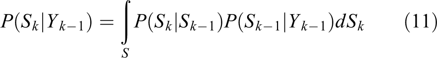
where P(S_k |Y_{k −1}) is the predictive density. The update step is given by equation (12) as

$P(S_k|Y_k)=\frac{P(Y_k|S_k)P(S_k|Y_{k-1})}{P(S_k|S_{k-1})}$

12

A particle filter approximates the posterior density by equation (13)

$P(S_k|Y_k)\approx {\displaystyle \sum _{}^{}{W}_k^i\delta (S_k-S_k^i)}$

13

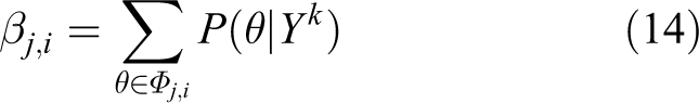
where S_k ⁱ are the particles, W_k ⁱ are the weights, k is the time step, I is the index of the particle, and Y_k is the measurement vector (observation). A problem with particle filter is that the number of particles grows exponentially with the state-space dimensionality. More efficient alternatives such as Markov Chain Monte Carlo (MCMC) ³⁹ or hybrid MCMC-particle filter may be used. Particle filters have been applied with great success to different state-estimation problems including visual tracking ^15,49 and indoor mobile robot localization. ^50,51 It represents target distribution with a set of particles (samples with states and associated importance weights), which are propagated through time to give approximation of target distribution at subsequent time steps. For mobile robots deployed in populated environment like office building, hospitals, and museums, knowledge about the position and the velocities of moving people can be utilized in various ways to greatly improve the behavior of such system. Particle filter approach allows a robot to adapt its velocity to the speed of people nearby to avoid collision. Being able to distinguish between static and moving objects can also help to improve the performance of map building and motion planning. Joint probabilistic data association filter (JPDAF) is used in assigning multiple measurements to features (objects/targets) and estimating jointly their state in the current field of view (assuming the number of objects to track is fixed). It is a probabilistic method for tracking multiple moving objects. It uses the motion model of the objects being tracked and computes a Bayesian estimate of the correspondence between detected features and the objects being tracked. In JPDAF, a joint measurement association event defined by a matrix θ is a set of measurement-event pairs (j, i) ϵ{0,1,2,…m_k } X {1, 2,…T} for m_k , measurements over T time interval for a fixed set of objects. Each θ uniquely determines which feature is assigned to which object. Let Φ_j,i denotes the set of all valid joint association events that assign feature j to object i. At time k, JPDAF computes posterior probability that the feature j is caused by object i according to equation (14):

${\beta }_{j,i}={\displaystyle \sum _{\theta \in {\Phi }_{j,i}}P(\theta |Y^k)}$

14

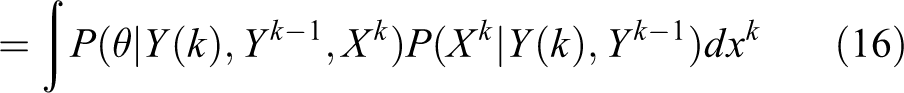
where Y(k) = (Y ₁(k), Y ₂(k),…Y_mk (k)) denotes measurement vector at time k. Y_j (k) is one of such measurement, and Y^k is the sequence of measurements up to time k. Analysis under the assumption that the estimation is Markovian, and using the laws of total probability leads to equation (15)

$P(\theta |Y^k)=P(\theta |Y(k),Y^{k-1})$

15

which simplifies to equation (16)

$={\displaystyle \int P(\theta |Y(k),Y^{k-1},X^k)P(X^k|Y(k),Y^{k-1})d{x}^k}$

16

Further simplification leads to equation (17)

$=\alpha {\displaystyle \int P(Y(k)|\theta ,X^k)P(\theta ,X^k)P(X^k|Y^{k-1})d{x}^k}$

17

α is a normalization term and m_k denotes the number of measurements at time k, and γ the false alarm rate. The number of false alarms associated with all assignment is ${\gamma }^{(m_k-|\theta |)}$ . Simplifying further finally leads to equation (18)

${\beta }_I={\displaystyle \sum \alpha {\gamma }^{(m_k-|\theta |)}}{\displaystyle \sum _{(j,i)\in \theta }P(Y_j(k)|X_i{}^k)}$

18

Neglecting measurements with low likelihood (gating) greatly reduces measurement assignment complexity. Once the posterior probability of Φ is computed (using equation (18)), it is used to assign measurements to objects. The state vector is next updated, typically using Kalman prediction or appropriate state prediction technique. ¹⁵ Within the frame work of JPDAF particle filter, Kalman filter or UKF could also be used to update the state vector, provided the dimension of the state vector is not high (less than 3D). Fox ⁵² applied adaptive particle filters to the problem of robot localization and position tracking to correct small incremental errors in robot’s odometry. The state of the robot is represented as its location and heading direction. An adaptive particle filtering with reduced sample size is employed for position tracking and global localization. Schultz et al. ⁴⁸ applied JPDAF tracking to the problem of mobile robots identifying persons walking within it vicinity using laser range scanners and particle filter for multiple tracking. Occupancy map and occlusion map are used to resolve ambiguity and detect occlusions.

MCMC-based sampling technique (Markov chains) or importance sampling makes use of priors in the application domains. The utility of Markov chains lies in the fact that by choosing a suitable transition distribution, it can be made to converge to the posterior distribution. Metropolis sampling achieves invariance ⁴⁹ resulting in transitions which are irreducible and invariant. Tracking filters are used in industrial and service robotics for motion planning, path following, and collision avoidance in addition to visual SLAM. Besides filtering approaches, there are other techniques such as fuzzy-logic ⁵³ and evolutionary and biologically inspired approaches.

Signal processing techniques

Many problems in AVs involving parameter estimation and inference can be solved as nonlinear least squares, filter-based techniques, Bayesian estimation, fuzzy-based inference, or MC-based problems. These problems arise in autonomous navigation, target tracking, localization and mapping, and multisensor data fusion. Signal processing is the basis for geolocation, distributed sensing and mapping with mobile robots, and collaborative processing. In distributed sensor networks, data management and signal detection problems must be resolved. The quality of data from different sources must also be evaluated to determine the extent of noise, disparity, and assess reliability. The classical approach to such problems may involve hypothesis testing at both the local level and the fusion center. At the fusion center, information from different remote site is combined for decision-making (inference). For example, determining thresholds for multiple decision makers (processors) in a decentralized sensor network for multiple object detection and tracking. T-test is one of the statistical hypotheses testing technique. ⁵⁴ The simplest test involves hypotheses on a population with known distribution (normal, student’s, or t-distribution) and a sample of size n. For small sample size, the student’s t-distribution is used, while for large sample size, normal distribution is used for hypotheses testing. The simplest hypothesis, the binary hypothesis, has two parts, namely, the null hypothesis and the alternate hypothesis. For a standardized parameter, the null hypothesis (H₀) states that there is no significant difference between the means of the sample and the population, and the alternate hypothesis (H₁) states that there is a significant difference between the sample mean and the population mean. The test of significance involves comparing the standardized parameter’s value with that obtained using the samples’ parameter value using either a one- or two-tail test at a given significance level. The t-test could be used to assess the quality of sensor data as a preprocessing step, or in making decision.

An F-test is any statistical test in which the test statistic has an F-distribution. ⁵⁵ The F-distribution could be used to test the hypothesis that means of normally distributed populations having the same variance are equal. The sample and population variances are known to be χ² distributed and independent, with F-ratio (vs/σ) following F-distribution. (v denotes the degree of freedom, s the standard deviation of the sample, and σ the standard deviation of the population). F-test is typically used in analysis of variance.

Hough transform is a feature extraction technique used in image processing to detect curves, lines, and other regular shape primitives in images. It represents shapes in parametric forms and a voting scheme as evidence gathering technique to detect the presence of arbitrary shapes. Except for simple regular shapes, it is generally computationally expensive since it involves setting up a look up table and searching the hough space for evidence. ⁵⁶

Turan et al. ⁵⁷ proposed an approach for estimating the parameters of a linear model using continuous kernel hough transform (a variant of hough transform based on differential equations). The approach first solves a linear equation to determine the initial parameters before applying hough transform to determine the optimum parameters. An improved version of the algorithm is proposed in Turan J and Farkas ⁵⁸ using probabilistic hough transform. ⁵⁹ Performance of the algorithm showed that it is comparable with standard least squares method in the presence of noise.

Many signals in real world are approximately sparse, meaning that while they are not sparse, can be approximated as sparse signals via compressed sensing. In compressed sensing, a signal is simultaneously measured and compressed by taking linear combinations of the signal components, resulting in fewer samples being processed. Let XЄRⁿ be the signal, and let YЄR^m the compressed signal, then the element Y_i of Y is obtained from X by equation (19)

$Y=\varphi X$

19

where [ϕ_ij ] is an m × n measurement matrix. In general, if m < n, then equation (19) is underdetermined, and in general X cannot be solved. However, using compressed sensing approach, a sparse solution can be obtained if one considers a restricted set of signals that are sparse in some representation basis. Formally, a signal X is k-sparse in a representation basis ψ Є R^nxp , if there exist an SЄR^p that is k-sparse, meaning it has at most k nonzero entries. The theory of compressed sensing provides conditions under which sparse signal can be recovered from fewer than n measurements. One such condition is the k-restricted isometry property (K-RIP), which is defined by equation (20) for k-sparse signal S, and a general matrix A

$(1-\delta )||S|{|}_2^2\le ||AS|{|}_2^2\le {(1-\delta )}_2^2||S|{|}_2^2$

20

If S is k-sparse in representation basis ψ, and the matrix A = ϕψ satisfies 2k-RIP, then X can be recovered exactly. The basic idea has also been extended to transform domain signals, sparse gradient signals, low-rank matrices, and low-dimensional manifolds. Several works ^{5,20,2,60 –62,138} provide more details on compressed sensing and its applications to mobile robotics. There are also research works on applications of compressed sensing to reduce data collection, storage, and transmission requirements in mobile robotics. These include high-resolution scene reconstruction (compressive imaging), environmental mapping ^63,64 robotic tactile skin sensing, ⁶⁵ and single-pixel camera signal processing. ² For example, tactile skins provide improvements in a robot’s awareness and manipulation abilities. ⁶⁵ Tactile sensors range from simple sensors that measure only the locations of contacts to more sophisticated ones that measure surface properties such as temperature, force, roughness, conductivity, and mechanical stiffness. For robotic perception and human-level dexterous manipulation, the main challenges are deploying large number of sensors required to meet the spatial resolution required, the resulting high data rates, noisy sensor measurements, and computational burden toward achieving real-time performance. Several strategies have been used including polling, cluster processing (local processing), and event-triggered acquisition of tactile signals. Dimensionality reduction techniques such as self-organizing map and principal component analysis are applied as a preprocessing step before classification. The next step after preprocessing is classification. An advantage of classifying in the compressive sensing domain is that dimensionality reduction is also achieved. Nguyen et al. ⁶⁴ presented an algorithm for scalar field mapping of unknown environments using groups of mobile robots and wireless sensor network for collaborative sensing over large area using compressive sensing to reduce the amount of sampling and reconstruction of missing samples. An estimate of power and communication cost is provided. Different configuration of robots executing environmental mapping tasks has also been published including those without localization support, direct communication between robots and overlay networks, and autonomous robot modeling biological systems ^66,67 and executing random walks. ^20,68,61 Collision avoidance and planning algorithms have used heuristics ⁶⁹ and evolutionary algorithms. ^{50,70 –72}

Supervised learning networks

Artificial neural networks (ANN) are biologically inspired networks mimicking the functions of the brain. ANNs offers massively and parallel distributed processing that can be used to model highly complex and nonlinear stochastic problems that cannot be solved using conventional algorithms. The basic processing element is the neuron, and the simplest ANN is the perceptron. ANNs ⁷³ are layered and characterized by the number of layers, interconnection types (fully or partially connected), topology, and learning parameters. ANNs learn on receiving some inputs (which may be labeled or unlabeled) and computationally adjusting the network parameters through simulation. At the lower layers, the network features are extracted from one layer to the next layer. At the top layer, the extracted features are generalized into a model for decision-making and inference. The generalization ability of the network depends on the nature of the problem, the input data, and the network parameters (weigh vector, learning rate, and number of neurons, etc.). There are three type of learning approaches, namely, supervised, unsupervised, and reinforcement learning (RL; learning by trial and error). Further, there are two types of models that describe the composition of the layers. The first one is the shallow learning model (networks) which is a model with few layers of compositions, for example, one or two-hidden layer models. The second type is the deep neural network (DNN) with several layers of composition, with large network parameters to be optimized. Examples of shallow ANNs are feed forward networks, radial basis functions, self-organizing feature maps, time-delay neural networks, and multilayer perceptron. ^7,74,141 There are other schemes for classification of neural networks, namely, dynamic (with memory) and static networks (without memory) for modeling nonlinearities. In dynamic networks, the output depends not only on the current inputs to the network but also on some current or previous input combination, outputs, or state of the network. Dynamic networks can be divided into feedforward and feedback or recurrent networks. The task of supervised learning is to infer a function or generalize from labeled training data set. Popular supervised learning techniques are multilayer perceptron, SVM, self-organizing feature maps (SOFM), and recurrent neural networks (RNNs). A multilayer perceptron consists of fully connected input layer where every element of the input is connected to the network, one or more hidden layers, and an output layer. The parameters of the network to be learned are the weight matrices and the bias. Data propagate from one layer to another via activation function, normally implemented as transfer function. Typical transfer functions include linear, sigmoid, and logarithm of the sigmoid function or any suitable function. The weights and bias are adjusted for each input vector via a training algorithm. The most common training algorithm is the back propagation, of which there are different variations including gradient descent, quasi-Newton’s method, and Bayesian regularization. Figure 1 shows a two-layer multilayer perception network consisting of an input, a hidden layer (layer 1), and an output layer (layer 2).

Figure 1.

A two-layer multilayer perceptron network.

Each element of the input vector P is connected to each neuron input through the weight matrix IW, or LW, input weight matrix, and layer weight matrix, respectively. The ith neuron in layer 1 has the sum of the weighted inputs and the bias as the scalar output N_i . The input layer (layer 1) implements a sigmoid transfer function (function1), and the output layer implements a linear transfer function. IW(1,1) and B(1,1) denote the input weight and bias at the input layer, respectively. LW(2,1) and B(2,1) similarly denote the layer weight and bias matrix for the hidden layer, respectively. Funct1 and funct2 denote the transfer functions for the input layer (sigmoid) and the hidden layer (linear), respectively. The output neurons are transformed according to function 2. An important architecture in robotics is RNN, which implements a dynamic ANN with arbitrary memory and generates time-varying patterns. The standard RNNs is a nonlinear dynamical system that maps sequences to sequences. In Elman (a layer RNN), there is a feedback loop with delay element around each layer except the last layer. Figure 2 shows a two-layer Elman network (D denotes a unit delay element). The delay elements stores values from the previous computations. It is thus capable of learning both temporal and spatial patterns. The Elman network has tansig (tangent of the sigmoid function) in the hidden layer and a purelin (linear) layer in the output layer. The weight vectors have dimension S by P, where S in the number of neurons in the layer, and P is the number of inputs to the layer. Layers one and two have outputs at time k defined by equations (21) and (22)

Figure 2.

A two-layer recurrent neural network.

$A1(k)=\text{tan sig}(({\text{IW}}_{1,1}*P+{\text{LW}}_{1,1})*A{1}_{(k-1)}+B_1)$

21

$A2(k)=\text{purelin}(L{W}_{2,1}*A{1}_k+B_2)$

22

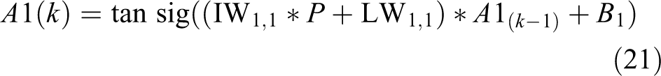
where IW_1,1 denotes the input weight matrix IW(1,1), LW_1,1 denotes the layer weight matrix in layer one LW(1,1), A1 _{k −1} denotes the (k−1)th delayed output for layer one A1(k−1), and B ₁ bias for layer 1, B(1). LW_2,1 denotes layer two’s weight for data coming from layer 1 to 2, LW(2,1), A_k denotes current output for layer one, and B₂ denotes bias for layer two, B(2) (see Figure 2). A variant of RNN, the long short-term memory ⁷⁵ is used in robotic path planning in a dynamic environment together with rapidly exploring random tree ²⁹ to reduce path fluctuations and generate realistic path to adapt the network to realistic candidate path.

Connectivity could be full, grid, hex, and mesh networks. Elman networks can approximate any function with a finite number of discontinuity with arbitrary precision. Complex networks are constructed using more hidden layers. For more description on neural networks, the reader is referred to earlier studies. ^76,74 ANNs have demonstrated robustness in control applications, and in mobile robotics, it is typically combined with analytic techniques or fuzzy systems to improve its control and navigation capabilities. Wen et al. ⁷¹ used Elman neural networks and fuzzy obstacle avoidance algorithm based on virtual force field to detect and improve robotic obstacle avoidance and navigation system. Silva et al. ⁷⁷ proposed an environmental mapping technique that combines sensors and hierarchical ANNs for recognition and classification of environmental landmarks to construct environmental maps for robotic navigation. Sharaf and Noureldin ⁷⁸ also proposed a data fusion algorithm based on radial basis function neural network that integrates GPS with inertial sensor in real time to provide positional information to land-based vehicles. It overcomes the drawbacks in using either GPS or the inertial sensor alone. It estimates positional error and improves the estimation accuracy. The resurgent of interest in ANNs in recent times is due to availability of large data set, efficient large-scale training algorithms, and powerful processors (graphics processing units (GPUs) and many core CPUs), making it possible to tackle large-scale learning problems using deep learning algorithms.

Unsupervised learning

The three main machine learning paradigms are the supervised, unsupervised, and RL. In supervised learning, each example (training sample) consists of a data sample and its class label. In unsupervised learning, only the data sample from the environment is provided and without any class label. The learning system is expected to learning the underlying data model using data samples and the class labels. In RL, the learning system learns from its environment through trial-and-error over time by interacting with the environment. There are several unsupervised learning techniques including clustering, decision trees (DTs), and Bayesian networks. Further, there are two main classes of machine learning models, namely, generative and discriminative models. A generative model captures the underlying probability distribution as well as the mechanisms used to generate data including uncertainties in data. A discriminative model in contrast generates a model (posterior probability) to differentiate between the classes or categories using supervised machine learning. It makes fewer assumptions about the underlying data model and depends largely on the quality of the data. Examples of generative models include logistic regression, conditional random fields, ^79,80 naive Bayes classifier, and Gaussian mixture models. ⁸¹

Clustering

Clustering is an unsupervised learning technique that aims at grouping data set into homogeneous units based on some criteria. It offers automated tools to discover hidden intrinsic structures in generally complex and high-dimensional configuration spaces of robotic systems. It is used in detecting structures, classification of data into subsets, and for efficient representation of data. The underlying variables (data) are typically assumed to be independent normal distributions. The three main techniques of clustering algorithms are hierarchical, partitioning, and cost function-based optimization ⁸² approaches. Hierarchical clustering includes agglomerative and divisive clustering. Partitioning clustering create k number of partitions from a given data set, each representing a set of data objects based on similarity (or dissimilarity measure). Partitioning clustering includes k-means clustering and Gaussian mixture models. In computer vision and image processing, clustering is used as preprocessing before segmentation, tracking, and object detection. Typically, a distance function is used to evaluate the quality of the resulting partitions. This could be a similarity or dissimilarity function. The objective of most clustering is to maximize intercluster distance while minimizing intracluster distance. A major challenge in clustering is dealing with outliers. Techniques like M-estimators ⁸³ could be used to achieve robustness for Gaussian-based techniques. In k-means clustering, a cluster is represented by a centroid which does not need to be a member of the cluster. Data points are partitioned into k clusters (k is user specified). The objective is to find k cluster centers and assign the data points to the nearest such that the squared distance from the cluster centroid is minimized. The algorithm starts with an initialization step where k is specified and the k centroids initialized arbitrarily. Each data point is assigned to the closest centroid. The centroids of the clusters are adjusted to the mean of the data points assigned to the centroid. This is repeated until convergence. k-means is prone to local minima and does not scale well in high-dimensional spaces. A variant of k-means, fuzzy k-means, assigns data points to clusters with certain probabilities. Each data point is given a soft assignment to a cluster with mean M_k as defined by equation (23)

$C_{tk}=\frac{\text{exp}(-\beta ||X_t-M_k|{|}^2)}{{\displaystyle {\sum }_i\text{exp}(-\beta ||X_t-M_i|{|}^2)}},{\displaystyle {\sum }_K{C}_{tk}=1}$

23

where β is the ‘stiffness parameter. In the case of k-means, C_tk has a value of one for the cluster the data are assigned, and zero for all other clusters. Both k-means and fuzzy k-means optimize the following objective functions defined in equation (24)

$J={\displaystyle {\sum }_t}{\displaystyle \sum _k{C}_{tk}}||X_t-M_k|{|}^2\text{ and the means are updated as }{M}_k=\frac{{\displaystyle {\sum }_t{C}_{tk}{X}_t}}{{\displaystyle {\sum }_t{C}_{tk}}}$

24

Closely related to clustering is expectation maximization which is a general method of finding the maximum-likelihood estimation of the parameters of the underlying distribution. It finds the model parameters that maximize the likelihood of the given incomplete data. In robotics, typical applications include pose estimation and alignment, trajectory clustering, and object tracking. ⁵⁰

Decision trees

A DT is a graphical representation of possible solutions to a decision based on certain conditions. It can be seen as a tree-based classifier. ⁶² It is similar to a tree because it starts with a single box (root), which then branches off into a number of solutions. There are several algorithms for constructing DT including those based on data attributes, univariate, multivariate, and entropy methods. ⁸⁴ In general, increasing the number of attributes and samples would improve the accuracy of the resulting classifiers. DT may be linear, nonlinear, or univariate depending on the partition function used in constructing the tree. Naumov ⁸⁵ showed that constructing an optimum DT from a decision table is NP-hard, and Rokach and Maimon ^86,139 also showed that constructing a minimal binary tree with respect to the expected number of test required to classify an unseen instance is NP-complete. It is feasible for small size problems. Consequently, heuristic methods are required for large size problems. A typical algorithm begins with all the data (root), splits the data into two subsets based on the values of one or more attributes (function of the attributes, e.g. entropy). It recursively splits each subset into smaller one until each subset contains a single class. The final subsets form the leaf nodes of the DTs. The classification process starts at the root and the data follows the directions of the decision modes until it reaches a leaf. Upon reaching a leaf, the class of the data is assigned as the class of the leaf. Sungkano et al. ⁸⁴ presented an entropy-based algorithm on humanoid goalkeeper using DT to evaluate attributes perceived by robot sensors. Each attribute uses entropy to represent its uncertainty and to calculate information gain for decision-making. DT incorporates both nominal and numeric attributes. In the case of numeric attributes, DT can be geometrically interpreted as a collection of hyperplanes, each orthogonal to one of the axis. The tree complexity is measured by one of the following metrics: total number of nodes, total number of leaves, tree depth, or number of attributes used. Each path from the root to one of its leaf can be transformed into a rule simply by conjoining the test along the paths to form antecedent part and taking the leaf’s class as the class value. For autonomous robots in dynamic environments, there is a need for replanning in case of deviations from planned path, or incremental planning given some feedback from the environment, and behavior trees derived from DT may be used. ⁸⁷ It also has the advantage of easy implementation in software and embedded systems for real-time path planning.

Bayesian networks

It is a graphical model for compactly representing probability distributions via conditional independence and captures structural relationships of data (variables). ⁸⁸ It is represented as a directed acyclic graph. The nodes are the random variables, and the edges are the direct influence between variables. It provides insight to relationship between groups of variables facilitating knowledge discovery. It defines a unique distribution in factored form as defined in equation (25)

$P\left(B,\hspace{0.17em}E,\hspace{0.17em}A,\hspace{0.17em}C,\hspace{0.17em}R\right)=P\left(B\right)P\left(E\right)P\left(A|B,E\right)P\left(R|E\right)P\left(C|A\right)$

25

A, B, C, and R are variables. It supports model selection, deals with missing variables and hidden variables. However, exact inference using Bayesian network is known to be NP-hard. ⁸⁹ Applications of Bayesian networks include SLAM ⁹⁰ and parameter estimation and inference. ^91,88 Bayesian networks have also been applied to problems in artificial perception ¹³ and pedestrian classification. ⁹² For inference, uncertainty about parameters is expressed as a probability distribution over all parameters (parameter set) using Bayes rule (equation (26))

$P(\theta |X[1],X[2],\mathrm{...}X[m\text{])}=\frac{P(X[1],X[2],\mathrm{...}X[m]|\theta )P(\theta )}{P(X[1],X[2],\mathrm{...}X[m])}$

26

X[i]s are the data samples that are assumed to be independent and identically distributed, and θ denotes the parameters of the event of interest. The left hand side of equation (26) defines the posterior distribution. The numerator of the right hand side is the product of the likelihood and the prior of the event. The denominator is the probability of the data. Graphically, it is expressed as Bayes net. ⁹¹ A dynamic Bayesian filter is used to estimate the state and pose of pedestrians based on odometry ⁹³ using IMUs. SLAM is formulated as a dynamic Bayesian problem assuming Markov process and static world assumption. The joint posterior probability is defined by equation (27)

$p(P_{0:k}\hspace{0.17em}{U}_{0:k}\dots M|Z_{1:k}^u)=\hspace{0.17em}p(M|P_{0:k})\hspace{0.17em}p({\left\{PUE\right\}}_{0:k}|Z_{1:k}^u)$

27

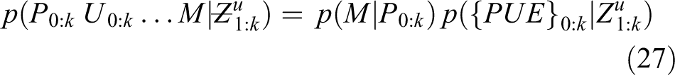
P_k denotes the pose at time k, U_k is the step transition vector at time k, $Z_k^u$ denotes the step measurements at time step k, M is the environmental map, and E_k denotes the state variable encoding the correlated errors. The notation ${\left\{P\right\}}_{0:k}$ denotes the pose estimates for between time step 0 and k. Assuming the step transition vector, U_k is determined given P_{k− 1} and P_k , the recursive formulation of (25) is given by equation (28)

$\begin{array}{l}p({\left\{PUE\right\}}_{0:k}|Z_{1:k}^u)\hspace{0.17em}\alpha \hspace{0.17em}p(Z_k^u|U_k{E}_k)\hspace{0.17em}p({PU\}}_k|{\left\{PU\right\}}_{0:k-1})\\ p(E_k|E_{k-1})\hspace{0.17em}p({\left\{PUE\right\}}_{0:k-1}|Z_{1:k-1}^u)\end{array}$

28

The recursion begins with the pose P ₀ set to an arbitrary fixed state. Post processing is applied to resolve rotation, translation, and scale transformations. The algorithm is able to construct stable 2D maps and achieve high accuracy in real time. Bayesian networks have also been applied to sensor fusion and place classification in robotics. ^94,92

Deep neural networks

A DNN employs a hierarchical structure with multiple neural networks and walks through a successive learning process layer by layer. It consists of feature detector units arranged in layers. Lower layers detect simple features and feed into the higher layers, which in turn detects more complex features. ⁹⁵ It typically consists of convolutional (CONV), restricted Boltzmann machine (RBM), or autoencoders. The availability of GPUs with very high computational throughput plays a key role in their success. DNNs have several thousands of trainable parameters. For example, Krizhevsky et al. ⁷⁶ achieved breakthrough results in 2012 Imagenet challenge using a network containing 60 million parameters with five CONV layers and a fully connected layers. It took more than two days to train the whole model using Imagenet data set on NVIDIA K40 machine. The predominant training method is backpropagation with gradient descent/ascent techniques. In recent years, DNNs have received a lot of attention following dramatic improvement in several application domains using DNN algorithms in computer vision ⁹⁶ (e.g. image classification, restoration, compressive sensing, and super resolution) and speech recognition, and natural language processing. In architectures that rely on fully connected layers, the number of parameters can grow into millions. As larger networks are considered, reducing their storage and computational cost becomes critical, especially for real-time applications, online learning, and incremental learning. DNNs have also benefitted from new development in hardware technologies such as many core processors, GPUs, ⁹⁷ and field programmable gate array (FPGA), making it possible to train these networks. There are still challenges in deploying DNN on portable devices with limited resources (memory, CPU, bandwidth, and energy). ⁹⁸ This has also brought to the fore the need for efficient training ⁹⁹ and model compression for target devices such as cellphones, FPGA, and other resource constrained systems. Several approaches have been taken toward achieving these objectives, ¹⁰⁰ including parameter pruning and sharing, low-rank factorization, and knowledge distillation. Yuan et al. ⁷² and Inoue et al. ⁷⁵ used DNNs to solve path planning problems in robotics. Despite its success, there are some criticisms of which the main one is the model’s lack interpretability compared to traditional knowledge–based approach, and its ability to predict unforeseen events which could be catastrophic.

Convolutional neural networks

The basic convolutional neural network (CNN) consists of several layers in cascade including CONV, pooling, and fully connected layers. The CONV layer is for capturing low level features like edges, corners, and lines. Each unit connects to a patch in the feature map in the previous layer through a set of kernel (filter bank). A k × k kernel with w × w input layer results in a feature map of size (w − k + 1) × (w − k + 1). The result is locally weighted and summed, it then pass through a nonlinear operation such as Rectified Linear unit (ReLU). Nonlinearity is implemented (using ReLu or Parametric ReLus) to improve model fitting. It is responsible for transforming the summed weighted input from the node into the output of the node (activation of the node). ReLu is a piecewise linear function that will output the input directly if it is positive, otherwise it will output a zero. Sigmoid and hyperbolic tangent activation functions cannot be used in networks with many layers due to the vanishing gradient problem. It is the default activation function for CNN and multilayer perceptron network. The pooling layer aims to reduce the dimension of the representation and create invariance to small shifts and distortions. It is usually placed between two CONV layers. There are two main types, namely, local and global pooling. Local pooling typically uses a local cluster (2 × 2, 4 × 4, etc.), while global pooling applies to all the neurons of the CONV layer. Typical functions are max or average pooling applied to the cluster. The top few layers are usually fully connected layers. They summarize the information conveyed by the lower layers. Usually, multiple convolution kernels are applied to the input layer resulting in multiple feature maps that collectively capture a new representation of the input. When CNNs are used for discriminative task like classification, the convolutions applied at each layer results in a decrease in the spatial extent of the feature map such that the final layer of the network represents the low-dimensional labels corresponding to the input. Figure 3 shows a diagram a three-layer CNN with nonlinearity layer. Generalization is achieved through regularization, aggressive data augmentation, and large-scale data partitioning. A major problem is over fitting and can be overcome by using more training samples. Alternatively, the dropout method is used to prevent over fitting.

Figure 3.

A three-layer CNN with successive convolutional layers. For each convolutional layer, there is a nonlinearity layer (not shown). CNN: convolutional neural network.

Different architectural configurations have also been realized to synthesize spatiotemporal features including residual block CNN and skipped connections configuration. ¹⁰⁰ Recently, a connection between CNNs and multilayer CONV sparse coding ¹⁰¹ was established. This is very important since sparsity prior is popular in signal and image processing. Ran et al. ¹⁰² proposed a “navigation via classification” framework based on a 360-degree fish-eye camera for mobile robot navigation, without the need for camera calibration, unwarping and calibration of images, and avoiding pixel-by-pixel labeling using deep CONV network. Azimuthal rotations of the cameras in 2D rotations are characterized into seven directions using rotation angles [70, 50, 30, 0, −30, −50, −70] for navigation. An end-to-end CNN based framework is proposed for the classification tasks, achieving high accuracy in a realistic setting. The network predicts potential path direction with high confidence. A major difficulty in applying CNN to robotics is acquisition of large amount of data through experimentation or simulation.

RBM and deep belief networks

RBM is a generative model (probabilistic model) with two layer bipartite undirected graphical network with a set of binary hidden units, h, a set of visible units, v (could be binary, integer, or real-valued), and connections between these two layers represented by a weight matrix W. The hidden units are conditionally independent of one another given the visible layer, and vice versa. The units of the visible layer (if binary) conditioned on the hidden layers are Bernoulli random variables. For real-valued visible units conditioned on the binary hidden units, the distribution is Gaussian with diagonal covariance. Block Gibbs sampling by sampling alternately each layer’s units in parallel given the other is applied, and the resulting expected value for each unit is its activation. RBM parameters can be optimized by performing stochastic gradient ascent on the log-likelihood of training data. Given a binary valued image (as visible unit), and assuming the binary state of each hidden unit is one, a feature detector (visible unit) is also one with probability of the hidden layer, h_i , given by equation (29)

$p(h_j=1)=\frac{1}{1+\text{exp}(-b_j-{\displaystyle {\sum }_{i\in \hspace{0.17em}vis}{v}_i{w}_{ij}})}$

29

where b_j and v_i are the bias of unit j and i, respectively. w_ij is the weight between visible unit i and hidden unit j. The reconstructed visible unit (input image) has a pixel value of one with probability given by equation (30)

$p(v_i=1)=\frac{1}{1+\text{exp}(-b_j-{\displaystyle {\sum }_{j\in \text{hid}}{h}_j{w}_{ij})}}$

30

The learned weights and biases implicitly define a probability distribution over all possible binary values of the image via the energy function. The joint configuration of visible and hidden units is defined by the energy function E(v, h) defined in equation (31)

$E(v,h\text{)}=-{\displaystyle {\sum }_{i,j}{v}_i{h}_j{w}_{ij}}-{\displaystyle \sum _i{v}_i{b}_i}-{\displaystyle \sum _j{h}_j{b}_j}$

31

Similar analysis has been carried out for Gaussian and integer value pixels. ^103,104 The hidden layers are conditionally independent of one another given the visible layer, and vice versa. The units of the visible if binary are conditioned on the hidden layers and forms Bernoulli random variables. Similarly for real-valued visible units conditioned on the hidden units, the distribution is Gaussian with diagonal covariance matrix. When RBMs are stacked together, they form deep belief network (DBN). Figure 4(a) shows a DBN where the bottom layers are directed, while Figure 4(b) shows a deep Boltzmann machine that is undirected. DBN provides unsupervised learning of hierarchically generative model. W_i and H_i denote the weight at layer i and hidden layer i, respectively. X denotes the input image. Two adjacent layers comprise a set of binary or real-valued units.

Figure 4.

(a) A deep belief network; (b) A deep Boltzmann machine.

Two adjacent layers are fully connected, but no two units in the same layer are connected. CONV DBN increases scalability by sharing the weights across all spatial locations in the image. One limitation of the two architectures is that they both ignore the 2D structure of the images. RBMs have demonstrated high accuracy in object detection and face identification. ¹⁰⁴ Deep probabilistic generative models provide probabilistically grounded framework to represent, learn, and predict under uncertainties. These include deep Boltzmann machine ^103,104,140 and DBNs. Dogan et al. ¹⁰⁵ presented an incremental and hierarchical model for task-related context modeling in robotics using RBM to model service robot’s context incrementally and achieved competitive performance compared with other techniques.

Autoencoders

Autoencoders are DNN trained to reconstruct input data at the output layer from the activations of several hidden layers. It consists of both an encoder and decoder. It is used for new representation at the encoder and to reconstruct an output at the decoder. ^106,107 Typically, all the layers are fully connected. The auto-encoding process is described mathematically as follows: An input vector XЄR^d is mapped to a latent space representation hЄD^k using a function of weight (W) and bias (b), f ₀ = ϕ(W_x + b). The code (f ₀) is used to reconstruct the input by inverse mapping with f′ = ϕ(W′f ₀ + b′) with the constrained that W′ = W^T . To prevent learning trivial identity mapping from input to output regularization is used. One regularization technique is to corrupt the input with noise as in denoising autoencoders. Figure 5 shows the general structure of an autoencoder.

Figure 5.

General structure of autoencoder.

The encoder f maps an input x to an output r through an internal representation code (h). The decoder g maps h to r. One constraint for h is to have a smaller dimension than X (achieves dimensionality reduction). ¹⁰⁸ An autoencoder whose dimension is less than the input is called an under complete autoencoder. Regularization is achieved by minimizing a loss function L of g(f(x)) for being different from x. When the decoder is linear and L is the mean squared error, an undercomplete autoencoder learns to span the same subspace as principal component analysis (PCA). Autoencoders with nonlinear encoder functions can learn more powerful functions. There are several types of autoencoders ^106,107 such as regularized autoencoders, sparse autoencoder, and variational auotencoders. Variational encoders output parameters of the distribution of the latent variables given either x or r. The encoder learns the conditional distribution. Given this conditional distribution, one can sample a random vector, z, and pass it through the decoder part of the network to output an image that looks like it is drawn from the same distribution of x. Hinton and Salakhutdinov ¹⁰⁸ applied a stack RBM to train an encoder and decoder for unsupervised nonlinear dimension reduction. After training using gradient descent algorithm, RBMs are unrolled to create a deep autoencoder which is then fine-tuned using backpropagation of error derivatives. It has also been used for image denoising, ¹⁰⁷ compressive sensing, ¹⁰⁹ and super resolution. Finn et al. ¹⁰⁶ proposed a controller for deep spatial autoencoder to acquire a set of feature points that describe the environment of the robot. First an autoencoder is applied to learn to the set of feature points associated with a particular task, and an environmental state combining object position and motion control skill associated with the state is learned via RL.

Generative adversarial network

The basic idea of generative adversarial network (GAN) is to take a collection of training examples and form a representation of their probability distribution. GANs are composed of two networks, namely, a generator and a discriminator network. The generator typically estimates the probability distribution (a generative model) and is trained to generate realistic synthetic data. ^110,111 The discriminator is a neural network trained to discriminate synthetic data from the real data. The goal of a discriminator is to be able to tell the difference between generated real images and synthetic images. It estimates the probability that the sample came from either the real or synthetic data. The two networks are trained until the discriminator is maximally confused. GANs are essentially a deterministic model as the data uncertainty is modeled by standard random variables and cannot effectively capture probabilistic distributions of the data. Tian et al. ¹¹² used a nonlinear factor analyzer as the generator network. Using alternating back propagation, the generator network learned to generate realistic images and sound. Since generator networks of GANs can contain nonlinearities and can be of any depth, the mapping can be very complex. Other GANs such as deep CONV adversarial networks have also been used for unsupervised representation learning. ¹¹³ In conditional GAN, cGAN, ^114,115 both parameters are optimized simultaneously using the loss function given in equation (32)

$L_{\text{GAN}}=E_{x->\text{pdata}(x)}(\text{log}(D(X)))+E_{y->\text{pdata}(y)}(\text{log}(1-D(G(y\text{))))}$

32

where D(x) is the data label provided by the discriminator, D, when it receives real input image as input. D(G(y)) is the label obtained when a synthesized image G(y) is input to the discriminator. The loss function drives the discriminator network to correctly classify samples as real or synthetic and pushes the generator to synthesize images that look real with the goal of fooling the discriminator. D is discarded after training, and only G is used. In cGANs, the adversarial loss is usually optimized in addition to the pixel-wise mean squared error. Among the challenges in training GANs are (a) difficulties in getting the pair of models to converge; (b) the generative model “collapsing” to generate very similar samples for different inputs; and (c) the discriminator loss converging quickly to zero, providing no reliable path for gradient updates to the generator. Mengmi et al. ¹¹⁶ presented an end-to-end training network using GAN base model for gaze prediction.

Reinforcement learning

In many problems in robotics and autonomous system, the model of the environment is not known for predictable interactions to be modeled. Instead, the robot is forced to interact with the environment over time to adapt and behave appropriately. To achieve desired autonomous system behavior in nonstationery and time-varying environment, the overall goal may be robustness and reliability rather than some form of short-term optimality. RL provides the necessary tools for developing appropriate policies. Arulkumaran et al. ¹¹⁷ and Hausknecht and Stone ¹¹⁸ provide good introduction on RL. Although RL has been applied successfully to low-dimensional environmental problems, several difficulties arise with high-dimensional problems such as high computational burden and long run times before convergence. Mnih et al. ⁴¹ made an important breakthrough by combining deep learning with RL to partially overcome the curse of dimensionality. RL defines any decision maker (learner) as an agent, and anything outside the agent as the environment. In multi-agent systems, agents must compete or cooperate to obtain the best results. And interactions between the agents and the environment are described via the states, actions, and rewards. The agent examines the state at time t, s_t , and takes a corresponding action a_t . The environment then alters the state s_t to s_{t +1} and provides a feedback reward r_{t +1} to the agent. An agent’s decision is defined by a policy, which is a mapping function (control strategy) from any perceived state, s, to actions taken, a, from that state. Given a state, a policy returns an action to perform, and an optimal policy is any policy that maximizes the expected return (cumulative discounted reward) in the environment. A value function is used to evaluate how good a certain action pair (s, a) under policies Π and Π′. There are two types of learning schemes for RL, namely, those which model the dynamics with the environment (model-based), and those which does not have knowledge of the complete dynamics of the environment (model-free), and learns the model via exploration. Examples of the former are Markov decision process (MDP) and partially observable Markov decision process (POMDP). In MDP, the next state s_{t +1}, and feedback r_{t +1} are entirely determined by the current action-state pair (s_t , a_t ) regardless of the history. Therefore, the dynamics of the RL problem is completely specified by giving all transition probabilities p(a_i , s). In POMDP, an agent receives an observation O_t ϵΩ, where the distribution of the observation p(o_{t +1}|s_{t +1}, a_t ) is dependent on the current state and the previous actions. ¹¹⁷ POMPD algorithms typically maintain a belief over the current state given the previous belief state, the action taken, and the current observation. RNNs can typically implement POMDP with arbitrary memory length. Those algorithms that do not require modeling of the dynamics include MC-based and temporal difference learning (TD). ⁷³ An episode is the length of time (T) after which the state is reset, and the sequence for states, actions, and rewards constitute a trajectory, or rollout of a policy. MC-based approaches compute updates (state-value function) after each episode. The number of episodes must be large, and every possible state must be visited several times resulting in long run times. TD makes update at the end of every step within an episode. Both MC and TD methods use tables storing value function and the corresponding state variables for every state visited and explored, making it memory intensive. This limits it to small dimensional problems in state-space. Besides using estimates of value functions and actions to improve policies (policy iteration), direct policy search methods use parameterized policies which seeks to maximizes the expected return using either gradient-based or gradient fee methods. Actor critic methods combine values functions with an explicit representation of the policy to achieve optimum behavior. The actor policy learns by using feedback from the “critic” (value function). The method provides a tradeoff of variance reduction of policy gradients with bias introduction from value function methods. Thus, actor critic methods use a learned value-function to determine optimal policy. ¹¹⁹ Zhiu et al. ¹²⁰ presented a visual navigation task for object localization and identification using visual inputs based on RL, without using any environmental map. The problem of generalization to unseen target objects in the scene based on RL, and the need to use large number of episodes for training for convergence are addressed. Successful navigation requires learning the relationship between action and the environment. A model which learns the target and the current state avoids the need to retrain the model when the scene is the same but the target has changed. A simulator was used to collect large training samples of action and reaction in different environment. Deep reinforcement learning (DRL) is based on scaling existing RL techniques to high-dimensional problems. A survey of DRL is provided in earlier studies. ^{117,118,121 –123} The powerful function approximation capabilities of neural networks and the ability to learn a low-dimensional feature representation partly account for this surge of interests. Representational and transfer learning provide another means of dealing with high-dimensional problems using CNNs. However, searching for a policy directly represented with large parameters by neural networks also suffers from local minima. The following are some of the challenges in RL: use of multiple agents in achieving desired goals and objects are challenging due to problems in communication, cooperation, and self-objective. In real-world problems, the environment may be partially observable, and noisy measurement or observations which are weakly correlated with the environments are some of the problems.

Architectures for processing in autonomous robots and mobile platforms

UAVs are popular platforms for many applications such as package delivery, search and rescue, film production, law enforcement and border control, environmental and safety monitoring (industrial accidents), and crowd surveillance. The main algorithmic problems are the high computational overheads and limited battery power. For example, about 90 min of flight time is typically available without any onboard processing. ¹²⁴ One solution to the computational over head is offloading processing to the cloud or local server via mobile edge computing. An artificial intelligence–based processing approach consisting of three-stage processing pipeline, namely, perception, cognition, and action, is typically used. Perception stage senses the environments using various sensors and interprets the sensed data in a meaningful way. Practical robots must also operate in real time. The cognition stage decides the action to take such as where to go based on the interpretation from the perception stage. The action stage performs the action command generated by the cognition stage. The action results are feedback to the perception stage for continuous operation. A review of system-on-chip architectures (SOC) for different stages of artificial intelligence–based processing pipeline is provided in Kim et al. ¹²⁵ Visual processing units (an SOC) designed for acquisition and interpretation of visual information is now available for mobile applications and optimized for small size and power efficiency. The intel Movidius Myriad2visual processing unit is an example, and interface with a complementary metal oxide semiconductor (CMOS) image sensor to capture images, preprocesses the captured images then passes the results to a pretrained neural network, and output the result while consuming less than 1 W. The forward-looking infrared (FLIR) firefly camera comes with embedded Myriad 2 vector processing unit. Their power efficiency makes them suitable for handheld mobile or drone-mounted devices. Besides the specialized processors, there are general purpose GPUs and FPGA which consume relatively large amount of power. GPUs and many core CPUs are suitable for large-scale data intensive applications, especially DNNs. The increasing availability of software frameworks for deep learning like Caffe and Teano ¹²³ ensures portability across several platforms, making deployment of neural network applications possible. For control purpose, the three processing pipeline of robotic interaction is split into two components, namely, the perception and the control loop. The control loop then combines the cognition and the action components. The functionality of a robot is encoded in the control architecture that describes how a certain task is carried out. The choice of the control architecture can have a significant impact on the way the robot deals with unstructured environment. Typical examples are finite state machines, subsumption architecture, sequential behavior computation, DTs, AND-OR-Trees, and Teleo-Reactive Programs. ¹²⁶ For indoor mobile robotics application, typical requirements are speed of approximately 2 m per second with a grid map of 10 × 10 cm square; the control commands are sent with 50 ms interval. Typical power requirements for a mobile robot is 1/10 of a Watt, with fast decision-making and small form factor.

Applications

It is predicted that by 2030, driver-assisted vehicles would be very common. Several common functionalities are expected to be provided including, autonomous navigation, target detection and tracking, communication with other entities, and self-repairing. The three main traditional approaches are control system based, vision-based, and hybrid techniques. To provide the needed processing power, they are expected to connect to cloud-based infrastructure on-the fly in a dynamic communication environment. Finally, swarm of autonomous systems are expected to cooperate and coordinate to achieve the desired outcome sometimes in real time. ^20,68 Common navigation task includes long-term (high level) planning, and low-level (local) planning. The tools require for planning are environmental maps and functionalities for detecting, tracking, obstacle avoidance, path planning tools, and high data rate communication channels. The multi-gigabit rate offered by mmWave channels for short distance communication combined with long distance communication offered by LTE (5G) channels are enablers for local and cloud computing. The functionalities from vision-based approach rely on two main technologies for image and video processing. They are 2D and 3D vision-based techniques. To improve robustness, additional sensors beside the monochrome cameras such as 3D stereoscopic cameras, GPS signals for location information, IMU, ultrasound, or LiDAR may be required. Additional constraints on the navigation tasks might have to be met. For example, UAVs are legally required to avoid landing in crowded areas. The emerging deep learning network which has demonstrated high accuracy in several application areas such as computer vision, audio processing, and pattern recognition seems a natural algorithmic choice. However, its large footprint in learning in term of computing power, and energy means offloading to a more local processing or the cloud via mobile wireless edge computing seem to offer more cost-effective approach. Another approach currently being pursued by the research community to make deep learning models scalable is model compression and development of scalable computing algorithm for mobile platforms. Mademlis et al. ¹²⁷ provided a description of the requirements and functionalities to support the use of UAVs in filming in dynamic and unstructured environment with of focus on 2D and 3D vision-based techniques. Motlagh et al. ¹²⁴ also presented UAV-based Internet of Things (IOT) platform using 2D face recognition for detecting faces in a crowd for surveillance and using mmWave for downloading and communicating with edge computing cluster for processing to achieve real-time performance. With aerial images, the main problems are the small object size, and the complex background assuming the images are orthorectified. Liu and Mattys ¹²⁸ proposed an algorithm for multiclass detection of cars in UAV images and their orientation. Bounding boxes of cars are detected using very fast sliding window detector using integral channel features and an adaboost classifier in soft cascade. The bounding box regions are further classified into different orientation and vehicle type based on histogram of oriented gradient features. Similar research work on car detection has also been reported. ^129,130 An experimental evaluation of a novel human detection and tracking algorithm is presented in the next section to illustrate the challenges in achieving real-time performance, and at the same time high detection and low false alarm rates is presented using far-infrared (FIR) videos.

Human detection and tracking using wavelet domain silhouette maps and shape outline maps

For driver-assisted vehicle especially in the night, and in highly clutter environment, early detection of pedestrians and other obstacles is very important for both pedestrians and other vehicles. Similarly, human detection and tracking is important for mobile robots in environments populated by humans. Real-time pedestrian detection poses a major challenge since traditional vision-based approaches must also cope with low-resolution images and large-scale changes. Autonomous driving and driver-assisted system for both the safety of other road users and obstacle avoidance in roads have been of interest to researcher in for more than three decades. Statistical characteristics, requirements, and algorithmic evaluations have been well discussed by Dollar et al. ¹³¹ An experimental evaluation of an algorithm for detection and tracking of pedestrians, first evaluated on CCTV footages provided by PETS 2009 challenge, is evaluated on LSI FIR database. ¹³² A brief description of the human detection part of the algorithm, based on modified version of shape outline map algorithm as originally reported in Tawiah, ¹³³ is described. The algorithm combines two feature sets, one in the wavelet domain and the other in the shape space domain. Only features in the shape domain (shape outline map similarity features) are used in the current evaluation. The processing pipeline consists of four stages, namely, preprocessing, feature extraction, candidate window localization, and classification. The algorithmic pipeline is shown in Figure 6.

Figure 6.

Block diagram of human detection algorithm.

The preprocessing stage optionally applies histogram equalization for contrast enhancement, saturation control for brightness control, and color space conversion. Feature extraction stage uses only the shape outline map to compute similarity feature vector. The shape-outline map is a global outline map of salient objects (whole object or part of an object) in the scene. It is computed after the pre-processing stage. Candidates region of interest (ROIs) within a frame are located using saliency mechanism. Candidate pedestrians within ROIs are localized via combined vertical and horizontal projected histograms of ROIs. Each ROI is also used an input to a pretrained neural network shape predictor. The predicted output is used to compute a similarity feature vector for classification. Pedestrian classification is posed as linear regression problem in the similarity feature space, and a regression network (a radial basis network) is used to train a linear classifier. LSI FIR database is a publicly available at Carlos III University of Madrid in Spain. ¹³² FIR images were collected from a vehicle driven in outdoor urban scenario. An input video frame size is 164 by 129 pixels with 14-bit precision, and all candidate ROIs are resized to 32 by 64 pixels. Table 1 shows the peak accuracy (expressed as percentages of the number of test samples) for single frame pedestrian detection after training with five-fold cross validation for different overlap ratios. The overlap between ground truth bounding box and that computed by the algorithm is expressed as a ratio. For driver-assisted pedestrian detection operating at an overlap ratio of 0.5 is acceptable. The average false positive per frame, FP, expresses the average of the false positive per frame. TN denotes the true negatives rate, and TP, the true positive rate. The high false positives (windows per frame) could be reduced using sensor fusion with radar or by tracking. Figure 7 shows some examples of detected pedestrians and sample shape outline maps. Tasks profiling was done using Matlab 2007, running on dual core CPU processor ES200 at 2.5 GHz with 4 GB RAM running Microsoft Windows vista. The shape-outline-based pedestrian detector processing pipeline achieves a processing latency of 0.41 swithout any overlap processing.

Figure 7.

(a) to (o) Detector output, global foreground outline map, and local object outline map of several framers. It is arranged from left to right in a zigzag order.

Table 1.

Confusion matrix for pedestrian detection (Peak rate).

Overlap ratio	TP (%)	FP per frame	FN (%)	TN (%)
0.5	31.00	7	69.00	20.00
0.4	60.00	7	40.00	20.00
0.3	72.00	5	28.00	20.00
0.15	91.00	6	09.00	20.00

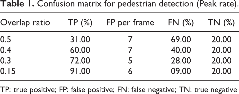
TP: true positive; FP: false positive; FN: false negative; TN: true negative

Current and future trends

Several trends can be discerned, for example, to reduce the burden on mobile platform. It is feasible to off-load computing tasks to a local processing cluster via mobile edge computing. It is also possible to use multimodal sensing to improve the accuracy of sensing tasks, for example, the use of LiDAR and FIR cameras in driver-assisted vehicles to improve detection. Similarly, distributed and cooperative or swarm-based computing is required for control and execution of complex robotic tasks over wide coverage areas. Navigation in large-scale, dynamic environments, and for long periods are still challenging, given the need for cooperation to sense and exploration of the environment for effective navigation in near real time. For example, in large-scale environmental mapping, large number of robots in groups may be deployed for rapid environmental mapping of temperature, humidity, and forest fires. For large groups of robots, current state-of-art techniques compute the paths for all robots centrally and allow for adaptation online. Further adaptive sampling robots must maintain communication links for sharing data. These impose additional constraints on the path planning algorithm. Evolutionary algorithms such as particle swarm and ant colony optimization in combination with control algorithms have been very successful. By applying compressive sensing techniques, it is possible to reduce the amount of data to be processed. Typically, the resulting problem is nonlinear and non-convex and is solved by a dedicated processing system.

The use of deep learning techniques is promising for different robotics tasks since it allows end-to-end training of models using different learning paradigms and architectures. Further, the availability of 3D teacher techniques ¹³⁴ which use 3D information from the scene to provide labeled examples to augment training data set makes it more attractive for robots to learn how to carry out tasks, interact with humans and other objects. Detection and classification functionalities are required. However, DNN has also been criticized as lacking interpretability, requiring large training and computing resources. ¹³⁵ Despite the fact that combination of deep learning and RL is very attractive for building robust autonomous systems and to large-scale problems previously not possible, it is also faced with several challenges. ¹³⁶ These include dealing with long term dependencies, temporal correlations. Mobile edge computing is a candidate solution for transmitting the large volume of data to the processing system via Bluetooth or other low power communication network, fiber-over-Wireless network to receive processed results ¹³⁷ in real time, at the same time reducing power consumption on the device platform. Several use case for this scenario has been proposed to support IOT applications. Coordination of decision in distributed processing environment where each sensor holds partial information can be modeled as a non-Bayesian version of social learning. The aim of the approach is to ensure that all agents (sensor nodes) eventually choose actions from a common prototype of randomized strategies, namely, the set of correlated equilibrium of a noncooperative game. Correlated equilibrium is a generalization of Nash equilibria ⁶³ and can be modeled as a noncooperative game-theoretic learning. ^22,70 For very specialized tasks like landmine clearing, special approaches that rely on maples navigation using chaotic trajectories avoid the use of vision techniques and coverage problems. For semiautonomous driving, there is always the need for humans in the control loop to take over in case of unanticipated scenarios, or malfunction of sensors. In future, more service robots would complement and support human activities, and be under human intelligence, or there would be a hierarchy of control with humans at the top.

Conclusions

The article has reviewed vision-based algorithms for AV navigation from the perspectives of signal processing, machine learning, statistical learning, and neural networks. Although the resulting scope is very broad compared to the traditional way of reviewing from specific subject areas (e.g. signal processing or statistical learning theory), it provides a global overview which is relevant for research. For each approach, a brief introduction is provided and, additionally review some cited references on existing literature.

Event-based visual sensors have brought in new opportunities to develop low latency and novel algorithms combining signal acquisition and processing. In AVs, combing multiple sensors data from the environment improves perception enabling more complex and coordinated task to be carried out. Challenges like continuous state estimation under uncertainties remain. Vision is a very important source of data for controlling the actions of the AVs and in executing tasks.

The general observation is that artificial intelligence–based techniques coupled with large database of examples have been successful in creating several end-to-end systems which achieves acceptable and constantly improving performance. The trend toward deep learning model compression is making headway in achieving small footprints applications suitable for low power and latency systems.

Challenges such as distributed processing of signals and decision-making with minimum communication infrastructure, low power, migrating applications to IOT devices, privacy, and security of devices must be contended with. Additional challenges occur in AVs navigating in highly dynamic environments, as well as management of large cooperative mobile robots, and their interactions.