Sage Journals: Discover world-class research

Abstract

The study is concerned with the problem of online planning low-cost cooperative paths; those are energy-efficient, easy-to-execute, and low collision probability for unmanned surface vehicles (USVs) based on the artificial vector field and environmental heuristics. First, we propose an artificial vector field method by following the global optimally path and the current to maximize the known environmental information. Then, to improve the optimal rapidly exploring random tree (RRT*) based planner by the environment heuristics, a Gaussian sampling scheme is adopted to seek for the likely samples that locate near obstacles. Meanwhile, a multisampling strategy is proposed to choose low-cost path tree extensions locally. The vector field guidance, the Gaussian sampling scheme, and the multisampling strategy are used to improve the efficiency of RRT* to obtain a low-cost path for the virtual leader of USVs. To promote the accuracy of collision detection during the execution process of RRT*, an ellipse function-based bounding box for USVs is proposed with the consideration of the current. Finally, an information consensus scheme is employed to quickly calculate cooperative paths for a fleet of USVs guided by the virtual leader. Simulation results show that our online cooperative path planning method is performed well in the practical marine environment.

Keywords

Online cooperative paths planning unmanned surface vehicles artificial vector field Gaussian sampling elliptic bounding box

Introduction

The online path planning (OPP) module is essential for unmanned surface vehicles (USVs) when unreliable or delayed communication links between human and USVs exist. The OPP problem for USVs faces challenges, for example, limited computational ability of the shipborne computer, limited communication bandwidth and the strong external interferences, unstructured or changeable environmental information, and complicated motion constraints of USVs.

Besides, USV missions are typically performed under the strict energy constraint and the current interference. However, the changes in the velocity and direction of the current are generally small in a certain spatial–temporal range, and the characteristics can be used to improve the energy efficiency of USVs by executing downstream paths when USV moves at a relatively small speed compared to the speed of the current. Sometimes, USV enhances the motion stability by executing countercurrent paths. But, USV has a weak ability of the lateral current resistance. Therefore, one of the planning objectives is to generate paths containing many downstream sections and a small amount of countercurrent sections with few transverse parts. Besides, the path length, path smooth, and obstacle-avoidance (OA) requirements are also important.

High efficiency is the first requirement of an OPP scheme to quickly response to the changes of USV states and environmental information. Since USVs are underactuated, and some control variables are complex. Meanwhile, the sophisticated motion model and parameters are rare. Thus, computing a desirable and feasible trajectory can be very difficult by directly adopting control-based methods.

Meanwhile, the cooperative path planning problem is more complicated than that of planning for a single path. If we plan paths for each USV separately, the computational complexity is huge, and even deadlock problem exists.

The motivation of the research is to online plan cooperative paths, which are energy-efficient, smooth, and low collision probability.

Up until now, a number of notable results on USV OPP problem have been reported in the literature. The forward-looking path planning methods are applied more often than the behavior-based method, which is short-sighted.

The artificial potential field (APF) method computes a vector field by calculating an attractive force field from the goal and a repulsive force field from obstacles. Then, USVs can navigate using gradient descent to follow the potentials in real time. However, APF has difficulties when USV sails in narrow passages, and it does not consider the motion model.

The rapidly exploring random tree (RRT) algorithm accelerates the planning process by avoiding the explicit and accurate modeling of the environment.¹ Moreover, RRT works efficiently for systems with differential constraints and nonlinear dynamics, because RRT does not require exact connection between states. Particularly, RRT handles constraints piecewise and deals with motion errors or sudden situations according to real-time feedback by expanding the path tree incrementally. Since the path refinement is crucial, the optimal RRT (RRT*) is chosen as the basic path planning method. RRT* ensures that nodes are reached through a minimum cost path by “rewiring” the path tree.

The basic contradiction in path refinement is the one between the limited online time and path optimality. Because the probabilities of sampling spaces containing the optimal solution are not assessed, RRT* converges slowly to the optimal path, and the OPP module is performed in a low bandwidth along with the autonomy hierarchy. Thus, the efficiency of RRT* is required to be improved. The optimal result is hard to be achieved online. Thus, the heuristic schemes were extensively researched to promote the planning speed of the RRT method.² A Gaussian sampling method was applied to obtain more environmental information using less samples for exploration than random sampling scheme to improve the OA ability of RRT.³

The environmental current field can be used as the heuristics for designing an energy-efficient path planning method. A numerical ocean model was constructed by Holland and McWilliams.⁴ A method was introduced by constructing the model for the current with the B-spline surface.⁵ The current disturbance was considered by Singh et al.⁶ to plan energy-efficient paths. The current was considered during the path searching process to plan for paths with minimum energy expenditure.⁷

An approach was proposed to guarantee the existence of a path in strong current fields by combining a cost function and optimization methods.⁸ An energy-efficient path planning algorithm was proposed to address the challenges with the presence of the current.⁹ A path planning method was proposed for USV under uncertain, inaccurate, and dynamic marine information.¹⁰ An energy-efficient path planning algorithm was proposed to consider the current based on the A* method, and a realistic case of an autonomous underwater glider surveying the Western Mediterranean Sea was considered.¹¹ The problem of optimizing the energy cost was considered by Alvarez et al.¹² The USV speed was computed according to the input USV velocity and the current velocity by Garau et al.¹³

The environment was modeled by the artificial vector field according to the known information by Lawrence et al.¹⁴ and Chen et al.¹⁵ A vector field was constructed by following a Dubins path based on the Lyapunov stability principle.¹⁴ The path was defined as the intersection of two surface functions.¹⁶ A continuous time-variant vector field was proposed based on the n-dimensional curve, which was defined by the intersection of n − 1 curved surfaces.¹⁷ A Lyapunov vector field was produced to control robots to stably convergence to a cycle behavior.¹⁸

The common USV formation control strategies include behavior-based approach, leader-follower approach, virtual structure approach,¹⁹ and the methods based on consensus theory and graph theory.²⁰ The consensus theory was proposed to unify the leader–follower, behavior-based, and virtual structure approaches into the framework of consistency theory.²⁰ The cooperative formation control based on consistency algorithm can realize multichannel compound control to avoid obstacles.

The formation control problem for USVs was addressed by a distributed strategy based on virtual structure strategy.²¹ A hierarchical control framework and relevant algorithms were proposed for autonomous navigation of USVs.²² A three-layered architecture was devised for the real-time implementation of USV OA problem.²³ An improved APF method was responsible for avoiding obstacles smoothly.²⁴ An improved APF method was employed using ring-shaped repulsion for collision avoidance and OA.²⁵ The full-state regulation control problem for USVs under disturbances was solved by Wang et al.²⁶ Accurate trajectory tracking control problem of USVs disturbed by complex marine environments was addressed by Wang et al.^27,28

The novel contribution of the study is summarized below: (1) to effectively guide the USV path planning process, an artificial vector field is applied by following the reference path and the current. The vector field is used as the heuristics to plan for energy-efficient and low-cost paths. (2) The vector field following Gaussian sampling and multisampling schemes is used to improve the efficiency of RRT* to obtain a low-cost path for the virtual leader of USVs. The cooperative path planning strategy is investigated based on the distributed consensus. (3) A bounding box construction method is presented to improve the collision detection (CD) accuracy by taking the velocities of USVs and the current into account.

Online path planning framework for unmanned surface vehicles

Online path planning framework

The framework of the cooperative paths planning system is built based on the virtual structure method and the information consensus scheme. We first plan paths for the virtual leader, then a follower computes its path according to the positions and velocities of the virtual leader and other followers based on the information consensus.

Figure 1(a) shows the core hardware and software modules of the OPP system for the virtual leader. To maximize the given information, a global reference path is planned according to the known obstacle and current information. The central controlling module is mainly in charge of the global reference path planning, submodules scheduling, and the synchronization management. The numbers at the right bottom of modules show the sequential logic of the system. The scheduling sequence of the OPP module is the second. The OPP module plans low-cost paths locally using real-time USV states and environmental information.

Figure 1.

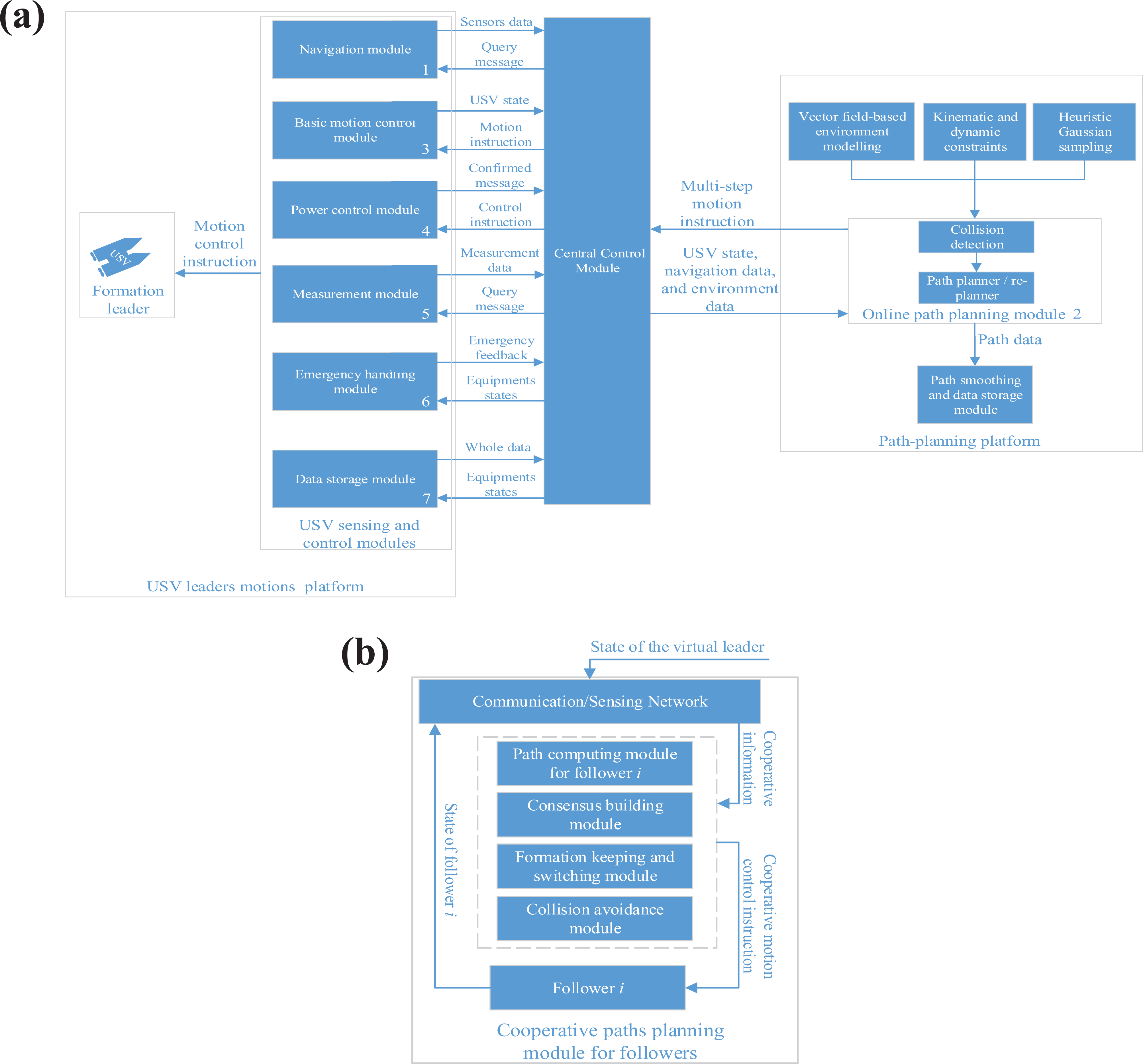
Framework of the USVs cooperative paths planning system. (a) Framework of path planning for the virtual leader and (b) framework of path planning for followers. USV: unmanned surface vehicle.

To adapt the reference path, we model the environment by constructing a vector field that follows the global path and the current. To satisfy the feasibility of the path, we planned paths’ online subjects to the USV motion model. To plan energy-efficient paths, the directions of USV motion and the current are considered.

The OPP method is proposed based on the model predictive control scheme. The most recent data are not necessarily the most suitable in a real-time system.²⁹ Thus, the OPP module sends a committed path to the central controlling module at specified update points, and the committed path is an unchanged one that is not influenced by the OPP process. The time difference between two adjacent update points (δ_e ) is the duration of the execution domain. The OPP module predicts a local path in the prediction time domain δ_c . The virtual leader is supposed to move along the committed path, and the adapting section subsequent to the next updated point is refined in δ_e time. If the reference path intersects with the perception boundary, then the intersection point closest to the goal is chosen as the subgoal of the local planning iteration, else, the nearest waypoint of the reference path is selected as the subgoal. Followers compute paths after cooperative information from the virtual leader and other followers are obtained. Figure 1(b) shows the cooperative paths computing framework for the followers.

Unmanned surface vehicle motion model and constraints

Figure 2 shows the Earth-fixed inertial frame {i} and the body-fixed frame {b}. The positive direction of the X-axis of frame {b} coincides with the USV heading direction, and the origin locates at the barycenter of USV.

Figure 2.

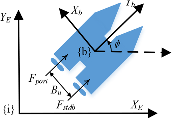
Schematic of USV kinematic and dynamic models. USV: unmanned surface vehicle.

The experimental motion model is as follows

{\begin{cases} x' = u \cdot cos ψ - v \cdot sin ψ \\ y' = u \cdot sin ψ + v \cdot cos ψ \\ ψ' = r \\ u' = \frac{m_{22}}{m_{11}} \cdot v \cdot r - \frac{d_{u}}{m_{11}} \cdot u - \sum_{i = 2}^{3} \frac{d_{{u i}}}{m_{11}} \cdot | u |^{i - 1} \cdot u + \frac{1}{m_{11}} \cdot τ_{u} + \frac{1}{m_{11}} \cdot τ_{w r} (t) \\ v' = \frac{m_{11}}{m_{22}} \cdot u \cdot r - \frac{d_{v}}{m_{22}} \cdot v - \sum_{i = 2}^{3} \frac{d_{{v i}}}{m_{22}} \cdot | v |^{i - 1} \cdot v + \frac{1}{m_{22}} \cdot τ_{w r} (t) \\ r' = \frac{(m_{11} - m_{22})}{m_{33}} \cdot u \cdot v - \frac{d_{r}}{m_{33}} \cdot r - \sum_{i = 2}^{3} \frac{d_{{r i}}}{m_{33}} \cdot | r |^{i - 1} \cdot r + \frac{1}{m_{33}} \cdot τ_{r} + \frac{1}{m_{33}} \cdot τ_{w r} (t) \end{cases}

where x, y are the position vectors; ψ is the yaw angle; [u, v, r]^T are the corresponding velocity vectors; d_u , d_v , d_r , d_ui , d_vi , and d_ri (i = 2, 3) denote the hydrodynamic damping in surge, sway, and yaw. m_ii (i = 1, 2, 3) denotes the mass parameters, including added mass contributions, and they are derived according to Mousazadeh and Kiapey,³⁰ τ_u = (F_port + F_stdb ) denotes the surge force, τ_r = (F _port − F _stdb)·B_u /2 is the yaw moment, F _port and F _stdb are the thrusts from the propellers on the port side and starboard side, respectively, B_u is distance between the propellers

{\begin{cases} m_{11} \approx m + 0.05 \cdot m \\ m_{22} \approx m + 0.5 \cdot (ρ \cdot π \cdot D^{2} \cdot L) \\ m_{33} \approx 0.083 \cdot m \cdot (L^{2} + W^{2}) + 0. 042 \cdot (0.1 \cdot m \cdot B^{2} + ρ \cdot π \cdot D^{2} \cdot L^{3}) \end{cases}

where the coefficients are derived by Mousazadeh and Kiapey.³⁰ The length L of the hull is 1 m and the width W is 0.25 m, the average depth of underwater penetration D is 0.3 m, and ρ is the water density. We set: d_u2 = 0.2d_u , d_v2 = 0.2d_v , d_r2 = 0.2d_r , d_u3 = 0.1d_u , d_v3 = 0.1d_v , and d_r3 = 0.1d_r . The τ_wr (t) is the torque of current on hull.

Online path planning scheme

Global path optimizing

To maximize the given environmental information, a global reference path is optimized using the A* method according to the known environmental information. The A* method is resolution-complete, where the path corresponds to a sequence of consecutive blank cells between the starting cell and the goal cell. The side lengths of the cells are defined as η_A = v _min * Δt, where v _min is the minimum velocity of USV and Δt is the extension step duration of RRT*. The heuristic cost function for A* is defined as follows

H (g_{i}) = dis (g_{i}, goal) + angle (g_{i}, c_{i})

where g_i denotes the center of a cell, dis(g_i , goal) is the distance from g_i to the goal, and angle(g_i , c_i ) is the angle between the directions of exploration and the current. The exploration direction is the direction of the segment from a waypoint to a g_i .

The A* method assumes that USV is omnidirectional without considering the motion characteristics of USV. Thus, the reference path is just used as a guidance of OPP process, and it should not be complicated and zigzagged. We try to prune redundant waypoints sequentially. The pruning start point is selected as the first waypoint and the end point is defined as the third point initially. If the line between the start and end points is collision-free, then the intermediate point is deleted and the end node moves to the next point. The iteration is performed until the line between the start and end points intersects with obstacles. Then, the next start point is chosen as the last end point.

Polygonal paths cannot represent the characteristics of USV motion. Thus, we smooth the reference path via Dubins curve, which is proven to be the shortest distance between vectors under the minimum turning radius constraint via using geometric analysis. We assume that the USV moves from a configuration to another one according to the Dubins maneuver. Dubins curve is composed of arcs with the minimum turning radii and their common tangents. The waypoints in the vector model are known as tangent points acquired by differential geometry.

Artificial vector field-based environment model

A vector field following the Dubins path and the current is constructed in the discrete environmental map to guide the OPP process. The magnitude of the vector at each position is related to the expected velocity of USV at the grid. The bigger the distance from USV to the reference path, the bigger the speed of USV. The expected magnitude of USV velocity is calculated as follows

v_{E} = min {λ d_{u r}, v_{max}}

where d_ur is the distance between USV and the nearest waypoint of the reference path, the weight λ is set as 0.5, v _max is the maximum speed of USV, and it is set to be10 kn (5 m/s).

According to Lawrence et al.,¹⁴ we define a positive definite and continuous derivable potential energy function V_F (r) that satisfies the following conditions: if USV is not on a path Φ, then V_F (r) > 0; if USV is on Φ, then V_F (r) = 0; and only if V_F (r) = 0, then ∂V_F (r)/∂r = 0.

If the motion characteristics of USV obeys r′ = f(r, t, λ), where f(r, t, λ) is the vector field following the path Φ and f(r, t, λ) = −[(∂V_F (r)/∂r) Γ(r, t, λ)]^T + Θ(r, t, λ) + γ(r, t, λ). The vector field guarantees USV to converge to the path Φ, where Γ(r, t, λ) is a n × n semipositive definite symmetric matrix, and only if USV is on the path, Γ(r, t, λ) = 0, otherwise, Γ(r, t, λ) > 0; (∂V_F (r)/∂r) Θ(r, t, λ = 0; (∂V_F (r)/∂r) γ(r, t, λ)) = −∂V_F (r)/∂t.¹⁴

The conclusion can be proved as follows: V_F (r, t, λ) = (∂V_F (r)/∂r) r + ∂V_F (r)/∂t = (∂V_F (r)/∂r) f(r, t, λ) + ∂V_F (r)/∂t, thus ${V^{'}}_{F}$ (r, t, λ) = −(∂V_F (r)/∂r) Γ(r, t, λ) (∂V_F (r)/∂r) ≤ 0, only if USV is on the path Φ, then Γ(r, t, λ) = 0. Thus, the vector field is negative semidefinite. According to the Lyapunov theorem, USV can converge to Φ. In the vector field, −[(∂V_F (r)/∂r) Γ(r, t, λ)]^T provides the force on the direction of negative gradient of vector field to help USV converge to the curve Φ. Θ(r, t, λ) provides the force perpendicular to the gradient direction of the vector field and its sign determines the direction of USV that moves along the curve Φ. γ(r, t, λ) is the compensation for the time-varying change of vector field or the compensation for the USV speed on the curve, and it deflects the vector field to the direction of the USV velocity.

It is difficult to define a vector field that can follow an arbitrary style of curve. Thus, we smooth the reference path via Dubins curve. Then, we design a vector field that follows the Dubins path. We define two kinds of vector fields that follow arcs and segments, respectively, then we integrate the two vector fields to follow an arbitrary Dubins path.

When the vector field follows arcs, the potential field function is defined as $V_{F} = 0.5 {(r (t) - R (t))}^{2}$ , where $r (t) = \sqrt{{(x - x_{0})}^{2} + {(y - y_{0})}^{2}}$ , and (x, y) is the USV position, (x ₀, y ₀) is the center of the horizontal maneuver arc. $\frac{\partial V_{F}}{\partial r} = (r (t) - R (t)) {\hat{r}}_{\nabla}$ . We set $Γ (r, t, λ) = \frac{I_{2 \times 2}}{χ (r, t, λ)}$ , $Θ (r, t, λ) = \frac{λ_{1} {\hat{r}}_{Δ}}{χ (r, t, λ)}$ , and $γ (r, t, λ) = \frac{λ_{2} {\hat{r}}_{\nabla}}{χ (r, t, λ)}$ , where $χ (r, t, λ) = \frac{\sqrt{{(r (t) - R (t) - λ_{2})}^{2} - λ_{1}^{2}}}{v_{E}}$ .

The ${\hat{r}}_{Δ}$ guides USV to move on the direction of the tangent of the curve, whereas ${\hat{r}}_{\nabla}$ is on the gradient descent direction and it guides USV to move toward the curve, and ${\hat{r}}_{Δ} = \pm \frac{1}{r} (y_{0} - y, x - x_{0})$ , ${\hat{r}}_{\nabla} = \frac{sgn (R - r (t))}{r (t)} (x - x_{0}, y - y_{0})$ , where the function sgn(R – r(t)) means the sign of the item R – r(t). The parameter λ ₁ is the weight of the influence of the yaw motion on the velocity direction, and λ ₂ is the weight that influences the change of the vector field with time.

Therefore, we can get $f (r, t, λ) = \frac{- (r (t) - R (t) - λ_{2}) {\hat{r}}_{\nabla} + λ_{1} {\hat{r}}_{Δ}}{χ (r, t, λ)}$ , where $| f (r, t, λ) | = v_{E}$ . The vector direction is as $φ_{d} (t) = arctan \frac{sgn (R (t) - r (t)) (- (r (t) - R (t)) + λ_{2}) (y (t) - y_{o}) \pm λ_{1} (x (t) - x_{o})}{sgn (R (t) - r (t)) (- (r (t) - R (t)) + λ_{2}) (x (t) - x_{o}) \pm λ_{1} (y_{o} - y (t))}$ .

Figure 3(a) shows the vector field following an arc, and the parameters of λ ₁ and λ ₂ are values to make the vectors to return to the path and steer to the direction of the path. Figure 3(b) shows that the trend of vectors is more likely to follow the velocity of USV (steering to the direction of the path) on the path than to return to the path along with the increment of λ ₁. The vectors close to the path are nearly parallel to the path without pointing at the path. That makes USV moves parallel to the path before it returns to the path. The velocity following the trend of vectors decreases after λ ₁ is reduced, as shown in Figure 3(c), the vectors are more intended to point at the path than following the velocity parallel to the tangent of the path. Figure 3(d) shows that after λ ₂ is increased, the vector field is more intended to return to the path than turning to the direction of the path. We set λ ₁ to be 15 and λ ₂ to be 0.3.

Figure 3.

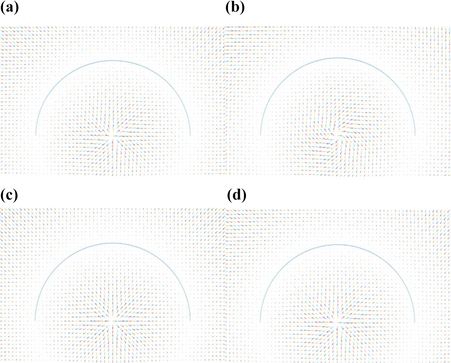
The influence of the parameters λ ₁ and λ ₂ of the vector field. (a) The parameters λ ₁ = 5 and λ ₂ = 0.3, (b) the parameters λ ₁ = 15 and λ ₂ = 0.3, (c) the parameters λ ₁ = 0.1 and λ ₂ = 0.3, and (d) the parameters λ ₁ = 5 and λ ₂ = 5.

When the vector field follows a segment path, the potential energy function in defined as V_F = 0.5r(t)², where r(t) is the distance between USV and the segment path. $\frac{\partial V_{F}}{\partial r} = r (t) {\hat{r}}_{\nabla}$ , $r = \sqrt{{(x - x_{0})}^{2} + {(y - y_{0})}^{2}}$ , ${\hat{r}}_{\nabla} = \frac{1}{r} (x - x_{0}, y - y_{0})$ , and ${\hat{r}}_{Δ} = \pm \frac{1}{r} (y_{0} - y, x - x_{0})$ , where (x ₀, y ₀) is the projection of USV on the segment path. In the vector field function, we define $Γ (r, t, λ) = \frac{I_{2 \times 2}}{χ (r, t, λ)}$ , $Θ (r, t, λ) = \frac{λ_{3} {\hat{r}}_{Δ}}{χ (r, t, λ)}$ , $γ (t) = 0$ , thus, $f (r, t, λ) = \frac{- r (t) {\hat{r}}_{\nabla} + λ_{3} {\hat{r}}_{Δ}}{χ (r, t, λ)}$ , where $χ (r, t, λ) = \frac{\sqrt{r {(t)}^{2} + λ_{3}^{2}}}{v_{E}}$ and $| f (r, t, λ) | = v_{E}$ . The directions of vectors in the field can be calculated as $φ_{d} (t) = arctan \frac{- r (t) (y (t) - y_{o}) \pm λ_{3} (x (t) - x_{o})}{- r (t) (x (t) - x_{o}) \pm λ_{3} (y_{o} - y (t))}$ . The weight λ ₃ is set by the expected motion of USV following the reference path, and it is set to be 0.1.

Figure 4 shows the vector fields with different parameters. Figure 4(a) shows that the vectors can point to the path while turning to the direction of the path. Figure 4(b) shows that the vector field has a bigger intention of returning to the path than steering to the direction of the path when λ ₄ is reduced, λ ₄ is set to be 2 in the study.

Figure 4.

The influence of the parameter λ ₄ on the vector field. (a) The parameter λ ₄ = 2 and (b) the parameter λ ₄ = 0.2.

The vectors at the intersections of a segment and a circle on the Dubins path are the resultant vectors of the one following the segment and the one following the circle. The combined vectors exist within a scope around the intersection. Figure 5 shows the vector field following the combined path of segment and circle. Figure 5(a) shows that the vectors at the intersection area are influenced by the segment and arc, and Figure 5(b) shows the resultant vectors.

Figure 5.

The vector field following the Dubins path. (a) Vectors at the intersection area of segment and arc and (b) the resulting vector field.

To consider the current in the definition of the vector field, the vector field is integrated with the current field. The vector field is proven to guide the USV to follow paths stably. However, the vector field does not consider the USV motion model and the OA problem. Thus, the vector field is used as the heuristics of OPP.

In a USV system, the CD problem between formation members especially when changing formation is necessary to be solved. A formation potential field is designed based on the spring-damping model that consists of a “piston” and a “Hooke spring” with a nonzero static length. When the piston is pressed inward from the balance point, the spring will produce a repulsive force to prevent the piston from moving forward. When the piston moves forward to a certain distance, the spring resistance will prevent USV from moving forward. On the contrary, the spring will produce a pulling force to pull the piston back to the balance point. The principle is applied among the members to keep the activities of each USV within their own allowable range and ensure the formation of the team and the safety of the members. According to Hooke’s law, the elastic potential field between USVs is as follows

{\begin{cases} U_{i j}^{h} = \frac{1}{2} k_{i j}^{h} r_{i j}^{2} \\ F_{i j}^{h} = k_{i j} r_{i j} \end{cases}

where $U_{i j}^{h}$ is the elastic potential field between USV _i and USV _j , $k_{i j}^{h}$ is the elastic potential field coefficient (it is set to be 25). r_ij = D_ij – E_ij , where D_ij is the actual distance between USV _i and USV _j while E_ij is the expected distance between USVs.

The elastic forces between members are computed as $F_{i}^{h} = \sum_{j = 1, j \neq i}^{n} k_{i j} F_{i j}^{h}$ , and if the distance between USVs is lower than a threshold (0.5), the force is set to be infinity. The related acceleration to the force is set as $F_{i}^{h} / m$ , where m denotes the weight of USV. Meanwhile, the OA priorities of USVs are determined before the sail begins. The low-priority members give way to the high-priority USVs to avoid collisions.

Heuristic path tree extension scheme

Heuristic cost function

An RRT*-based OPP method is proposed to plan paths for the virtual leader. The vector field is used as heuristics in the sampling process of RRT*. A heuristic path tree extension scheme is presented to improve the path quality and improve the path planning efficiency of RRT* in obstacle complex areas.

RRT* converges slowly to the optimal path. Thus, a heuristic RRT* method is proposed to efficiently search for and refine paths. The direction of path exploration is controlled and adjusted during the path exploration process of RRT*. To refine paths, a cost distance is defined by considering the energy expenditure, execution difficulty, and safety, as follows

C dist (q_{i}, q_{j}) = (1+ γ_{l} \cdot (1 + cos α_{T}) + \frac{1}{max_{Obs \in S} {0, γ_{o} \cdot (d_{obs} - v_{i} \cdot Δ t \cdot cos α_{i})} + ε} + γ_{y} \cdot | sin α_{y} |)) \cdot dist (q_{i}, q_{j})

where α_T is the angle between the extending direction (from q_i to q_j ) and the USV velocity vector, and α_T is considered to guide the algorithm reducing the numbers and angles of turns on paths. The variable d _obs is the minimum distance from the linear path between q_i and q_j to obstacles within a scope S centering at USV, and α_i is the angle between extending direction and the direction from q_i to the center of the nearest obstacle and v_i is the resultant velocity of the velocity of USV on the path between q_i and q_j and the velocity of the current, and the item v_i ·Δt·cosα_i is the estimated distance that USV moves toward an obstacle and max{0, γ_o (d _obs − v_i ·Δt·cosα)} is equal to 0 if the braking distance is not enough, ε is a small number (set to be 0.01) that avoids the numerator of the second item being 0. Thus, the cost distance is rather big, if the linear path between two nodes gets very close to an obstacle. α_y is the angle between the extending direction and the direction of vectors in the vector field. The dist(q_i , q_j ) is the Euclidean distance between q_i and q_j . The angles are limited as 0 ≤ α_T ≤ π, 0 ≤ α_i ≤ π, and 0 ≤ α_y ≤ π. We set γ_l = γ_y = 0.3, γ _o = 2.5.

Thus, the cost distance definition considers the planning objective as follows: the first item considers the tortuosity of the path; the second item considers the collision probability of the path; the third item considers the energy efficiency of the path through the vector field that takes the current into account; and the formula also considers the path length by the variable dist(q_i , q_j ).

Heuristic sampling scheme

RRT* also has difficulty in searching for paths in obstacle-complex areas. Thus, a heuristic sampling scheme is proposed based on a Gaussian function³ and the transition-based RRT method² to help RRT* generating reasonable samples to improve its path searching and refining ability.

The Gaussian sampling scheme is used to generate samples near the obstacle boundary to find a short OA path quickly according to the sampling of historical information. It spawns several samples and chooses the one that lies close to obstacles. The method may accelerate the OA path planning procedure because the samples near obstacles may help to find OA paths; the computational complexity of spawning an obstacle-free sample is much lower than that of the path extension process. The Gaussian function is defined as follows

φ (c, σ) = \frac{1}{{(2 π σ^{2})}^{\frac{d}{2}}} \cdot e x p (- \frac{c^{2}}{2 σ^{2}})

where σ is the standard deviation of the Gaussian distribution, it is determined by the smallest distance tolerance of USV toward obstacles, we set it like two times of the USV length.

We define a function for assessing the probability of a sample q_s on the boundary of an obstacle as $f (q_{s}, σ) = \int_{y \in D_{b}} obs (y) \cdot φ (q_{s} - y, σ) d y$ , where obs(y) = 1 if a configuration y locates at an obstacle-occupied area, and obs(y) = 0 if y is in an obstacle-free area, and the integral scope is performed within an obstacle boundary-blurring domain D_b . The radius of D_b is set as three times of σ. The function of f(q_s , σ) is used for blurring the obstacle boundaries as the application of Gaussian smoothing in the image processing area. The weights of the obs(y) are given by the Gaussian function φ(q_s − y, σ). The closer a configuration y to the configuration q_s , the higher the weight. The weights reflect the similarity of q_s to the configuration y.

The Gaussian function-based fuzzy value of q_s is defined as g(q_s , σ) = max{0, f(q_s , σ) − obs(q_s )}, if q_s is within the obstacle-occupied area, then g(q_s , σ) = 0, else g(q_s , σ) = f(q_s , σ). The function value of g(q_s , σ) is used as the fuzzy value of a sampled configuration q_s to assess the probability of q_s locating near the boundary of an obstacle in an obstacle-free area.

The path tree extension steps 1 and 2 are executed iteratively, as follows:

A sample q_s is spawned randomly and the nearest path tree node q_n is searched according to formula (6).

The nearest node q_n is tried to extend according to the vector at q_n when a randomly generated number rand ∈ [0, 1] is lower than the threshold p (0.5). If the extension succeeds, then a new node is added to the path tree and the locally topologic path tree refinement (rewiring) is executed as the RRT* method.

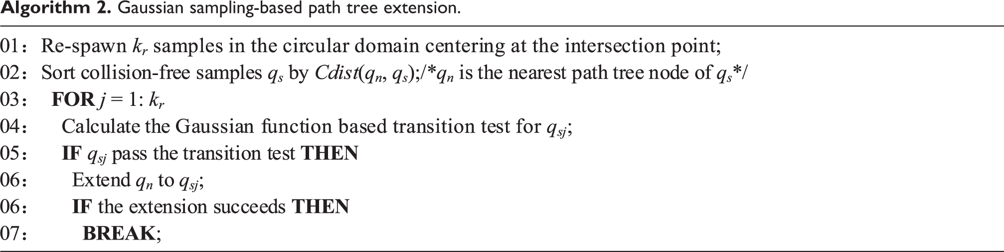
If an extension collides with an obstacle, then the algorithm keeps the intersection point (C_p ) of the extending section and the obstacle, and the OA path planning process is started as: several samples q_s are respawned in the circular resampling domain centering at C_p .

The collision-free samples are sorted by the cost distances from the nearest path tree node q_n of a sample (q_s ) to q_s in the ascending order, and the Gaussian function-based fuzzy values of samples are tested by the transition function that is defined as follows

p (q_{s}) = exp (- \frac{1 - g (q_{s}, σ)}{K})

where K is a constant value (set to be 3) used to control the changing range of p(q_s ). A random number R_T ∈ [0, 1] is chosen. If R_T is lower than p(q_s ), then the q_s is kept and q_n is tried to extend to q_s , else go to the next sample. The iteration is executed until an extension succeeds. If all the samples are tried, then return to step 1.

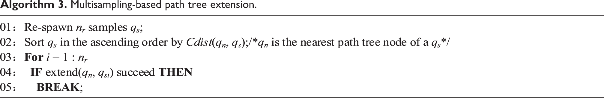
Else, a multisampling-based heuristic extension process is executed if rand exceeds p as follows.

Several samples q_s are respawned in a resampling domain around q_n . The collision-free samples are sorted by the cost distances from the nearest path tree node q_n of a sample (q_s ) to q_s in the ascending order. Next, q_n tries to extend to q_s in order until an extension succeeds or all the extensions fail. Then, the algorithm returns to step 1.

The extension procedure of path tree has some randomness, which aims to search for high-quality paths by consideration of various candidate paths in a wider range. Figure 6 shows the illusion of the Gaussian sampling process, where q _new is the newly generated path tree node and d is the radius of the resampling domain. The extension step length η = v_U Δt. The motion constraints are taken into account during the path extension procedure. Thus, the feasible extendable domain for a path tree node is fan shaped. We set the minimum turning radius as r _min = 4v/ω _max, where v is linear velocity and ω _max is the maximum angular velocity of USV.

Figure 6.

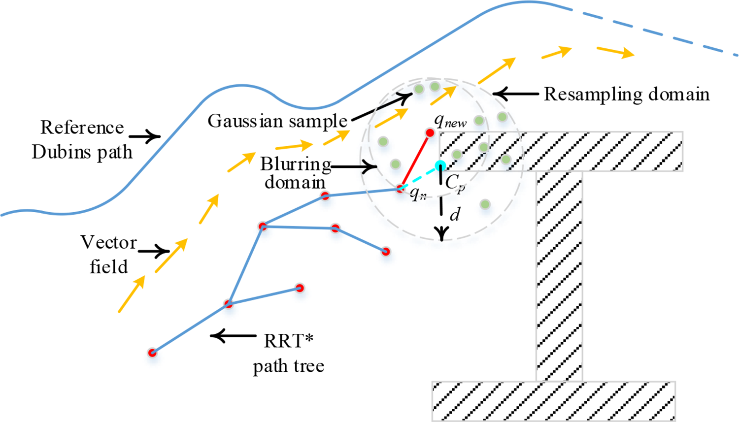
Illusion of the Gaussian sampling process.

During the extension from q_i to q_j , the expected direction of USV velocity coincides with the extension direction. To consider the current, the USV velocity is redefined as the resultant velocity of the originally expected USV velocity and the current velocity. Then, q_i is extended a step further on the direction of the resultant velocity.

The feasibility of the path is ensured since the path tree extends if the extension can pass the constraints checking. Once a local path is planned, the redundant waypoints are pruned from the path. The remained path is smoothed via Dubins curve.

Bounding box definition for collision avoidance

The accuracy of CD is important for the RRT-based methods, especially in the marine environment with the current. Thus, a bounding box is defined with the consideration of the USV velocity and the current velocity. The elliptic bounding box is used instead of a circular one to improve the OA efficiency of the planner because the USV body is asymmetrical.³¹

Figure 7 shows the elliptic bounding box for USV CD, and the USV body-fixed frame {b} shows the USV motion frame.

Figure 7.

Elliptic bounding box for USV collision detection. (a) Bounding box without consideration of the current and (b) bounding box considered the current. USV: unmanned surface vehicle.

Figure 7(a) shows the traditionally symmetrical bounding box without considering the current. The direction of the Y-axis of the {b}frame coincides with the USV velocity direction. The long axis of the elliptic bow bounding box is defined as L_b = L + ε_U + v Δt, where v is the velocity of USV, L is the length of USV, Δt is the duration of a control step, and ε_U is a positive value and we set it to be ε_U = 0.15 * v Δt, empirically.

When USV sails, the probability of USV suddenly turning back is tiny. Thus, we set the short axis of the bow bounding box to be W_b = W + ε_U , where W is the width of USV. The long axis of the stern bounding box is defined to be L_s = ε_U .

Figure 7(b) shows the asymmetrical bounding box with the consideration of current, and the direction of the Y-axis of the USV body-fixed frame does not coincide with the direction of the resultant velocity of the USV velocity and the current velocity. The bounding boxes of bow and stern on the left and right sides of USV are calculated separately. The long axis of the elliptic bow bounding box is defined as L_b = L + ε_U + max{v Δt + v_C * Δt sin θ_C , 0}, where v_C is the velocity of the current, and θ_C is the angle between the positive X-axis and the current direction, −π ≤ θ_C ≤ π. The short axis of the bow bounding box on the right side of USV is set to be W_b = W + max{ε_U + v_C * Δt cos θ_C , 0} and that on the left side of USV is set to be W_b = W + max{ε_U − v_C *·Δt cos θ_C , 0}. The long axis of the stern bounding box is defined to be L_s = max{−v_C *·Δt sin θ_C , 0} + ε_U .

Unmanned surface vehicles cooperative path planning

Suppose that USVs communicate in low power with each other and a member-only makes one-direction communication with a couple of members. Meanwhile, the computational ability of the ship-borne computer is limited. Thus, a distributed consensus-based cooperative strategy is applied to compute paths for USVs efficiently. The proposed heuristically sampling-based RRT* (HSRRT*) method is performed on the computer of the leader to an online plan for each state of the virtual leader, denoted by ξ^r = (x_c , y_c , θ_c ). (x_c , y_c , θ_c ) denotes the location and the velocity direction of the virtual leader. ξ^r is taken as the cooperation variable that is the minimum information that is communicated between USVs.

The communication between USVs can be modeled by a directed graph G = (V, E, A), where V = {1, 2,…, N} denotes the set of nodes with every node representing a USV. E ⊆ V × V denotes the set of communication edges of the USV formation systems. A = [a_ij ] ∈ R^N ^×N denotes a non-negative weighted adjacency matrix. Self-loops are excluded, that is, a_ii = 0. The edge e_ij = (i, j) ∈ E implies that USV _i (i = 1, 2,…, N) can receive information from USV _j (j = 1, 2,…, N).

The sketch map of the formation maintenance strategy is shown in Figure 8(a), where C ₀ is the inertial frame, C_Fi is the formation frame, and ξ_i = (x_ci , y_ci , θ_ci ) is the cooperative variable in the OPP system of USV _i . r_i = [x_i y_i ] and $r_{i}^{d} = [x_{i}^{d}, y_{i}^{d}]$ are the actual and expected positions of USV _i , and $r_{i F}^{d} = {[x_{i F}^{d}, y_{i F}^{d}]}^{T}$ is the expected deviation vector of USV _i relative to ξ_i

[\begin{array}{l} x_{i}^{d} (t) \\ y_{i}^{d} (t) \end{array}] = [\begin{array}{l} x_{c i} (t) \\ y_{c i} (t) \end{array}] + [\begin{matrix} cos [θ_{c i} (t)] & - sin [θ_{c i} (t)] \\ sin [θ_{c i} (t)] & cos [θ_{c i} (t)] \end{matrix}] [\begin{array}{l} x_{i F}^{d} (t) \\ y_{i F}^{d} (t) \end{array}]

Figure 8.

Sketch map of the cooperative paths planning for USVs. (a) Illustration of the formation maintenance and (b) cooperative paths planning framework. USV: unmanned surface vehicle.

To calculate paths for USVs, each member should have a consensus of the cooperative variable, that is, ξ^r = (x_c , y_c , θ_c ). The cooperative variable calculator of each USV is as follows

ξ_{i}' = \frac{1}{η_{i} (t)} \sum_{j = 1}^{n} a_{i j}^{c} (t) [ξ_{j}' - γ (ξ_{i} - ξ_{j})] + \frac{1}{η_{i} (t)} a_{i (n + 1)}^{c} (t) [ξ^{r}' - γ (ξ_{i} - ξ^{r})]

The virtual leader is regarded as the (n + 1)’th member, G_n+1 ^c denotes the communication topological model of the n + 1 members. $A_{n + 1}^{c} = [a_{i j}^{c}]$ is the adjacency matrix of communication, γ is a positive constant and it is set to be 0.3. $η_{i} (t) = \sum [a_{i j}^{c} (t)]$ , where j = 1…n + 1.

Figure 8(b) shows the framework of cooperative paths planning framework, and ξ_i denotes the cooperative variable calculated by USV _j and J_i (t) means the numbers of neighbors of USV _i in terms of cooperative variable consensus, N_i (t) means the numbers in terms of cooperative path planning. $r_{j}^{d}$ is calculated after ξ_j is obtained, and u_i is the computed cooperative strategy.

Assume that the dynamic system of the USV member is single integral, and $r_{i}' = u_{i}, i = 1, 2, ..., n$ . We apply the following cooperative path calculation algorithm

u_{i} = r_{i}^{d'} - α_{i} (r_{i} - r_{i}^{d}) - \sum_{j = 1}^{n +1} a_{i j}^{v} [(r_{i} - r_{i}^{d}) - (r_{j} - r_{j}^{d})]

where α_i is a positive constant and it is set as: α ₁ = 0.1, α ₂ = α ₃ = α ₄ = 0.3, and the adjacency matrix $G_{n}^{v}$ reflecting the communication topologic, and $a_{i j}^{v}$ is an item of $G_{n}^{v}$ using for transmitting the information of $r_{i} - r_{i}^{d}$ . $A_{n + 1}^{c} = [\begin{matrix} 0 & 0 & 0 & 0 & 1 \\ 1 & 0 & 0 & 1 & 0 \\ 0 & 1 & 0 & 0 & 0 \\ 1 & 0 & 1 & 0 & 0 \\ 0 & 0 & 0 & 0 & 0 \end{matrix}]$ and $A_{n}^{v} = [\begin{matrix} 0 & 1 & 1 & 0 \\ 1 & 0 & 0 & 1 \\ 0 & 1 & 0 & 0 \\ 1 & 0 & 1 & 0 \end{matrix}]$ . USVs can converge to the formation because $G_{n + 1}^{c}$ and $G_{n}^{v}$ have clusters of directed spanning trees.²⁰

Algorithm implementation

Algorithm 1 shows the implementation of the proposed HSRRT* method. Lines 5–16 are the OPP process. The path tree extends according to the vector field in the seventh line. Lines 10–12 show the path tree topological structure refining process by path tree rewiring, and the cost in the 11th line is the sum of Cdist values from the root of path tree to a tree node. The CD process in the 13th line is performed based on the bounding box of USV.

Algorithm 1

Online heuristic sampling-based RRT* algorithm.

Algorithms 2 and 3 are the Gaussian sampling-based and multisampling-based path tree extension schemes, respectively. The k_r in Algorithm 2 and the n_r in Algorithm 3 are equal to 9.

Algorithm 2

Gaussian sampling-based path tree extension.

Algorithm 3

Multisampling-based path tree extension.

Algorithm analysis

The RRT* scheme can spend O(log n) time in finding the near neighbors and spend log n log ^d m time in path tree extension in the environment with m obstacles under the path tree construction phase. Thus, the time complexity of RRT* in the processing phase is O(n log n log ^d m) in terms of basic operations, for example, addition, multiplication, and comparison, and n is the number of extension times.¹ RRT* spent O(n) time in searching for a minimum-cost path during the path query phase. The computational complexity of spawning an obstacle-free sample is much lower than that of the path extension. Thus, it can possibly improve the efficiency of RRT* by spawning multiple samples and selecting one that may contribute to the path-finding process by the extension of path tree near obstacles during the Gaussian sampling-based extension procedure. Meanwhile, the computational complexity of the multisampling-based path tree extension is similar to that of RRT*. Therefore, the path tree construction process of HSRRT* is possibly more efficient than that of RRT*.

During each path tree rewiring procedure, RRT* searches for the near neighbors (q _near) of a newly spawned sample q_s on the path tree within the distance r(card(V)) = min{γ _RRT * (log(card(V))/card(V))^1/d, η}, where “card” denotes the number of path tree nodes and η is the step length of the path tree extension. If γ _RRT* ≥ 2(1 + 1/d)^1/d (μ(χ _free)/ζ_d )^1/d, then RRT* is proven to be asymptotically optimal.¹ μ is the volume of the obstacle-free space, and ζ_d is the volume of the unit ball in the d-dimensional space. The radius of the resampling domain of HSRRT* is also set to be r(card(V)).

RRT* is probabilistically complete; thus, the decay rate of the failure probability is exponential under the assumption that the environment has good connectivity property, which can be guaranteed in most practical marine environments. Given that the heuristic sampling processes do not prevent RRT* from considering all potential low-cost paths as the planning time approaches infinity,^1,2 HSRRT* remains probabilistically complete and asymptotically optimal. The resulting paths of HSRRT* are feasible because the path tree expands on the basis of the motion model, and constraints are handled during the OPP process.

The global reference path is an optimal one under the known environmental information and the specific resolution. The OPP process of HSRRT* is guided by the reference path through the vector field within a probability threshold. The vector field, the cost distance function, and the heuristic sampling processes take the current into account. Meanwhile, the cost distance function considers the energy efficiency, path tortuosity, path collision probability, and path length. Thus, the path is possibly an energy-efficient, safe, and easy-to-execute one. As the biasing ratio through sampling reduction increases, the randomness in the exploration of the tree decreases because several samples are now used to refine the path in regions around tree nodes. A trade-off occurs between heuristic sampling rate and space exploration rate.

The bounding box definition considers the velocities of USV and the current, helping to improve the accuracy of the CD process compared to traditional bounding boxes.

Simulation results and analyses

Simulations are performed in a computer with Windows 10 64 bit OS, 16 G RAM, and Intel(R) Core(TM) i7-7820HQ CPU @ 2.90 GHz. The parameters of the USV dynamic model are shown in Table 1 according to the reference 30. Planning parameters are set in Table 2, where δ_c is the prediction time domain, δ_e is the control domain, PR is the radius of perception domain, Δt is the extending step duration, and γ _RRT* is used in a sample’s near neighbor searching process. The maximum speed of USV is 10 kn (5 m/s). The absolute value of the maximum translational acceleration is 1.5 m/s² and the maximum lateral acceleration is 10 m/s².

Table 1.

Parameters of the USV dynamic model.

m ₁₁ (kg)	m ₂₂ (kg)	m ₃₃ (kg × m²)	d_u (kg/s)	d_v (kg/s)	d_r (kg × m²/s)	B_u (m)
25.8	33.8	2.7	2	7	0.5	0.2

USV: unmanned surface vehicle.

Table 2.

Planning parameter setting.

δ_c (s)	δ_e (s)	PR (m)	Δt (s)	γ_RRT*
20	5	150	1	20

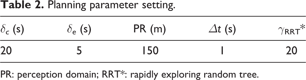
PR: perception domain; RRT*: rapidly exploring random tree.

Figure 9(a) and (b) shows the vector fields following linear and Dubins paths, respectively. Both fields take the current into account. The vector of a location in Figure 9(a) first finds the closest path segment, and then, the vector size and direction are computed. However, the linear path is not a practical one since it is not smooth with differential continuity and it does not consider the minimum turning radius of USV. Thus, the Dubins curve is used as the reference path, as shown in Figure 9(b). The vector calculation in Figure 9(b) is little complicated because arcs exist. Thus, the vector field is constructed by following the Dubins path. The current is taken into account in Figure 9(a) and (b).

Figure 9.

Vector field following reference paths and the current. (a) Vector field following the linear path and (b) vector field following the Dubins path with the consideration of the current.

Figure 10 shows the OPP results. The green curves show the global reference path while the red curves are the resulting paths in Figure 10(b) to (f). The elliptic function-based bounding boxes are shown at the turns on the resulting paths. The vectors in Figure 10(a) to (d) show the vector field with the consideration of the current. The green stars denote the subgoals. The start point is on the top left of the figure.

Figure 10.

Online path planning results for the virtual leader. (a) Path tree referring to the global path, (b) online planning result of HSRRT*, (c) planning result without Gaussian heuristics, (d) path without multisampling scheme, (e) planning result without following vector field, and (f) planning result of the RRT* method. RRT*: rapidly exploring random tree; HSRRT*: heuristically sampling-based rapidly exploring random tree.

Figure 10(a) shows the online generated path tree by HSRRT*, and the clustered lines consist of the path tree. In Figure 10(a), the red branches denote the vector following extensions and the blue branches denote the other heuristic extensions. Figure 10(b) shows an OPP result of the HSRRT* method. To certify the advantage of HSRRT*, results of other methods are shown. Figure 10(c) shows the planning result of the vector following multisampling RRT* (V-RRT*) method without the Gaussian sampling scheme. Figure 10(d) shows the result of the Gaussian function-based RRT* (Gaussian RRT*) method with vector field following mechanism but without multisampling mechanism. Figure 10(e) shows the planning result of the heuristic RRT* (HRRT*) method with Gaussian sampling and multisampling mechanism but without vector following mechanism. Figure 10(f) shows the result of the traditional RRT* method without heuristics.

The path tree in Figure 10(a) shows the path tree extension procedure of HSRRT*, and the vector following extensions guide the path returning to the reference path and handling the influence of the current. The randomness in path tree extensions is kept to find possible high quality paths. The randomness also prevents the planning from blocking by obstacles.

In Figure 10(b), the resulting path of HSRRT* deviates not far from the optimal reference path, demonstrating the low cost of the path, that is, mainly because of the vector field following scheme and the multisampling heuristic path tree extension. The path sections in the narrow passage on the right of figure have little turns, and the HSRRT* can find OA sections near obstacles, demonstrating the high collision-avoidance ability of HSRRT* probably because of the Gaussian sampling scheme. The path has many field-following sections, little counter-field sections and few transverse-field sections, demonstrating the effectiveness of the field following extensions. The path is possibly energy-efficient because of the consideration of the current in the vector field.

Figure 10(c) shows the result of planning without the Gaussian function-based heuristics. The path is zigzagged and deviates a little far from the reference path. Thus, the path is possibly more costly than that in Figure 10(b). However, the path follows the vector field well. The planner is less intended to search paths near obstacles than those related to Figure 10(b) and (d), resulting in less smooth sections with bigger turns in passages. The observation probably certifies the applicability of the Gaussian function-based sampling scheme.

Figure 10(d) shows the result of planning without the multisampling extension. The path is more zigzagged with more and bigger turns than those in Figure 10(b) and (c). The path has a bigger deviation from the reference path than that in Figure 10(b). The observation possibly testifies the effectiveness of the multisampling heuristics. Meanwhile, the path is smooth with less turns in the obstacle-dense passages on the right of the figure, comparing to that in Figure 10(c). That is possible because the planner can avoid obstacles by searching for paths near obstacle boundaries according to the Gaussian sampling-based extension scheme.

Figure 10(e) shows the path planned without the vector field following mechanism. The path deviates further from the reference path and is more different from the reference path. The path has more transverse vector field sections especially on the top right of the path. Meanwhile, the path is more zigzagged (with more and bigger turns) than those in Figure 10(b) to (d), especially on the top left of the figure, where big obstacle-free areas exist. Thus, the path in Figure 10(e) is probably more costly. The observations probably testify the applicability of the vector field-following heuristics. Figure 10(f) shows the planning result of RRT* without heuristics. The path is zigzagged (especially in passages) and deviates far from the reference path. The observation possibly certifies the lower path refinement efficiency and OA ability of RRT*. The observation also possibly demonstrates that RRT* converges slowly to the optimal path and the online planning time is limited.

The statistically numerical simulation results are provided in Table 3 related to Figure 10 to compare the methods. The data were collected after 1000 simulations were performed for each method. The average path searching time is denoted by “time.” The “time” is collected when the planner finds a path connecting the goal. The average path “cost” is computed by formula (6). The stabilities of algorithms are denoted by the standard deviations of time (time EVP) and cost (cost EVP).

Table 3.

Numerical simulation results.

Algorithm	Time (s)	Cost	Cost EVP	Time EVP	Cf(π)	FR
HSRRT*	1.1614	162.9760	3.6049	0.2359	0.8639	0.002
Gaussian-RRT* (no multisampling)	1.0743	176.9373	5.2133	0.3186	0.8010	0.002
V-RRT* (no Gaussian sampling)	1.4507	170.3487	8.0318	1.4050	0.8136	0.005
HRRT* (no vector following)	1.5778	180.8432	12.26	1.2299	0.7387	0.005
RRT*	4.5832	182.3739	13.3049	1.9562	0.5347	0.010

RRT*: rapidly exploring random tree; HRRT*: heuristic rapidly exploring random tree; HSRRT*: heuristically sampling-based rapidly exploring random tree; V-RRT*: vector rapidly exploring random tree; FR: failure rate.

The possible positions of USV at waypoint q_i are assumed to obey the n-variates normal distribution, thus, the lower bound of the collision-free probability of a path (π) with n waypoints is computed subject to $C f (π) = \prod_{i = 1}^{n} p_{c} (q_{i})$ and p_c obeys the standard Gamma distribution, p_c (q_i ) ≈ Γ(n/2, c_q ²/2), where c_q is the standard deviation of the USV positions that USV can collision-freely deviate from π and c_q = min{Dist _i } where Dist _i is the distance between USV and an obstacle. FR denotes the planning failure rate of local path searching processes.

The statistical values are used to demonstrate the performance of the HSRRT* method by comparing HSRRT* with traditional schemes.

The time value of HSRRT* is similar to those of Gaussian-RRT* and V-RRT* and much lower than those of HRRT* and RRT*, demonstrating the high efficiency of the vector field following the procedure of HSRRT*. The cost and cost estimated deviation of paths (EVP) of HSRRT* are lower than other methods, demonstrating the path of HSRRT* is more energy efficient and easy-to-execute with lower collision risk. That can also testify the high efficiency of HSRRT* because the online planning time is limited, thus, if the asymptotically optimal RRT* based method has higher efficiency, it possibly generates lower cost result. The Cf(π) and FR values of HSRRT* are the best. The above observations testify the effectiveness of the vector field and the environmental heuristics embedded into HSRRT*.

The cost and cost EVP of HSRRT* are better than those of Gaussian RRT*, demonstrating the applicability of the multisampling process. The time, time EVP, Cf(π), and FR values of HSRRT* are lower than those of V-RRT*, certifying the effectiveness of the Gaussian sampling.

The time, time EVP, Cf(π), and FR values of HSRRT* and Gaussian-based RRT* are better than that of V-RRT*, certifying the effectiveness of the Gaussian sampling in improving the obstacle avoiding ability of RRT*. Meanwhile, the better cost of V-RRT* than that of Gaussian-RRT* certifying that the multisampling process can improve the path refinement ability of RRT*. The cost EVP of Gaussian-RRT* is better than that of V-RRT*, possibly because that low-cost paths have smooth sections in passages in the experimental environment and the Gaussian-RRT* has stronger OA ability comparing to V-RRT*.

The performance indexes of HSRRT*, Gaussian-RRT*, V-RRT*, and HRRT* are much better than those of RRT*, demonstrating the applicability of the vector field and the proposed heuristics.

The cost of HRRT* is similar to that of RRT*, probably demonstrating the shape and length of the paths of HRRT* and RRT* are similar to each other. Thus, the Cf(π) values of HRRT* and RRT* are comparable. The bounding boxes used by HRRT* consider the current while those used by RRT* do not consider the current. The Cf(π) value of HRRT* is much better than that of RRT*, certifying the applicability of the proposed bounding box for CD.

Figure 11 shows the cooperative paths for USVs in a formation based on the information consistency and the virtual structure method, and the diamond formation helps to keep the communication links between USVs. In Figure 11(a), the green curve denotes the planned path for the virtual leader, and then, the members compute their cooperative paths to maintain the formation. The simulation in Figure 11(a) does not consider the OA problem. Figure 11(b) shows that USVs change the formation when passing passages because USVs cannot pass through passages in the diamond formation. The simulations testify that the proposed OPP method and cooperation scheme are applicable.

Figure 11.

Cooperative paths for USVs in a formation: (a) cooperative paths for formation maintaining and (b) cooperative paths with formation transformation. USV: unmanned surface vehicle.

Figure 12 shows the planning result on a hardware-in-the-loop platform. Figure 12(a) shows the current in a harbor. The current model can be regarded as time invariant in a short time and a small range. It is simulated as follows and it is generally clockwise in the northern hemisphere

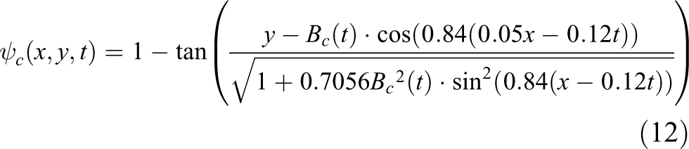
ψ_{c} (x, y, t) = 1 - tan (\frac{y - B_{c} (t) \cdot cos (0.84 (0.05 x - 0.12 t))}{\sqrt{1 + 0.7056 B_{c}^{2} (t) \cdot {sin}^{2} (0.84 (x - 0.12 t))}})

where the parameters are set empirically, B_c (t) = 1.2 + 0.3·cos(0.4·t +π/2). The velocity field of the current is also a vector field.

Figure 12.

Online path planning result on a hardware-in-the-loop platform. (a) Current in a harbor, (b) online planning result, and (c) 3D simulation of cooperative paths planning of USVs. USV: unmanned surface vehicle.

Figure 12(b) shows the OPP result, and the planning start point is shown by a red point. The green curve and the red curve are the reference path and the resulting path in Figure 12(b), respectively. The reference path is planned offline with the consideration of the current, thus, the reference path can generally follow the current. The current is also considered in the OPP process. The OPP result in Figure 12(b) has many downstream sections, thus, it is possibly energy efficient. That certifies the applicability and effectiveness of the proposed method with the consideration of the current. Figure 12(c) shows the three-dimensional simulation of cooperative path planning for USVs, and the right figure shows the cooperative paths when USVs change formation. Figure 12(a) to (d) shows simulation results of different systems, where the physical characteristics of USVs are simulated. The results demonstrate the effectiveness and practicability of the proposed HSRRT* method.

Conclusion

This article proposes a heuristically sampling-based random method to plan for energy-efficient, easy-to-execute, and low collision probability paths for USVs in the practical marine environment. The environment is modeled according to the vector field that follows the reference path and the current. Simulations certify that the vector field heuristics is applicable in improving the RRT*-based path planner. A Gaussian sampling-based path tree extension method is adopted, and it is proven to be effective in promoting the OA ability of the planner by extending to the samples near obstacles. A multisampling-based extension scheme is proposed and certified to be able to reduce the path cost. An elliptic bounding box is designed by considering the velocities of USV and the current, and results testify that the bounding box is applicable to decrease the collision probability of a path. Finally, an information consensus and virtual structure-based scheme is used to quickly calculate cooperative paths for USVs in a formation.

Supplemental material

Supplemental Material, ModificationTrace - Online planning low-cost paths for unmanned surface vehicles based on the artificial vector field and environmental heuristics

Supplemental Material, ModificationTrace for Online planning low-cost paths for unmanned surface vehicles based on the artificial vector field and environmental heuristics by Naifeng Wen, Rubo Zhang, Guanqun Liu, Junwei Wu and Xingru Qu in International Journal of Advanced Robotic Systems

Footnotes

Declaration of conflicting interests

The author(s) declared no potential conflicts of interest with respect to the research, authorship, and/or publication of this article.

Funding

The author(s) disclosed receipt of the following financial support for the research, authorship, and/or publication of this article: This work was supported in part by the National Natural Science Foundation of China [Grant No.61673084] and Key Laboratory of Intelligent Perception and Advanced Control of State Ethnic Affairs Commission [Grant No. MD-IPAC-2019103].

ORCID iD

Naifeng Wen

Supplemental material

Supplemental material for this article is available online.

References

Karaman

Frazzoli

. Sampling-based algorithms for optimal motion planning. Int J Robot Res 2011; 30: 846–894.

Jaillet

Cortés

Siméon

. Sampling-based path planning on configuration-space costmaps. IEEE Trans Robot 2010; 26: 635–646.

Boor

Overmars

Van Der Stappen

. The Gaussian sampling strategy for probabilistic roadmap planners. In: Proceedings 1999 IEEE international conference on robotics and automation (Cat No 99CH36288C), Detroit, Michigan, May 1999, pp. 1018–1023. New York, USA: IEEE Robotics and Automation Society.

Holland

McWilliams

. Computer modeling in physical oceanography from the global circulation to turbulence. Phys Today 1987; 40: 51–57.

Cao

Zhang

. Method of designing optimal smooth way for vehicle. J Syst Simul 2010; 22: 957–961.

Singh

Sharma

Sutton

, et al. A constrained A* approach towards optimal path planning for an unmanned surface vehicle in a maritime environment containing dynamic obstacles and ocean currents. Ocean Eng 2018; 169: 187–201.

Alvarez

Caiti

. A genetic algorithm for autonomous underwater vehicle route planning in ocean environments with complex space-time variability. IFAC Proc Volume 2001; 34: 237–242.

Soulignac

. Feasible and optimal path planning in strong current fields. IEEE Trans Robot 2010; 27: 89–98.

Niu

Savvaris

, et al. Energy efficient path planning for unmanned surface vehicle in spatially-temporally variant environment. Ocean Eng 2019; 196: 106766.

10.

Chi

, et al. A hybrid coordination controller for speed and heading control of underactuated unmanned surface vehicles system. Ocean Eng 2019; 176: 222–230.

11.

Garau

Bonet

Alvarez

, et al. Path planning for autonomous underwater vehicles in realistic oceanic current fields: application to gliders in the western mediterranean sea. J Mar Res 2009; 6: 5–22.

12.

Alvarez

Caiti

Onken

. Evolutionary path planning for autonomous underwater vehicles in a variable ocean. IEEE J Ocean Eng 2004; 29: 418–429.

13.

Garau

Alvarez

Oliver

. Path planning of autonomous underwater vehicles in current fields with complex spatial variability: an A* approach. In: Proceedings of the 2005 IEEE international conference on robotics and automation, Barcelona, Spain, 18–22 April 2005, pp. 194–198. New York, USA: IEEE Robotics and Automation Society.

14.

Lawrence

Frew

Pisano

. Lyapunov vector fields for autonomous unmanned aircraft flight control. J Guid Control Dyn 2008; 31: 1220–1229.

15.

Chen

Chang

Agate

. UAV path planning with tangent-plus-Lyapunov vector field guidance and obstacle avoidance. IEEE Trans Aerosp Electr Syst 2013; 49: 840–856.

16.

Owen

Nichols

Colton

. Cooperative aerial tracking and rendezvous along time-optimal 3-dimensional curves. In: AIAA guidance, navigation, and control conference, Portland, Oregon, 8–11 August 2011, p. 6546. New York, USA: AIAA.

17.

Gonçalves

Pimenta

Maia

, et al. Vector fields for robot navigation along time-varying curves in n-dimensions. IEEE Trans Robot 2010; 26: 647–659.

18.

Frew

Lawrence

Morris

. Coordinated standoff tracking of moving targets using Lyapunov guidance vector fields. J Guid Control Dyn 2008; 31: 290–306.

19.

Bibuli

Caharija

Pettersen

, et al. ILOS guidance-experiments and tuning. IFAC Proc Volume 2014; 47: 4209–4214.

20.

Ren

Beard

Atkins

. Information consensus in multivehicle cooperative control. IEEE Control Syst Mag 2007; 27: 71–82.

21.

M-Y

Wang

D-S

Wang

C-L

. Formation control for water-jet USV based on bio-inspired method. China Ocean Eng 2018; 32: 117–122.

22.

Qin

Lin

Yang

, et al. A task-based hierarchical control strategy for autonomous motion of an unmanned surface vehicle swarm. Appl Ocean Res 2017; 65: 251–261.

23.

Casalino

Turetta

Simetti

. A three-layered architecture for real time path planning and obstacle avoidance for surveillance USVs operating in harbour fields. In: Oceans 2009-Europe, Bremen, Germany, 11–14 May 2009, pp. 1–8. Bremen, Germany: IEEE Oceanic Engineering Society.

24.

Liang

Wang

, et al. Swarm control with collision avoidance for multiple underactuated surface vehicles. Ocean Eng 2019; 191: 106516.

25.

Liang

Wang

, et al. A novel distributed and self-organized swarm control framework for underactuated unmanned marine vehicles. IEEE Access 2019; 7: 112703–112712.

26.

Wang

Xie

Pan

, et al. Full-state regulation control of asymmetric underactuated surface vehicles. IEEE Trans Ind Electron 2019; 66: 8741–8750.

27.

Wang

S-F

Pan

, et al. Yaw-guided trajectory tracking control of an asymmetric underactuated surface vehicle. IEEE Trans Ind Inform 2019; 15: 3502–3513.

28.

Wang

Karimi

, et al. Accurate trajectory tracking of disturbed surface vehicles: a finite-time control approach. IEEE/ASME Trans Mechatron 2019; 24: 1064–1074.

29.

Motus

. Time concepts in real-time software. Control Eng Pract 1993; 1: 21–33.

30.

Mousazadeh

Kiapey

AJCOE

. Experimental evaluation of a new developed algorithm for an autonomous surface vehicle and comparison with simulink results. China Ocean Eng 2019; 33: 268–278.

31.

Tam

Richard

. Collision risk assessment for ships. J Mar Sci Technol 2010; 15: 257–270.

Supplementary Material

Please find the following supplemental material available below.

For Open Access articles published under a Creative Commons License, all supplemental material carries the same license as the article it is associated with.

For non-Open Access articles published, all supplemental material carries a non-exclusive license, and permission requests for re-use of supplemental material or any part of supplemental material shall be sent directly to the copyright owner as specified in the copyright notice associated with the article.

0.00 MB

0.96 MB