Sage Journals: Discover world-class research

Abstract

China has been the world’s largest automotive manufacturing country since 2008. The automotive wheel industry in China has been growing steadily in pace with the automobile industry. Visual recognition system that automatically classifies wheel types is a key component in the wheel production line. Traditional recognition methods are mainly based on extracted feature matching. Their accuracy, robustness, and processing speed are often compromised considerably in actual production. To overcome this problem, we proposed a convolutional neural network approach to adaptively classify wheel types in actual production lines with a complex visual background. The essential steps to achieve wheel identification include image acquisition, image preprocessing, and classification. The image differencing algorithm and histogram technique are developed on acquired wheel images to remove track disturbances. The wheel images after image processing were organized into training and test sets. This approach improved the residual network model ResNet-18 and then evaluated this model based on the wheel test data. Experiments showed that this method can obtain an accuracy over 98% on nearly 70,000 wheel images and its single image processing time can reach millisecond level.

Keywords

Wheel production manufacturing image recognition convolutional neural network digital image processing

Introduction

With the rapid technological development nowadays, manufacturing is becoming less labor-intensive and more capable of intelligently adapting to a variety of changing conditions. China has been the world’s largest automotive manufacturing country since 2008. The demand for automobile wheel production is therefore enormous. As a key component in the manufacturing system, wheel production line’s level of automation is of great significance and economic value. During the production, a variety of wheels are sent to the conveyor belt after the stage of low-pressure casting. These wheels are required to be classified before going through different machining processes. The visual recognition system that classifies these wheels is an essential element to achieve multi-varietal mixed-flow production in automated production lines.

As shown in Figure 1, wheel parameters usually consist of thread holes, spoke windows, gas nozzles, and the outer circle size. These characteristics of the wheel parameters provided in this scheme are mainly the characteristic parameters required for further processing based on the entire wheel structure. These geometric parameters include wheel radius, area, perimeter, number of spoke windows, and number of internal bolt holes. And Figure 1 illustrates the principle of the entire identification system. Firstly, the programmable logic controller (PLC) controls the camera to collect various wheel images on the production line to build a wheel database. Then we build a wheel recognition system based on the image recognition algorithm and the collected wheel database to identify the wheels flowing on the production line.

Figure 1.

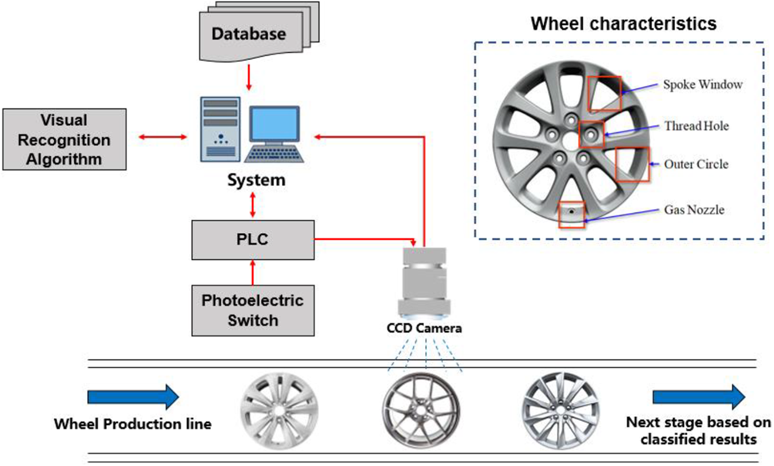
Visual recognition system to classify wheel types and wheel characteristics.

For traditional image identification methods, the acquisition of the above feature parameters (artificial features) is of great significance to the subsequent processing and identification of the wheel. Researchers have attempted to apply digital image processing technology to this field. Zhao and Liu^1,2 segmented the background based on the gray histogram technique, effectively eliminating the interference background and ensuring the complete extraction of the wheel. They extracted four ideal features of the wheel and achieved a 99% wheel recognition rate based on the voting classifier. However, this background interference and the wheel feature parameters extraction are relatively simple. And the number and types of test images are relatively small. Cheng et al.³ proposed the automobile wheel model identification based on the shape recognition and texture filtering algorithm. They tested the effectiveness of the algorithm based on 120 images of five wheel types. However, the algorithm does not have a high recognition rate for the wheel with complex textures especially when there are a lot of burrs on the wheel. Zhu et al.⁴ extracted seven features with rotational invariance on the wheel and implemented efficient wheel identification based on the digital sequence method. However, this recognition method still uses artificial features to identify without taking the complex wheel production line background interference into account. Guo et al.⁵ characterize the shape of various types of wheels by extracting constants with rotational invariance such as the number of spokes, the diameter of the center hole, and the area ratio of the perimeter of the web. Finally, a serial number is generated for the extracted feature parameters for wheel identification. In summary, these researchers are trying to apply traditional image recognition to simple industrial vision problems. With the rise of industrial big data,⁶ the limitations of traditional machine vision make deep learning⁷ technology gradually applied to industrial production scenarios. Deep learning technology represented by convolutional neural network (CNN)⁸ shines in the field of image recognition. Cheng and Zhou⁹ proposed a character recognition method based on improved CNN. Experimental results show that the training accuracy of this method is over 99% and the recognition accuracy is 98.5%. Deng and Wang¹⁰ aimed at the problem of vehicle identification in highway environment. The theory of CNN is introduced and the corresponding feature extraction algorithm is designed. The identification system is constructed by combining support vector machine (SVM) classifier.¹¹ CNN technology is more and more widely used in industrial image recognition.¹² It is foreseeable that CNN will replace the ancient artificial features of image recognition methods in the field of industrial image recognition.

Image recognition technology can be divided into traditional wheel recognition methods and deep learning-based image recognition methods according to feature extraction methods.^2,13

-16 The difference between the traditional identification method and the deep learning method is shown in Figure 2. Take the wheel identification problem for example, the traditional identification wheel method relies on the artificial features analysis of the image to match the category of the wheel, such as geometric features and texture features, while the network adaptive feature of deep learning can identify the wheel by autonomous feature learning, thus avoiding the design of artificial features. It is obvious that the latter has better reliability and robustness. To overcome the drawbacks of traditional image identification methods, we proposed a CNN approach to adaptively classify wheel types in actual production lines with a complex visual background. The aim of this work is to obtain better quality and less interference images. Through the CNN method, we can effectively realize the fine-grained image recognition task without artificial features that are difficult to extract.

Figure 2.

The difference between the traditional identification method and deep learning method.

To release the difficulty of model training, the contribution of this article is to use the traditional image processing techniques to complete the extraction and denoising of the central area of the original wheel image. The core of the recognition algorithm is to build a lightweight residual network model based on deep learning technology to realize the identification of wheel types. Experiments show that this model can solve the difficulty of identifying wheels with large burr and low recognition speed that cannot be solved by traditional recognition methods. Specifically, the model can achieve a recognition accuracy of more than 98% on nearly 70,000 images and a recognition speed of milliseconds.

Methodology

This study proposed an image recognition method for wheel identification based on CNN, which mainly include image acquisition, image preprocessing, design the network model, define the loss function, and batch gradient descent algorithm. The specific operation process is shown in Figure 3. The main idea was to preprocess industrially acquired wheel images through classic image processing methods to obtain wheel’s region of interest. The specific preprocessing process mainly consists of three algorithms: improved image difference algorithm, edge extraction and image segmentation, and median filtering. This method is good for improving the processing time and accuracy of existing CNN network to classify wheel images.

Figure 3.

Image recognition flowchart.

Image acquisition and preprocessing

Nearly 70,000 wheel pictures that consist of 19 wheel types were collected through our self-built image acquisition system. As shown in Figure 1, the existing wheel image acquisition device mainly includes industrial camera (Japanese Omron industrial grade CCD camera with 2-megapixel resolution), LED fixed light sources, image acquisition card, and industrial computer. The wheel was placed on the conveyor belt at random orders. A reasonable image analysis and appropriate image processing method is a key step after image acquisition. Combined with the acquired background and wheel images (Figure 4(a) and (b)), the analysis of the acquired image is summarized as follows. The strong reflection of the conveyor belt to the light source and the faintly visible bracket below the conveyor belt were strong disturbances which affected the accurate extraction of the parameters of the wheel. The brightness between the conveyor belts was different from the original due to the random placement of the wheel and the blocking of the light. The roller randomly passed through the spoke window of the wheel and sometimes even filled the entire spoke window, interfering with counting the number of spokes. There were a large number of burrs in the wheel blank before machining and the center hole and the threaded hole were not drilled, which affected counting the number of threaded holes.

Figure 4.

(a) The shining surface of the roller and (b) image of wheel visually contaminated by the conveyor belt.

In order to realize the recognition of the wheel, the above problems must be solved. Image analysis showed that traditional methods based on artificial feature extraction and recognition were difficult to implement in this complex industrial background. However, if the captured image is directly used for CNN training, it will easily fall into over-fitting¹⁷ due to too many irrelevant features. A better method is to remove most of the conveyor belt by image processing to reduce the training pressure of the CNN.

Due to the influence of hardware and lighting, there was often a lot of noise in the collected wheel images. Image preprocessing technology eliminated image noise and made subsequent image processing results more accurate. Image preprocessing technology mainly includes grayscale transformation¹⁸ of image and Gaussian filtering¹⁹ noise reduction which must be performed before image recognition work. The purpose of image grayscale²⁰ was to convert the acquired image into an 8-bit single-channel image format which is beneficial for simplifying the entire image processing work. Gaussian filter noise reduction technology is the most commonly used image denoising method. Since the subsequent image processing technology involves image detail parts such as edge extraction,²¹ the presence of noise will produce a large error in subsequent processing and achieving the expected effect may not be possible.

Improved image differencing

Through the improved image differencing algorithm, we removed the conveyor belt outside the wheel as much as possible to reduce the amount of image processing data. From the perspective of reducing the number of features of the data, this approach was effective in improving the learning ability of CNN model. The gray histogram is a function of the gray level of the image and it is used to count the number of pixels or the occupancy of each gray level in the image array.²² In this study, the histogram technique was primarily used to analyze the pixel interval in which the interference factor is located, combining the image difference method to reduce the non-primary region in the image quantitatively.²³ Since the wheel was in a region of high brightness, based on the histogram, most of the main characteristic pixels of the wheel were concentrated on the left peak of the histogram. And the tail on the right was the bracket interference under the conveyor belt. By selecting the appropriate luminance as the image threshold, the wheel image was segmented by threshold segmentation.²⁴

To achieve the complete separation of the wheel and conveyor belts, an image differencing algorithm which is widely used in video analysis²⁵ was required. The specific principle is as follows

\begin{array}{l} O (r, c) = I {(r, c)}_{wheel} - I {(r, c)}_{bground} \\ 0 \leq r \leq H - 1, 0 \leq c \leq W - 1 \end{array}

where the wheel image height is H, and width is W. Among them, $I {(r, c)}_{wheel}$ is the acquisition image of the wheel, $I {(r, c)}_{bground}$ is the acquired image of the complex background, and $O (r, c)$ is the output image difference image. The specific method is to collect the background image without the wheel from the previous moment and the image containing the conveyor belt and the wheel at the next moment. The two images were then subjected to different calculations, allowing the conveyor belt to be substantially separated from the wheel image. Such a treatment method is not affected by the random placement of the wheel. Based on the above analysis, the specific algorithm steps are as follows:

(1) Collect the wheel image $I {(r, c)}_{wheel}$ and the corresponding background image $I {(r, c)}_{bground}$ as the input image.

(2) Calculate the gray histogram $I {(r, c)}_{bground}$ of the wheel image $I {(r, c)}_{wheel}$ and determine the threshold value c ₀ (the threshold value is 40 in this case) based on the gray histogram analysis.

(3) Traverse the wheel image $I {(r, c)}_{wheel}$ and the background image $I {(r, c)}_{bground}$ of each pixel value, above the threshold c ₀ is retained, otherwise set to 0 (0 means black), respectively, and obtain the image $I^{'} {(r, c)}_{wheel}$ and $I^{'} {(r, c)}_{bground}$

I^{'} {(r, c)}_{wheel} = \{\begin{matrix} I {(r, c)}_{wheel} I {(r, c)}_{wheel} > c_{0} \\ 0 I {(r, c)}_{wheel} > c_{0} \end{matrix}

I^{'} {(r, c)}_{bground} = \{\begin{matrix} I {(r, c)}_{bground} I {(r, c)}_{bground} > c_{0} \\ 0 I {(r, c)}_{bground} > c_{0} \end{matrix}

(4) Calculate the output image based on the image difference algorithm between $I^{'} {(r, c)}_{wheel}$ and $I^{'} {(r, c)}_{bground}$

\begin{array}{l} O (r, c) = I^{'} {(r, c)}_{wheel} - I^{'} {(r, c)}_{bground} \\ 0 \leq r \leq H - 1, 0 \leq c \leq W - 1 \end{array}

The image differencing method was indeed effective in removing most of the conveyor belts outside the wheel, but this process inevitably caused damage to the entire wheel image. A median filtering algorithm was used to repair the damaged part of the wheel which is beneficial to the complete acquisition of the entire wheel surface. Median filtering technique²⁶ is a neighborhood operation based on sorting statistics theory. This filtering method selects the median value in the group as the gray value of the output so that the surrounding pixel values are close to the true value, thereby eliminating the isolated noise points.²⁷ At the same time, the choice of the radius of the filter kernel window²⁸ plays a key role in the restoration of the wheel image. In general, the choice of window size depends mainly on the size of the interference area in the image. The pixel areas smaller than the window radius will be filtered out and the target larger than the window radius will be retained.

Edge detection and image segmentation

After median filtering, we used edge detection and the geometric method of the smallest circumscribed circle to strip most of the conveyor belts from the wheel image to ensure that the pixels of the wheel surface in the image account for the vast majority. This part includes Canny edge detection algorithm,²⁹ the theory of which can be seen in Figure 5, synthesizing these edge pixels and the minimum circumscribed circle fitting algorithm. In Figure 5, it is noted that “sobelx” represents a Sobel convolution template in the x-direction, “sobely” represents a Sobel convolution template in the y-direction, “*” represents convolution calculation, “magnitude” and “angle” represent the image gradient and the corresponding gradient direction respectively. Canny edge detection mainly consists of three steps: image gradient calculation, non-maximum suppression, and dual threshold lag processing. The image gradient calculation mainly uses the convolution of the Sobel operator³⁰ with the image to obtain the x-direction gradient “dx” and the y-direction gradient “dy” of the image. Non-maximum suppression was mainly used to preserve the maximum value in the gradient direction and discard the non-maximum value. The double threshold lag processing mainly determined whether to retain the pixel points between the high and low thresholds in the gradient image.

Figure 5.

Canny edge extraction and image segmentation flowchart.

Different from edge detection algorithms based on convolution operations such as Sobel and Prewitt,³¹ the Canny edge detection algorithm fully considers the gradient direction of image edges and proposes a non-maximum suppression strategy based on edge gradient direction and a double threshold hysteresis threshold processing method. In this scheme, the Canny edge detection algorithm can be also used to detect the pixels of the contour boundary according to the difference between pixels. The next step is to synthesize these edge pixels which will benefit the contour statistics.³² This algorithm has been able to directly implement the synthesis and counting of contours in open source computer vision library (OpenCV), based on the “findContours” algorithm.³³ Then filtering the outline should be required. The specific method is to calculate the area inside the contour, as is known, the contour which has largest area is the maximum contour, that is, the outer circle of the wheel. In order to make up for the above shortcomings, this scheme adopts the minimum circumscribed circle fitting algorithm,³³ that is, traversing the points of all connected regions, finding the four outermost points to generate a circle, judging whether other points are in the circle and adjusting the center of the circle based on the judgment result and size until a circle is found that contains all of the connected points. Another advantage of this function is the ability to acquire the center and radius of this smallest circumscribed circle in time. Based on the above analysis, the specific algorithm flow is summarized. First, the Canny operator was used for edge detection. Contour detection and discovery was based on “findContours” algorithm. Next, all contours were traversed and sorted by area and the contour with the largest area was extracted. Lastly, the contour extracted in the previous step was applied with a minimum circumscribed circle fitting algorithm.

CNN network model design

Based on the image processing discussed before, most of the conveyor belts were removed, which is beneficial to the effective recognition of the subsequent steps from the perspective of feature dimension reduction. Moreover, it was difficult to completely remove the conveyor belt to retain only the entire wheel and this did not make sense because the feature combination of the CNN was powerful enough to suppress these small disturbances. This part mainly discussed the method of designing the CNN model.

CNN models were designed based on the ImageNet data set³⁴ such as VGG,³⁵ NIN,³⁶ GoogLeNet,³⁷ and ResNet.³⁸ These models are powerful enough to fit data sets with millions of data volumes. But it was challenging to apply these models in real-world industrial scenarios. For example, in the wheel production line, we only collected less than 70,000 images through the front end. If applying the above existing models directly, unless using the migration learning method,³⁹ we would inevitably encounter severe over-fitting. Here we did not use migration learning and designed a CNN suitable for small data sets in the industrial field based on the residual network and other basic layers of CNNs. These basic layers mainly include a fully connected (FC) layer, an active layer, a convolution layer, a batch normalization layer, a discard layer, and a pooling layer. The FC layer, as the name implies, connected all the input nodes and output nodes and finally realized the linear operation. For the activation layer, this article mainly used the Relu function as the activation layer and its expression is as follows

relu (x) = \{\begin{matrix} x x > 0 \\ 0 x \leq 0 \end{matrix}

The main role of this layer was to nonlinearly map the input nodes, thereby improving the nonlinear representation of the neural network. The convolutional layer is the most characteristic level in the CNN. The CNN mainly realizes the combination of multiple pixels around by convolution operation, which can further extract the features in the image and reflect the powerful feature engineering ability inside the network. The pooling layer is similar to the convolutional layer and is often divided into a maximum pooling layer and an average pooling layer. The largest pooling layer mainly returns the maximum value in the pixel region among them. This type of pooling layer can reduce the width and height of the image, effectively reducing the risk of model over-fitting. The discard layer is based on the threshold preset by the designer and randomly discards the output unit of the upper layer with the threshold probability.

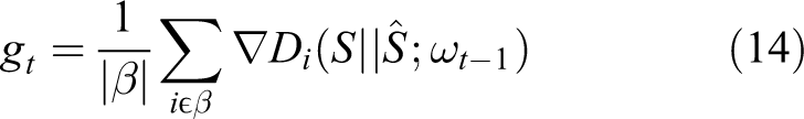
For the batch normalization layer, the normalization of a single sample was mainly achieved on small batch samples. Its main role was to adjust the intermediate output of the neural network, which is beneficial to reduce the instability of the numerical calculation in the model. The principle of batch normalization is relatively simple. For any sample xⁱ , $1 \leq i \leq m$ in a small batch $β = \{x^{1}, x^{2}, \dots, x^{m}\}$ , we can calculate the mean $μ_{β}$ and variance $σ_{β}^{2}$ of this batch β by the following formula

μ_{β} = \frac{1}{m} \sum_{i = 1}^{m} x^{i}

σ_{β}^{2} = \frac{1}{m} \sum_{i = 1}^{m} {(x^{i} - μ_{β})}^{2}

After deriving the mean and variance, we can standardize the sample xⁱ as ${\hat{x}}^{i}$

{\hat{x}}^{i} = \frac{x^{i} - μ_{β}}{\sqrt{σ_{β}^{2} + ε}}

The ε in the denominator is to prevent the numerical calculation overflow caused by the variance of 0.

Finally, by learning the stretching parameters γ and offset parameters ρ, as in equation (9), construct a batch normalized output $x_{out}^{i}$

x_{out}^{i} = γ \cdot {\hat{x}}^{i} + ρ

In addition to the above basic layer, the network designed in this article also has the most important module, that is, residual module. The residual module is derived from the residual network model ResNet. The idea of the ResNet model is to make the data forward faster by adopting the cross-layer connection design, so as to solve the problem of increased error on the training set caused by the much deeper network. ResNet thus introduced the residual block shown in Figure 6.

Figure 6.

The principle of residual model.

Assuming that the input of a certain neural network is x, the expected output is H(x) and H(x) is the expected complex potential mapping. In the residual network structure diagram of Figure 6, the input x is directly transmitted to the output as an initial result by means of “shortcut connections” and the output result is H(x) = F(x) + x. When F(x) = 0, then H(x) = x, that is, the expected output is an identity map. Thus, ResNet is equivalent to changing the learning target to the difference between the learning target value H(x) and x, which is the so-called residual F(x) = H(x) − x. Therefore, the latter training goal is to approximate the residual result to 0, so that the accuracy does not decrease as the network deepens.

The smallest model of residual network design in the original text is ResNet-18.⁴⁰ ResNet-18 follows the first two layers of GoogLeNet: a 5 × 5 convolutional layer with 16 output channels and 2 strides, followed by a 3 × 3 maximum pooling layer with 2 strides. Then it connected four basic modules composed of residual blocks and the residual block in each module multiplies the number of channels of the previous module. Finally, after the global average pooling layer, the FC layer was connected.

The CNN model designed in this study was based on this residual module. Since there were only 10 layers of convolutional layers, we used ResNet-10 instead of the deep learning model designed. The first two layers of ResNet-10 draw on the design of ResNet-18, only changing the number of output channels and the size of the convolution kernel: the 5 × 5 convolutional layer with 16 output channels and 2 steps is followed by the 3 × 3 maximum pooling layer of with 2 strides. However, ResNet-10 uses two kind of modules: one is residual blocks with an output channel number of 16 and the other is residual blocks with an output channel number of 32. Unlike ResNet-18, the two residual modules are not directly connected. Instead, the output of the first residual module is batch normalized and then through a maximum pooling layer and a discarding layer. The main purpose was to effectively avoid over-fitting while deepening the network. The last two layers are designed in the same way as ResNet-18, with the global pooling layer and the full connection layer directly outputting the category. The advantage of designing a model like this is that instead of simplifying the model, it provides a way to simplify the existing model, which is to keep the model deep enough while simplifying the model. Because the development of deep learning shows that neural networks that are deep enough are often more effective for image recognition tasks than shallow neural networks. The overall model architecture of ResNet-10 can be found in Figure 7. It is noted that “Conv” refers to the convolution layer, “Batch Norm” refers to the batch normalization layer, “Activation” refers to the active layer, “Max pool” and “Avg Pool” refer to the pooling layer, “Dropout” refers to the discard layer, and “FC” refers to fully connected layer.

Figure 7.

The structure of residual model 10.

Loss function and batch gradient descent algorithm

After the model was established, an evaluation function was defined to evaluate the parameters of the model and an optimization algorithm was used to optimize the model based on the evaluation results. The loss function was used to estimate the degree of inconsistency between the prediction category $f (x; θ)$ of the model and the real category y of the sample. It is a non-negative function, usually the smaller the loss function, the better the robustness of the model. The loss function is also an important part of the structural risk function. In general, the structural risk function of a model with θ as a parameter includes the empirical risk term $L (y_{i}, f (x_{i}; θ))$ and the regular term $Φ (θ) .$ ⁴¹ Usually it can be expressed as follows

θ^{*} = arg min_{θ} \frac{1}{N} \sum_{i = 1}^{N} L (y_{i}, f (x_{i}; θ)) + λ Φ (θ)

where i denotes the ith sample, N denotes the total number of samples, λ denotes a penalty parameter, and a larger λ means that the complexity limit of the model is larger.

The loss function selected in the ResNet-10 model is the cross entropy function commonly used for classification and the regularization method uses the weight decay method.⁴² The intensity of weight attenuation depends mainly on the weight attenuation coefficient. For the 19 types of wheels involved in this article, the cross entropy function is derived by taking a single sample as an example. The CNN can effectively predict the category according to the image features and the essence is to predict the probability distribution⁴³ that the category satisfies. Let us set the true probability distribution of the 19 categories of the wheel as $S = (s_{1}, s_{2}, \dots, s_{19})$ , where let $s_{k} (k = 1, 2, 3, \dots, 19)$ denote the true probability that the image sample y belongs to the kth class. While the CNN gives the predicted distribution as $\hat{S} = ({\hat{s}}_{1}, {\hat{s}}_{2}, {\hat{s}}_{3}, \dots, {\hat{s}}_{19})$ , where ${\hat{s}}_{k} (k = 1, 2, 3, \dots, 19)$ represents the prediction probability of the image sample y belonging to the kth class. Based on the one-hot coding⁴⁴ of the true probability distribution, when the sample S belongs to the kth class, there must be $s_{k} = 1$ and all other components are 0, indicating that the other classes belong to a probability of 0. Based on knowledge of probability theory and information theory, we can use KL divergence⁴⁵ to measure the difference between two probability distributions. Corresponding to any probability event $x \in X$ , the known probability distributions P(x) and Q(x), their KL divergence formula is as follows

D (P | | Q) = \sum_{x \in X} P (x) \cdot log \frac{P (x)}{Q (x)}

The true probability distribution S and the predicted distribution $\hat{S}$ were substituted into the above formula

D (S | | \hat{S}) = \sum_{x \in X} S (x) \cdot log \frac{S (x)}{\hat{S} (x)} = \sum_{i = 1}^{19} s_{i} \cdot log \frac{s_{i}}{{\hat{s}}_{i}}

When the image sample y belongs to the kth class

D (S | | \hat{S}) = \sum_{i = 1}^{19} s_{i} \cdot log \frac{s_{i}}{{\hat{s}}_{i}} = - log s_{k}

The above formula is the expression of the cross entropy function, which is also the concrete form of the loss function in the CNN. By defining the loss function, the difference between the true probability distribution and the predicted probability distribution can be well measured. In the following, only the parameter ω in the network needs to be updated by the backpropagation algorithm⁴⁶ according to the difference. 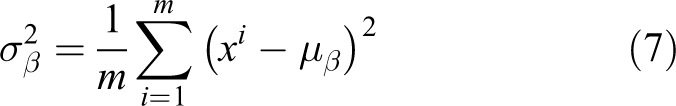One of the more important steps in the backpropagation algorithm is the choice of the gradient optimization method.⁴⁷ In this article, the small batch gradient descent method is mainly used, that is, the gradient g_t for $ω_{t - 1}$ at the loss function $D (S | | \hat{S})$ of the time step t is calculated on the small batch sample β. Update ω as follows

g_{t} = \frac{1}{|β|} \sum_{i ϵ β} \nabla D_{i} (S | | \hat{S}; ω_{t - 1})

ω_{t} = ω_{t - 1} - η \cdot g_{t}

where |β| represents the total number of samples of the small batch sample β, $\nabla D_{i} (S | | \hat{S}; ω_{t - 1})$ represents the gradient of the parameter $ω_{t - 1}$ at the loss function $D (S | | \hat{S})$ on the ith sample, and η is the learning rate which is between 0 and 1. So far, we have explained the main technical principles of CNN design.

Finally, we mainly preprocessed 70,000 images with 19 wheel categories collected at the front end based on the above image processing method. The purpose of the pretreatment was to primarily separate the wheel from the background of the production line. The processed wheel picture was then split into 80% as a training set for training the above CNN ResNet-10 and the remaining 20% is used as a test set to verify the model accuracy. Specifically, it was divided into four major steps. These steps include wheel images acquisition, traditional image processing for achieving the segmentation of the wheel, training ResNet-10, and verifying the model accuracy, as shown in Figure 8. The more detailed hyperparametric design part is detailed in the third part of this article.

Figure 8.

Program flowchart.

Result and discussion

Results of image separation in a complex background

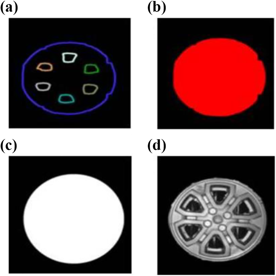
In this part, we used one of the wheels as an example to illustrate the effectiveness of traditional image processing methods for wheel segmentation. After image preprocessing and improved image differencing algorithm, the wheel image was damaged which needs to be repaired properly, as shown in Figure 9(b). The goal was to retain the maximum outer circle of the wheel. To simplify the image processing method, a threshold separation method was developed to fill unnecessary holes in the wheel, which is based on histogram technique. Taking the black stripes appearing in Figure 4 into consideration, we selected a suitable filter kernel based on the median filtering method.

Figure 9.

Achieving the segmentation of the wheel: (a) image preprocessing including grayscale transformation and Gaussian filtering, (b) improved image difference algorithm, (c) threshold operation,⁴⁸ and (d) median filtering method for filling tiny holes.

In this scheme, the median filter core with a radius of 17 was selected and the tiny holes in the wheel were filled by applying the opening and closing operation in the morphological operation.⁴⁹ As shown in Figure 9(d), the complicated production line background of the wheel was completely eliminated and the opening and closing operation ensured that the geometrical characteristics such as the wheel area did not change greatly. At the same time, the continuity of the maximum contour of the wheel ensured the effectiveness of subsequent edge extraction.

The wheel contour was clearly visible based on the image of the wheel. Therefore, we obtained all the contours of the wheel in OpenCV (Figure 10(b)). The maximum contour was founded using the maximum contour screening method (refer to the “Edge detection and image segmentation” section). To accurately obtain the outer circle of the wheel and fill in the contour defects, the largest outer circle was acquired by the minimum circle fitting algorithm. In Figure 10(c), the outer circle is marked in white. Finally, we performed the AND operation⁵⁰ on the original image containing the production line and the processed image to get the whole wheel.

Figure 10.

Spoke number extraction and geometry measurement: (a) Canny edge detection for wheel; (b) find the maximum contour based on the find contours algorithm; (c) contour minimum circumscribed circle fitting of the largest; (d) AND operation to get the whole wheel.

Figure 11 shows the image separation results of the other 18 wheel types. The conveyor belt in the processed image was nearly unnoticeable. Although there were large burrs at wheel surface which posed challenges to traditional identification methods, this did not affect the performance of the deep learning approach.

Figure 11.

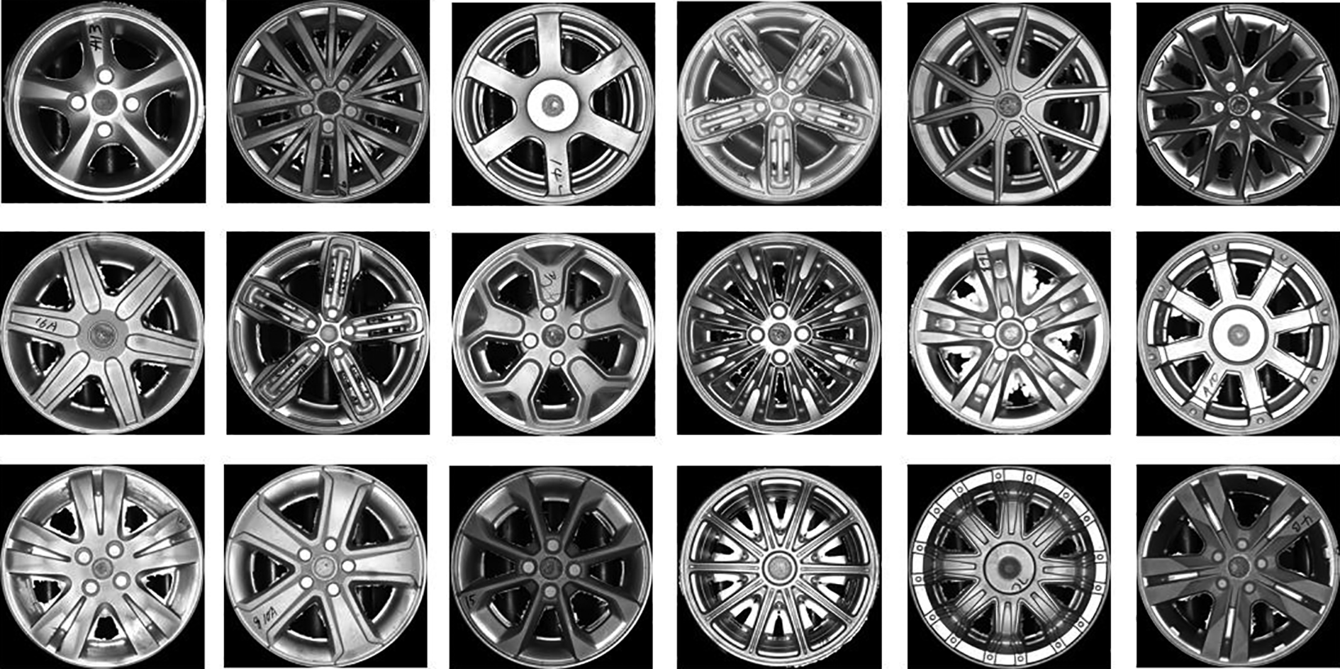
The other 18 separated wheel types (conveyor belt removed).

Results of visual recognition method

This section covers the training details of the model ResNet-10, in order to verify that the model can classify the above 19 wheel types with high accuracy. Its main idea was that by designing the CNN model’s parameters,⁵¹ we calculated the loss value in each iteration on the training set. We then gave the correct rate of the model on the training set and the test set. The parameters in the CNN model include the number of steps in which the model parameters are iteratively updated, the learning rate of the small batch gradient algorithm, the batch size of the single training, weight attenuation coefficient, and the size of the input image data. The specific parameter design values are shown in Table 1. These parameter values were repeatedly adjusted in order to improve the generalizability of the designed CNN.

Table 1.

Wheel parameters for ResNet-10.

Type	Value
Number of steps	200
The learning rate	0.01
The batch size	128
Weight attenuation coefficient	0.001
Size of the input	32 × 32 × 3
Probability of dropout	0.5

The test results of the model on the data set are given below, including the falling curve of the model loss function and the correct rate curve on the data set. The experiments were conducted using a CPU of Intel Core i7-8700 (3.20 GHz) and a GPU of NVIDIA GTX 1060 (6 GB).

Figure 12 shows the loss value of the ResNet-10 model on the training data set. It can be clearly seen that after 130 time steps, the loss of the model drops to about 1%. Until the 200th time step, the model loss is less than 0.9%, which is close to zero, indicating that the model has a good convergence. The effect of the model on the training set and test set is shown in Figure 12(b), respectively. It shows that the correct rate curve on the training set obtained more than 99% correct rate from the 42nd time step. However, the test set also converged to the correct rate of 98% in the 85th time step and finally reached the maximum accuracy rate of 98.5% on the test set in 145 time steps, which proved that the model has good generalization ability. The average correct rate of close to 99% on 70,000 data sets was finally obtained. Moreover, the recognition time of the model in a single batch of 128 pictures was less than 1.5 s. The average single picture recognition time is 11.7 ms, which fully met the real-time requirements of industrial production. It is worth noting that the improved model parameter size was only 700 kb and did not take up too much memory.

Figure 12.

(a) The loss of CNN model on training data and (b) the accuracy of CNN model on training data and test data. CNN: convolutional neural network.

Table 2 compares the performance of the wheel image recognition method in the reference and ResNet-10. It can be seen that compared with the traditional recognition method, the ResNet-10 model can solve the problem of wheel recognition with a lot of burrs. Moreover, in the case where the ResNet-10 model can identify more wheel categories, it can maintain high recognition speed and accuracy.

Table 2.

Comparison with traditional image recognition models.

Model	Top-1 accuracy (%)	Recognition time for per image	Identified wheel types	Amount of burrs
Image processing²	99	1 s	8	Less
Shape matching and texture filtering³	95–98	Seconds level	5	Less
Machine vision⁵	98.7	Seconds level	—	Less
ResNet-10	98.75	11.7 ms	19	More

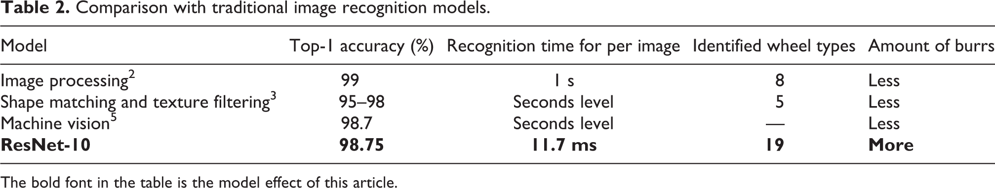
The bold font in the table is the model effect of this article.

Conclusion

The demand for automobile wheel production has been growing rapidly in recent years. This study was aimed at solving a key issue that is often faced in the visual recognition system of automobile wheel production lines. We developed a CNN approach to identify wheel images with complex visual background, which is essential to improve the level of automation required for automobile wheel production lines. In this study, we discussed the development of a CNN-based approach in industrial applications. A traditional image processing method was developed to separate the entire wheel image from the complex background with conveyor belt so that the image was more favorable for deep learning models. By designing the CNN model based on the ResNet, the processed 70,000 wheel images were effectively identified. Our experiment results demonstrated that the recognition rate was achieved over 98% and the single recognition time was 11 ms, both of which met the actual needs of industrial production. Actual implementation of this approach in a wheel production line proved that this method has stronger anti-interference ability than traditional artificial feature recognition methods. As described, traditional image recognition methods based on image processing often require computing hardware and are extremely sensitive to external lighting conditions. Therefore, they cannot solve the problem of identifying wheels with large burrs. To overcome this issue, the CNN program developed here only had a size of only 700 kb to achieve fast implementation. In other words, there is no need for complicated algorithm especially for the millisecond-level recognition speed, which is particularly important for real-world applications.

Footnotes

Declaration of conflicting interests

The author(s) declared no potential conflicts of interest with respect to the research, authorship, and/or publication of this article.

Funding

The author(s) received no financial support for the research, authorship, and/or publication of this article.

ORCID iD

Zheming Tong

References

Zhao

Liu

Automobile wheel recognition system based on machine vision. In: 2007 China Automotive Engineering Society annual meeting, 2007.

Tong

Xin

Tong

, et al. Internal flow structure, fault detection, and performance optimization of centrifugal pumps. J Zhejiang Univ-Sci A 2020;21(2): 85–117.

Cheng

Guan

Zhang

. Automobile wheel hub type identification based on shape matching and texture screening. J Instrum 2017; 38(9): 2299–2306.

Zhu

. The research on recognition and classification technology of aluminum alloy wheel hub. Special Cast Non-Ferr Alloys 2017; 37(6): 619–621.

Guo

Wang

Zhang

. Research on on-line identification and classification technology of wheel based on machine vision. J Test Technol 2019; 33(3): 54–58.

Mourtzis

Vlachou

Milas

. Industrial big data as a result of IoT adoption in manufacturing. Procedia Cirp 2016; 55: 290–295.

Lecun

Bengio

Hinton

. Deep learning. Nature 2015; 521(7553): 436–444.

Krizhevsky

Sutskever

Hinton

. ImageNet classification with deep convolutional neural networks. Adv Neural Inf Process Syst 2012; 25(2).

Cheng

Zhou

. Back cavity character recognition of aluminum wheel based on improved CNN. Comput Eng 2019; 45(05): 188–192.

10.

Hicham

Ahmed

Mohammed

. Vehicle Type Classification Using Convolutional Neural Network. Institute of Electrical and Electronics Engineers Inc, 2018, pp. 313–316.

11.

Keerthi

Gilbert

. Convergence of a generalized SMO algorithm for SVM classifier design. Mach Learn 2002; 46(1–3): 351–360.

12.

Ogata

Yukisawa

Arai

, et al. Automated design of image recognition in capturing environment. IEEJ Trans Electr Electron Eng 2017; 12: S49–S55.

13.

Tong

Huang

Tong

. A robust face recognition method combining LBP with multi-mirror symmetry for images with various face interferences. Int J Autom Comput 2019; 16(5): 671–682.

14.

Tong

Huang

Tong

, et al. A novel short-frequency slip fault energy distribution-based demodulation technique for gear diagnosis and prognosis. Int J Adv Robot Syst 2020; 17(2): 1–16.

15.

Tong

Huang

Jiang

, et al. The identification of gearbox vibration using the meshing impacts based demodulation technique. J Sound Vib 2019; 461: 114879.

16.

Zhou

, et al. Toward new-generation intelligent manufacturing. Engineering 2018; 4(1): 11–20.

17.

. Over-fitting in neural network learning algorithms and its solving strategies. J Vibrat Measure Diagn 2002; 22(4): 260–264.

18.

Prasad

Kumar

Sinha

. Grayscale to color map transformation for efficient image analysis on low processing devices. Adv Intell Syst Comput 2015; 320: 9–18.

19.

Deng

Cahill

. An adaptive Gaussian filter for noise reduction and edge detection. In: 1993 IEEE conference record nuclear science symposium and medical imaging conference, San Francisco, CA, USA, 31 October–6 November 1993, pp. 1615–1619. IEEE.

20.

Zhang

Wang

. Novel survey on the color-image graying algorithm. In: IEEE international conference on computer and information technology, 2017, 7876415, pp. 750–753.

21.

Jones

Shearer

Gates

. Edge extraction algorithm for feather sexing poultry chicks. Trans ASAE 1991; 34(2): 0635–0640.

22.

Mohan

Kanaka Durga

Devathi

, et al. Image processing representation using binary image; grayscale, color image, and histogram. In: Proceedings of the second international conference on computer and communication technologies, 2016, pp. 353–361.

23.

Rajinikanth

Aashiha

Atchaya

. Gray-level histogram based multilevel threshold selection with bat algorithm. Int J Comput Appl 2014; 93: 1–8.

24.

Zhu

Xia

Zhang

, et al. An image segmentation algorithm in image processing based on threshold segmentation. In: International IEEE conference on signal-image technologies and Internet-based system, Shanghai, China, 16–18 December 2007, pp. 673–678. IEEE.

25.

Wang

TY.

The motion detection based on background difference method and active contour model. In: 2011 6th IEEE joint international information technology and artificial intelligence conference, Chongqing, China, 20–22 August 2011, pp. 480–483. IEEE.

26.

Justusson

. Median filtering: Statistical properties. In: Two-Dimensional Digital Signal Prcessing II. Springer Berlin Heidelberg, 1981.

27.

Liu

Wang

Liu

. Preliminary study of using 2D multi-level median filtering technique to eliminate random noises. Oil Geophys Prospect 2005; 40(2): 163–167.

28.

. Median filtering method for image processing and its application. Xidian University of Electronic Technology, 2006.

29.

Canny

. A computational approach to edge detection. IEEE Trans Pattern Anal Mach Intell 1986; PAMI-8(6): 679–698.

30.

Jin

. Improved algorithm for Sobel edge detection of image. J Appl Opt 2008; 29(4): 625–628.

31.

Wang

Liu

. Analysis and research of Sobel operator and Prewitt operator. Comput Digit Eng 2016; 44(10): 2029–2031.

32.

Suzuki

. Topological structural analysis of digitized binary images by border following. Comput Vis Graph Image Process 1985; 30(1): 32–46.

33.

Kaehler

Bradski

. Learning OpenCV 3: computer vision in C++ with the OpenCV Library. O’Reilly Media, Inc. 2016.

34.

Russakovsky

Deng

, et al. ImageNet large scale visual recognition challenge. Int J Comput Vis 2015; 115(3): 211–252.

35.

Simonyan

Zisserman

. Very deep convolutional networks for large-scale image recognition. Comput Sci 2014.

36.

Lin

Chen

Yan

. Network in network. Comput Sci 2013.

37.

Szegedy

Ioffe

Vanhoucke

, et al. Inception-v4, inception-ResNet and the impact of residual connections on learning. AAAI press, 2016. pp. 4278–4284.

38.

Janssen

NAH

van Vliet

PHN

Aarts

, et al. Assessment of exposure to traffic related air pollution of children attending schools near motorways. Atmos Environ 2001; 35(22): 3875–3884.

39.

. On-line learning migration: from social learning theory to social presence theory in a CMC environment. J Netw Comput Appl 2000; 23(1): 27–37.

40.

Klepeis

Nelson

Ott

, et al. The National Human Activity Pattern Survey (NHAPS): a resource for assessing exposure to environmental pollutants. J Expo Sci Environ Epidemiol 2001; 11(3): 231–252.

41.

Abramson

Braverman

Sebestyen

. Pattern recognition and machine learning. IEEE Trans Inform Theory 1963; 9(4): 257–261.

42.

Gnecco

Sanguineti

. The weight-decay technique in learning from data: an optimization point of view. Comput Manage Sci 2009; 6(1): 53–79.

43.

Runnenburg

. Probability theory and its applications. Stat Neerl 2010; 39(2): 181–189.

44.

Uriarte-Arcia

López-Yáñez

Yáñez-Márquez

. One-hot vector hybrid associative classifier for medical data classification. PloS One 2014; 9(4): e95715.

45.

Goldberger

Gordon

Greenspan

An efficient image similarity measure based on approximations of KL-divergence between two Gaussian mixtures. In: Proceedings on ninth IEEE international conference on computer vision, Nice, France, 13–16 October 2003. IEEE.

46.

Horikawa

Furuhashi

Uchikawa

. On fuzzy modeling using fuzzy neural networks with the back-propagation. IEEE Trans Neural Netw 1992; 3(5): 801–806.

47.

Palomar

Jiang

. MIMO transceiver design via majorization theory. A convex optimization theory Foundations and Trends in Communications and Information Theory. 2006; December.

48.

Pun

. A new method for gray-level picture threshold using the entropy of the histogram. Sig Process 1985; 2(3): 223–237.

49.

Chen

Haralick

. Recursive erosion, dilation, opening, and closing transforms. IEEE Trans Image Process 1995; 4(3): 335–345.

50.

Gonzalez

Wintz

. Digital image processing. 4th ed. London: Pearson Education, 2017, p. 1184.

51.

Deng

. Deep learning: methods and applications. Foundat Trend Signal Process 2013; 7(3): 197–387.

A convolutional neural network approach for visual recognition in wheel production lines

Abstract

Keywords

Introduction

Methodology

Image acquisition and preprocessing

Improved image differencing

Edge detection and image segmentation

CNN network model design

Loss function and batch gradient descent algorithm

Result and discussion

Results of image separation in a complex background

Results of visual recognition method

Conclusion

Footnotes

Declaration of conflicting interests

Funding

ORCID iD

References