
Abstract
Using multiple unmanned surface vehicle swarms to implement tasks cooperatively is the most advanced technology in recent years. However, how to find which swarm the unmanned surface vehicle belongs to is a meaningful job. So, this article proposed an artificial potential field-based swarm finding algorithm, which applies the potential field force directly to unmanned surface vehicles and leads them to their belonging swarm quickly and accurately. Meanwhile, the proposed algorithm can also maintain the formation stable while following the desired path. Based on the swarm finding algorithm, the artificial potential field-based collision avoidance method and the International Regulations for Preventing Collisions at Sea-based dynamic collision avoidance strategy are applied to the swarm control of multi-unmanned surface vehicles to enhance the performance in the dynamic ocean environment. Methods in this article are verified through numerical simulations to illustrate the feasibility and effectiveness of proposed schemes.
Introduction
Benefiting from the improvement of the intelligent control, networks and sensors, the unmanned aerial vehicle, the unmanned surface vehicle (USV), and the unmanned underwater vehicle have become the most advanced technologies. Among them, USVs are widely used in both military and civilian. 1 –6 There also have been increasing interests in grouping multi-USVs into a formation to accomplish mission goals cooperatively because of limitations of the single USV operation, such as small mission area and insufficient fault-tolerant resilience.
One of the key issues in the cooperation of multiple USVs is the formation control. Nowadays, there are three dominant approaches being employed to realize the formation control of USVs, including the behavior-based method, 7 –9 the virtual structure approach, 10,11 and the leader–follower method. 12 –16
The fundamental idea of the behavior-based method is to specify various behaviors for all members in the formation and to keep the desired formation by performing prescribed behaviors. This method allows decentralized implementation, but the mathematic model is difficult to build. As for the second approach, all USVs in the formation are seen as a single rigid structure, which is effortless to model but has high requirements of the communication. The third method, namely, the leader–follower method, is used not only in USVs but also in the formation control of mobile robots 17 –19 and autonomous underwater vehicles. 20 –23 The leader sails along a predefined route and followers maintain prescribed distance and orientation with respect to the leader. This method is simple to carry out; however, once the leader is invalid, the entire formation will lose control.
In the three formation control approaches mentioned above, the formation needs to be designed in advance, which limits the flexibility of the formation, and members also lack the autonomy. Whereas the swarm control theory 24 –28 proposed in recent years emphasizes the autonomy and intelligence of members in the formation. Swarm control theory originates from studies of colonies of ants and bees in nature, which has higher flexibility, autonomy, and robustness. Compared with the leader–follower method, a malfunction of one member in the swarm will not cause the loss of the entire formation. So the swarm control theory is more appropriate for the cooperation of multiple USVs in practical applications.
In the formation control of multi-agents, how to find the formation that each agent belongs to and integrate it into its formation are needful jobs. 29 It is also a meaningful issue in the swarm control of multi-USVs, especially the multiple USV swarms (USVSs). The artificial potential field (APF) method is a classic method with a very wide range of applications due to its characteristics of easy modeling, simple mathematic principles, fast response time, and high real-time performance. Moreover, the path calculated by the APF method has good characteristics of smoothness and continuity, which is more suitable for a USV to track. Therefore, in this article, the APF method is used as the core algorithm for the swarm finding of multi-USVs. Meanwhile, the dynamic collision avoidance (DCA) combined with the International Regulations for Preventing Collisions at Sea (COLREGs) are integrated into the swarm control method to enhance the swarm performance in the dynamic ocean environment.
The main contributions of this article are as follows: (1) the APF-based swarm finding algorithm is proposed to lead USVs to their belonging swarms quickly and accurately, it is a needful job especially in the control of multiple USVSs; (2) the path following scheme of the USVS based on the line-of-sight (LOS) guidance law used for the single USV is designed suitable for both straight and curve paths.
The rest of the article is organized as follows: after this “Introduction,” the swarm control strategy composed of the APF-based swarm finding algorithm and the path following scheme are presented in the second section. The COLREGs-based DCA strategy is described in the third section. Numerical simulations are illustrated in the fourth section and conclusions are drawn afterward.
Swarm control strategy
In this article, vectors are bold.
Mathematic model
In this article, USVs are divided into two categories, free-USVs and member-USVs. We consider a USVS is composed of n member-USVs
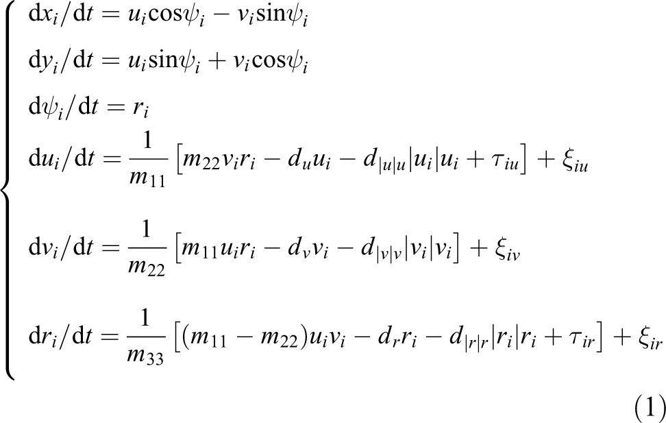
where

where
The illustration and the system configuration of the USVS are shown in Figures 1 and 2. The function of the desired center position of the swarm (CPS) is given by waypoints and the human supervisor in the form as follows

where

Illustration of the USVS. USVS: unmanned surface vehicle swarm.

System configuration of the USVS. USVS: unmanned surface vehicle swarm.
The swarm finding algorithm is utilized according to the function of the desired CPS to attract each free-USV to its swarm. According to the swarm control theory, the intelligence of each USV is emphasized, and the shape of the formation is more flexible. In the work of Tan et al.,
32
the USVS is constructed by the proposed gathering strategy, whereas in this article, an APF-based swarm finding method is utilized to the swarm control of multi-USVs. In the work of Tan et al.,
32
the USVS is built by making the error

where
Here,
Then, the path following scheme and the CA strategy are used to decide the desired speed and heading of each USV. Surge forces and yaw moments of USVs are obtained through the motion planning model and input to the USV dynamics model to calculate their actual positions, velocities, and heading vectors, which are feedback to make the overall system a closed loop.
The swarm control of multi-USVs is mainly based on the APF method to implement the swarm finding and the CA. The total potential field

where
Swarm finding algorithm
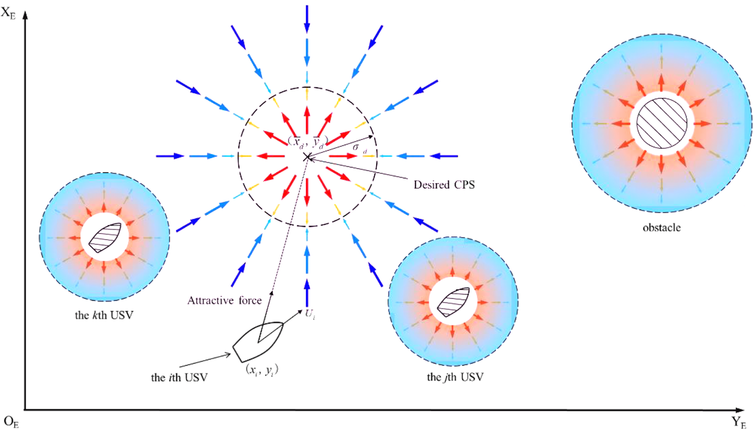
The swarm finding algorithm is used to attract each free-USV to its desired CPS and makes it a member-USV. The illustration of the potential field used in the swarm finding algorithm is presented in Figure 3.

Illustration of the potential field of the swarm finding algorithm.
In this article, each member-USV is required to sail around the desired CPS
The potential field

where

Here,
Given the Euclidean distance between the ith USV and the desired CPS as follows

The potential field function

Taking the gradient of the potential field function

where
Collision avoidance method
Based on the swarm finding algorithm, the APF-based collision avoidance (CA) method is incorporated into the swarm control strategy in this article to accomplish the CA of the inter-USV and the outer-static obstacle.
The schematic of the APF-based CA method used in this article is shown in Figure 4. The fundamental idea in this section is to establish repulsive potential fields
Schematic of the APF-based CA method. APF: artificial potential field; CA: collision avoidance.
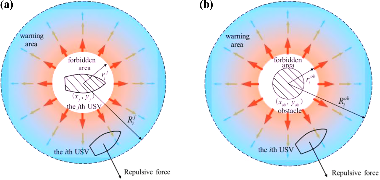
Divisions of the CA area: (a) inter-USV collision avoidance and (b) outer-static obstacle collision avoidance. CA: collision avoidance; USV: unmanned surface vehicle.
Inter-USV CA
The CA between the ith USV and the jth USV is realized by the repulsive potential field

And the repulsive force is given by the gradient of the potential field

where

Outer-static obstacle CA
The APF-based method similar to the CA between USVs is adopted to achieve the CA between the USV and static obstacle. The potential field

where

In equation (16),

where
The potential field function

And the repulsive force is given according to the gradient of the potential field function

where
When the USV enters the warning area of the obstacle and continues to approach it, that is,
Based on the APF-based swarm finding algorithm and CA method described beforehand, the overall potential field

Path following scheme
The fundamental idea of this section is the LOS guidance law, which is used in the path following of the single USV. 33 In the path following scheme of the USVS, the actual CPS, which is regarded as a virtual USV, instead of each single USV in the swarm, is used to track the desired path. Combined with the swarm finding algorithm, each USV can find its swarm and the actual CPS can be calculated using equation (4). The actual CPS tracks the desired path in the light of the LOS guidance law so that the path following of the overall USVS is achieved. The schematic diagram is shown in Figure 6.

Schematic diagram of the USVS path following scheme. USVS: unmanned surface vehicle swarm.
Consider a desired path as

where

where xe
and ye
are the along-following error and the cross-following error, respectively, and
By differentiating equation (22) with respect to time

where

The LOS guidance law of the USVS suitable for both straight and curve paths is designed as follows

where
Based on the designed LOS guidance law, the actual CPS, which is regarded as a virtual USV, can track the desired path so that the path following of the entire USVS is accomplished.
COLREGs-based DCA strategy
Mathematic model
To enhance the safety of the overall USVS in the dynamic ocean environment, the DCA strategy based on the COLREGs 34 is incorporated into the swarm control theory. The illustration of the COLREGs-based DCA strategy is shown in Figure 7.

Illustration of the DCA strategy. DCA: dynamic collision avoidance
Similar to the APF-based CA scheme described before, in the DCA strategy, two areas are also constructed around member-USVs in swarm, namely, the forbidden area and the warning area. However, to achieve the DCA, position vectors and orientations rather than the APF method are used to keep the closest point of approach (DCPA) greater than a threshold value when the USV encounters a moving obstacle ship. The minimum threshold value of the DCPA is defined as DCPAs. If the DCPA less than the DCPAs, it can be considered the USV is in a risk of collision, and the DCA strategy should be adopted to eliminate the collision danger.
As shown in Figure 7, the ith USV with the speed of Ui
and the heading angle

where


The relative velocity of these two vessels is given as

And the angle of the relative velocity is

The value of

And the value of
There may be a high probability the USV could encounter moving obstacle ships continuously in the complex marine environment. So, to decide which obstacle ship the USV should avoid first, the DCA priority

where
Conclusion could be given as the smaller
DCA maneuvers
Based on the priority
DCA maneuvers proposed in this article are designed mainly according to the rules 13–17 of COLREGs, which are given in five cases as follows: Head-on Crossing from right Crossing from left Overtaking Being overtaken
Numerical simulations
Two computer-based numerical simulations have been implemented using MATLAB (R2016b) to verify the performance of the proposed algorithms. The first simulation focused on testing the effect of the APF-based swarm finding algorithm combined with the CA method and the path following scheme of two USVSs in the static environment. Then, all these algorithms are applied to a USVS united with the COLREGs-based DCA strategy in a realistic environment of two moving obstacle ships in the second simulation to validate the feasibility of the overall USVS in the dynamic environment. Dimensions and movement parameters of the USVs 28 used in these two simulations are shown in Table 1, and general parameters of simulations are listed in Table 2.
Dimensions and movement parameters.
General parameters of the simulations.

Simulation in the static environment
In the process of performing tasks via multiple USVSs corporately, how to find the swarm that the USV belongs to quickly and accurately is a meaningful job, especially in the case when the USV sails from one swarm to another during the execution of tasks. So, for the purpose of verifying the performance of the APF-based swarm finding algorithm in the situation mentioned above, eight USVs are divided into two swarms to perform different missions sailing along two perpendicular desired paths separately, and during this process, four USVs change their tasks and enter each other’s swarm at the intersection of paths. Two static obstacles are set in this process to test the effect of the CA method.
Sailing trajectories of eight USVs are presented in Figure 8, and six detailed plots of specific locations on the trajectories are given in Figure 9.

Sailing trajectories in the static environment. USV: unmanned surface vehicle; CPS: center position of the swarm.

Detailed plots: (a) t = 0 s, (b) t = 120–220 s, (c) t = 120–220 s, (d) t = 240–350 s, (e) t = 400–450 s, and (f) t = 400–450 s. USV: unmanned surface vehicle; CPS: center position of the swarm.
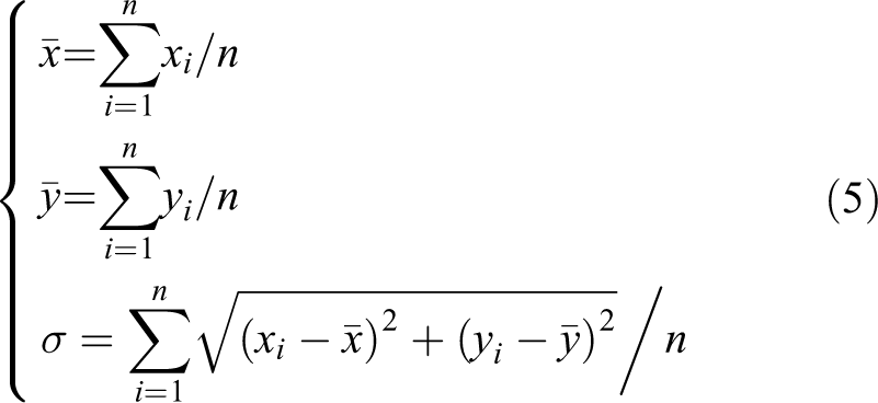
To perform different tasks, eight USVs are divided into two groups sailing from the initial positions at (150,300), (150,350), (150,400), (150,450), (100,300), (100,350), (100,400), (100,450), respectively. As shown in Figure 9(a), actual CPSs of these two groups locate at (125,425), (125,325), and average DVs are about 36.36 m.
Under the effect of the proposed swarm finding algorithm, two groups of free-USVs are attracted to their desired CPS given by the waypoints of the desired paths, which are (150,1000), (550,1000), (950,1000), (1350,1000) of swarm1 and (750,400), (750,800), (750,1200), (750,1600) of swarm2, separately. Stable formations of two USVSs are formed quickly at the initial stage and the actual CPS, which is viewed as a virtual leader, is utilized to guide the path following of the USVS according to the LOS guidance law. As shown in Figure 8, formations of member-USVs are always maintained while sailing along the desired path, except for some slight deformations near the obstacles.
In this simulation, two static obstacles are set on the way of desired paths to test the performance of the CA method and two detailed views are represented in Figure 9(b) and (c). It can be seen from figures that actual CPSs of two swarms lie on the desired paths and member-USVs in swarm sail around the actual CPS so that the path following of each USVS is achieved. When the USV approaches the obstacle, it is repelled by the potential field so that the sailing trajectory keeps safe distance to the obstacle. After passing by the obstacle, average DVs of two swarms increase from 36.36 m to about 46 m. So there are slight deformations in the process of the CA. However, the formation is stabilized gradually afterward. So, USVs in the swarm have good security and high performance of the CA.
After the avoidance of static obstacles, two swarms continue to sail until they reach the intersection of two desired paths. At this moment, USV3, USV4 in the group1 and USV1, USV2 in the group2 exchange the tasks they perform so that these four USVs change their formations and enter each other’s swarm as shown in Figure 9(d). Afterward, two swarms, which are swarm1 composed of USV1, USV2 in the group1 united with USV1, USV2 from the group2 and swarm2 composed of USV3, USV4 in the group2 united with USV3, USV4 from the group1, continue to carry out their missions sailing along the desired paths. USVs that change their missions can find the swarm they belong to accurately and new swarms are formed quickly under the effect of the swarm finding algorithm. Because of the effect of the inter-USV CA method, there are no collision risks in the process of integrating new USVs into the swarm.
As shown in Figure 9(e) and (f), new USVSs continue to sail along the desired paths until arriving at the target points after exchanging their tasks. And average DVs of two swarms are about 33 and 34 m.
Time history curves of course and speed of the USV2 in group2 are shown in Figure 10(a) and (b). Curves remain stable at most of the time but vary greatly in the time span of 150–220 s and 260–340 s, in which the USV2 avoids the static obstacle and is guided from the swarm2 to the swarm1 under the effect of the swarm finding algorithm, separately.
(a) Course and (b) speed of USV2 in group2. USV: unmanned surface vehicle.
Time history curves of distances between USV2 in group2 and other USVs are shown in Figure 11. In the first 150 s, distances between USV2 and USV1, USV3, USV4 in group2 remain stable, which means that these four USVs maintain a stable formation so that the swarm2 is constructed in this process. Then at about 200 s, distances between USV2 and USV3, USV4 increase but distance between USV2 and USV1 decreases, which is due to the CA of the static obstacle in the time span of 150–220 s. Afterward, at about 300 s, distances between USV2 and USV3, USV4 in group2 start to increase significantly, whereas distances between USV2 in group2 and USV1, USV2 in group1 keep a low level until they reach the target point. It means that in the last 150 s, USV1, USV2 in group2 and USV1, USV2 in group1 form a new stable swarm and sail along the desired path together toward the target.

Distances between USV2 in group2 and other USVs. USV: unmanned surface vehicle.
From all results of the first simulation presented before, it can be concluded that the USV can find its swarm accurately and the formation can be constructed quickly under the effect of the proposed swarm finding algorithm. The CA between inter-USVs and static obstacles in this process is accomplished, and the straight line path following of the USVS is also realized. The overall USVS is stable and has a good performance of security in the static environment.
Simulation in the dynamic environment
The feasibility of the overall USVS in the dynamic environment is validated in this section. All algorithms aforementioned united with the COLREGs-based DCA strategy are applied to a swarm of four USVs sailing along a desired path in an environment of two moving obstacle ships. Under the effect of the swarm finding algorithm, four USVs are attracted to their belonging swarm from the start point and sail along the desired path toward the target; in this process, two moving obstacle ships and three static obstacles are set to verify the safety of the USVS.
Sailing trajectories of four USVs are given in Figure 12, and three detailed plots are shown in Figure 13.

Sailing trajectories in the dynamic environment. USV: unmanned surface vehicle; CPS: center position of the swarm.

Detailed plots: (a) t = 40–90 s, (b) t = 350–420 s, and (c) t = 150–280 s. USV: unmanned surface vehicle; CPS: center position of the swarm.
Four free-USVs start from points (50,0), (0,100), (100,50), (50,250) and are attracted to their desired CPS under the effect of the swarm finding algorithm. It is clearly seen that changes in the sailing trajectories of four USVs in the swarm finding process. Then, these four USVs have stable positions in the formation, so they become the member-USVs and the swarm is constructed.
As shown in Figure 13(a), the USVS tracks the desired path until meeting the first moving obstacle ship, which sails from the right side of the swarm. As described in the “DCA maneuvers” section, all USVs are in the state of “give-way” and are required to turn to their starboards to avoid the obstacle ship. As can be seen in the figure, USV1, USV2, and USV4 perform the DCA behaviors but USV3 does not. It is because that when the USVS encounters the first moving obstacle ship, the obstacle ship does not lie inside the warning area of the USV3, so it can be considered that there is no danger of collision for the USV3. After avoiding the first obstacle ship, the actual CPS locates near the desired path and the average DV of the USVS is about 38 m.
Then, the USVS passes a desired curve path and sails through three static obstacles, as shown in Figure 13(c). All USVs in the swarm avoid obstacles successfully and their sailing trajectories keep safe distances to obstacles. There is a deviation in the path following because of avoiding static obstacles, and the average DV is about 42 m. Same as the situation in the first simulation,
Afterward, the USVS passes a desired curve path again and continues to sail until meeting the second moving obstacle ship which sails toward the swarm, as shown in Figure 13(b). In this article, for the purpose of simplifying the simulation, movements of all obstacle ships will not change. So, it can be seen that USV1 and USV2 turn to their starboards to avoid the obstacle ship on its port side, however, USV3 and USV4, which are in no collision risks, do not employ DCA behaviors. The average DV in this process is about 31 m.
Time curves of course and speed of the USV2 in swarm are shown in Figure 14(a) and (b). There is a saltation in the course at about 225 s when the USV2 avoids the third static obstacle and the course exceeds

(a) Course and (b) speed of USV2 in swarm. USV: unmanned surface vehicle.
Errors of the USVS path following in the dynamic environment, namely, the along-following error, the cross-following error, and the error between

Errors of the USVS path following. USVS: unmanned surface vehicle swarm.
Conclusions
This article presents an APF-based swarm finding approach for multi-USVs in both static and dynamic environment. LOS-based path following scheme and COLREGs-based DCA maneuvers are integrated to enhance the performance of the USVS. All algorithms proposed in this article are verified by numerical simulations. From the results of two simulations, the free-USVs can find their belonging swarm quickly under the proposed swarm finding algorithm and can form a stable formation sailing along the desired path. Combined with multiple CA methods defined in this article, the USVS has a good performance of security and can strictly adhere to the COLREGs in the dynamic marine environment.
However, in this article, only moving obstacle ships of regular movements are considered for the sake of simplifying the simulation. Therefore, in our future research, the prediction and acquisition of the movement of obstacle ships via neural networks will be focused on.
Footnotes
Declaration of conflicting interests
The author(s) declared no potential conflicts of interest with respect to the research, authorship, and/or publication of this article.
Funding
The author(s) disclosed receipt of the following financial support for the research, authorship, and/or publication of this article: This work was supported by the Opening Foundation of State Key Laboratory of Ocean Engineering (no. 1617), the Laboratory Foundation of Science and Technology on Water Jet Propulsion (no. 614222303030917), Foundation Research Funds for the Central Universities (no. HEUCFJ170110 and no. HEUCFM170101) and the National Natural Science Foundation of China (nos 51409054 and 51509055).