Sage Journals: Discover world-class research

Abstract

The aim of this article is to present a statistical comparison of the electric energy expenditure between two techniques for the generation of gait patterns in biped robots. The first one is to minimize the sum of the squared torques applied to the joints of the robot, and the second one is based on the cart-table model. For the experiments, we measured the energy delivered by the battery of the robot to the servomotors. We applied the two aforementioned methods for three velocities (0.5, 1.0, and 1.3 m/min). Additionally, each combination of method and velocity was performed by the robot 10 times. The energy expenditure for each method was compared by applying the Wilcoxon test. In all comparisons, the value of p was lower than 0.004, indicating that the differences were statistically significant. The optimization approach leads to a reduction in energy expenditure that ranged from 9.16 % to 13.35 %. The conclusion is that all the effort required to implement an approach that requires a complete dynamic model of the robot allows a significant reduction in energy consumption.

Keywords

Biped robot energy consumption trajectories generation optimization

Introduction

Robots and mechatronic systems are required to be energetically efficient, especially when they are conceived for high-speed continuous operations.¹ In the case of robotic manipulators, this topic has received considerable attention of many researchers, and as a consequence, different optimization solutions have been proposed. Woolfrey et al.² proposed a torque minimization approach to resolve redundancy in manipulators that handle large external forces. In the study of Trigatti et al.,³ a trajectory planning strategy for spray painting robots is presented.

The problem of efficiency has also been addressed in biped robots because their autonomous operation requires independent energy sources such as batteries. These solutions can be oriented to modify the mechanical structure of the robot, for example, introducing torsion springs between the joints and the actuators.^1,4,5 However, as stated by Scalera et al.,¹ the main drawback of these solutions is that the stiffness of the springs cannot be adapted to different motions. Other approaches are oriented to modify the motion patterns of the robot. Currently, there are two main approaches to the generation of biped robot trajectories. One of them is known as the cart-table approach, which involves only the kinematic model of the biped and its total mass.^6

–9 The mass of the car symbolizes the total mass of the robot, and its location corresponds to the center of mass (CoM) of the biped.^10,11 This method is used by bipeds such as ASIMO,^12,13 HRP,^14
–16 Nao,^17,18 HUBO,¹⁹ and ATLAS.^20,21 The other approach is based on numerical optimization. It considers all the components of a Lagrangian model, such as the inertia matrix, and the vectors of centrifugal, gravitational, Coriolis, and friction forces. An example of this approach is the technique proposed by Chevallereau and Aoustin²² based on the minimization of the average energy expended by the robot. In this approach, two cost functions are considered. One of them is the time-integral of the squared Euclidean norm of the torques applied to robot joints. This variable is a surrogate of Joule effect losses^23,24 when the relationship between the current delivered to electric motors and the joint torques is linear. The second cost function is the time-integral of the absolute value of the dot product between the torques and the angular velocities.^25,26 The main limitation of the aforementioned optimization schemes is that the convergence to a global minimum cannot be guaranteed.²⁷ Furthermore, even in the case that this convergence could be guaranteed, the differences between the dynamic of the real robot and that of the model used by the optimization algorithm convert the resulting trajectories into suboptimal. One of the sources for these differences are model actuators.^22,28,29 For example, when magnetic saturation exists in an electrical motor, the nonlinear equation that relates flux and armature current is difficult to obtain and, as a consequence, is not considered in the dynamic model.^30,31 Another factor that hinders the adoption of the numerical optimization approaches is their high computational cost. In the case of the current article, for example, the minimization space is composed of 60 dimensions.

Despite all the difficulties presented in the previous paragraph, optimization approaches based on Lagrangian models have been applied to biped robots. The largest part of these works present simulation results,^27,32
–34 whereas the number of experimental studies is still scarce.^25,35 This imbalance is due to the fact that most simulation studies use simplified models, which are very valuable as proof of concept, but which cannot be considered valid mathematical representations of real robots. For example, in the study of Roussel et al.,³² the Coriolis matrix is not considered, and the studies by Huang and Hase³³ and Tlalolini et al.³⁴ consider bidimensional prototypes. Unlike the previous ones, the study of Tlalolini et al.²⁷ presents a three-dimensional model with 14 joints. Another factor reducing the number of experimental evaluations of energy consumption is the need to modify the biped to add a current and voltage monitoring system.

In this article, two techniques for the generation of gait patterns in biped robots are compared. The first one is to minimize the sum of the squared torques applied to the joints of the robot, and the second one is based on the cart-table model. The aim of this work is to contribute with experimental evidence to answer the following question: Does the generation of trajectories based on numerical optimization lead to significant energy savings compared to the cart-table method? In addition, a penalty-based optimization approach that allows to generate joint trajectories of minimal energy expenditure in biped robots is proposed. Another contribution of the present work is a sound statistical framework to compare the energy expenditure of gait trajectories in biped robots.

Bioloid robot

The Bioloid humanoid (type A) from Robotis is an 18-degree-of-freedom (DOF) robot, with 6 DOFs in each leg (see Figure 1). Each actuator is an AX-12A servo with position measurement of 0.29° resolution. These servos are controlled by the CM-530 board. When the stabilizing functionality is activated, a gyro sensor provides the angular rates around the anterior–posterior and medial–lateral axis to the CM-530, which modifies the trajectories of the servos. In Bioloid robots, the torques applied to the joints are not defined by the user but by proportional derivative (PD) controllers implemented as closed source firmware.

Figure 1.

Bioloid humanoid robot (type A).

CAD model

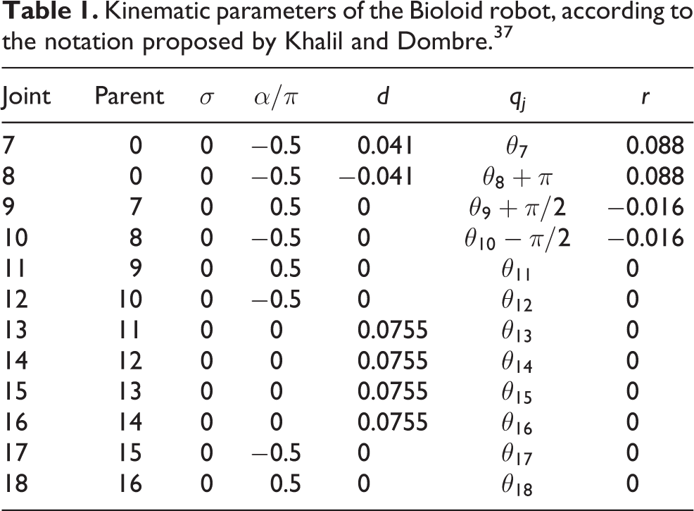
The inertia moments and the CoMs of the robot were obtained from the computer-aided design (CAD) models provided by Robotis. Currently, it is unknown if these parameters include the contributions from electronics boards, wiring, and hollow spaces in plastic body. However, even if the CAD model is perfect, there are real-world phenomena that our model do not take into account or cannot be identified, as mechanical backlash in the gears, as well as the dead band of the PD controllers. The dynamical model of the robot was found using the Newton–Euler algorithm.^36,37

Dynamic model of the robot

The Lagrangian representation of the robot is as follows

A (q) q_{a} + H (q, q_{v}) = B Γ + J_{r}^{T} (q) F_{r} + J_{l}^{T} (q) F_{l}

where $q \in I R^{18}$ is the vector of generalized coordinates. This vector contains (i) $(^{0} x_{g},^{0} y_{g},^{0} z_{g})$ that are the Cartesian position of the trunk frame $< x_{0}, y_{0}, z_{0} >$ with respect to the ground frame $< x_{g}, y_{g}, z_{g} >$ (see Figure 2), (ii) $σ = {ϕ, θ, ψ}$ are the Euler angles describing the orientation of the trunk frame $< x_{0}, y_{0}, z_{0} >$ with respect to the ground frame $< x_{g}, y_{g}, z_{g} >$ , and (iii) $(q_{7}, \dots, q_{18})$ are the 12 joint positions of the legs

\begin{array}{l} q & = {[\begin{matrix} ^{g} x_{0} & ^{g} y_{0} & ^{g} z_{0} & ϕ & θ & ψ & \dots & q_{7} & \dots & q_{18} \end{matrix}]}^{T} \\ q_{v} & = {[\begin{matrix} ^{g} {\dot{x}}_{0} & ^{g} {\dot{y}}_{0} & ^{g} {\dot{z}}_{0} & ^{0} ω_{0x} & ^{0} ω_{0y} & ^{0} ω_{0z} & {\dot{q}}_{7} & \dots & {\dot{q}}_{18} \end{matrix}]}^{T} \\ q_{a} & = {[\begin{matrix} ^{g} {\ddot{x}}_{0} & ^{g} {\ddot{y}}_{0} & ^{g} {\ddot{z}}_{0} & ^{0} {\dot{ω}}_{0x} & ^{0} {\dot{ω}}_{0y} & ^{0} {\dot{ω}}_{0z} & {\ddot{q}}_{7} & \dots & {\ddot{q}}_{18} \end{matrix}]}^{T} \end{array}

Figure 2.

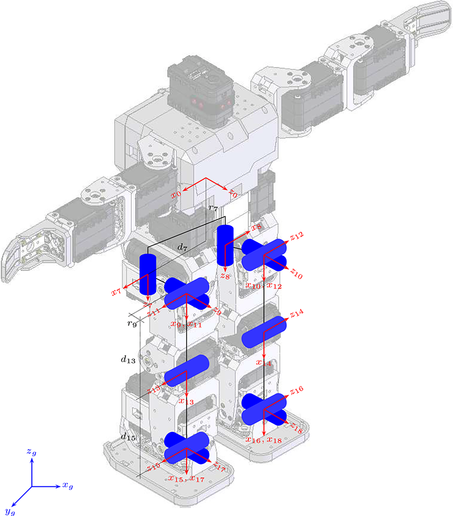
Reference frames and joint angles convention.

$q_{v} \in I R^{18}$ is the vector of generalized velocities and $q_{a} \in I R^{18}$ is the vector of generalized accelerations. $A \in I R^{18 \times 18}$ is the inertia matrix. $H \in I R^{18}$ is the vector of centrifugal, gravitational, and Coriolis forces. $B \in I R^{18 \times 12}$ is the actuation matrix that contains only ones and zeros. The first six rows of $B$ are zero, indicating that $Γ$ has no direct influence on components 1–6 of q_a . The following $12$ rows of $B$ form an identity matrix, indicating that $Γ_{i} (i = 7, \dots,18)$ directly affects the component i of the vector q_a . The vector $Γ \in I R^{12}$ contains the torques applied to the joints of the robot. This leads $B$ to satisfy the following property

B Γ = [\begin{matrix} 0_{6 \times 12} \\ Γ \end{matrix}]

$J_{r} ≜ {}^{g}J_{17} \in I R^{6 \times 18}$ is the Jacobian matrix relating the linear and angular velocities of the robot’s right foot with the vector q_v . The super index g indicates that a variable is expressed in the ground frame

[\begin{matrix} ^{g} v_{17} \\ ^{g} ω_{17} \end{matrix}] = {}^{g}J_{17} (q) \cdot q_{v}

In equation (4), $^{g} v_{17}$ and $^{g} ω_{17}$ are the linear and the angular velocities of the frame $< x_{17}, y_{17}, z_{17} >$ with respect to $< x_{g}, y_{g}, z_{g} >$ . $J_{l} ≜ {}^{g}J_{18} \in I R^{6 \times 18}$ is the Jacobian matrix relating the linear and angular velocities of the robot’s left foot with the vector q_v

[\begin{matrix} ^{g} v_{18} \\ ^{g} ω_{18} \end{matrix}] = {}^{g}J_{18} (q) \cdot q_{v}

In equation (5), $^{g} v_{18}$ and $^{g} ω_{18}$ are the linear and angular velocities of the frame $< x_{18}, y_{18}, z_{18} >$ with respect to $< x_{g}, y_{g}, z_{g} >$ . The $F_{r} \in I R^{6}$ and $F_{l} \in I R^{6}$ contain the resulting of the contact forces between feet and ground. The six elements of the vector F_r are the normal force $f_{n_{r}} \in I R$ , the tangential reaction forces $f_{t_{r}} \in I R^{2}$ , and the ground reaction torques $Γ_{c_{r}} \in I R^{3}$ . The components of F_l are defined similarly to those of F_r . When the left foot is in swing phase, then $F_{l} = 0$ , and the unknowns of the model 1 are $q_{a} \in I R^{18}$ and $F_{r} \in I R^{6}$ . In such a case, there are $12$ equations and $18$ variables. The additional equations are obtained by taking into consideration that right foot does not move with respect to the ground reference frame. This constraint implies that the time-derivative of the right hand side of equation (4) is zero. Thus, when $F_{l} = 0$ , the dynamical model is as follows

[\begin{matrix} A (q) & - J_{r}^{T} (q) \\ J_{r} (q) & 0 \end{matrix}] [\begin{matrix} q_{a} \\ F_{r} \end{matrix}] = [\begin{matrix} B Γ - H (q, q_{v}) \\ - {\dot{J}}_{r} (q) q_{v} \end{matrix}]

The term ${\dot{J}}_{r} (q) q_{v}$ is calculated by using the Newton–Euler algorithm.^36,37 The above described procedure can be applied to the other phases of gait. The kinematic and the dynamic parameters of the model equation (1) are presented in Tables 1 and 2, respectively.

Table 1.

Kinematic parameters of the Bioloid robot, according to the notation proposed by Khalil and Dombre.³⁷

Joint	Parent	$α / π$	d	q_j	r
7	0	−0.5	0.041	$θ_{7}$	0.088
8	0	−0.5	−0.041	$θ_{8} + π$	0.088
9	7	0.5	0	$θ_{9} + π / 2$	−0.016
10	8	−0.5	0	$θ_{10} - π / 2$	−0.016
11	9	0.5	0	$θ_{11}$	0
12	10	−0.5	0	$θ_{12}$	0
13	11	0	0.0755	$θ_{13}$	0
14	12	0	0.0755	$θ_{14}$	0
15	13	0	0.0755	$θ_{15}$	0
16	14	0	0.0755	$θ_{16}$	0
17	15	−0.5	0	$θ_{17}$	0
18	16	0.5	0	$θ_{18}$	0

Table 2.

Dynamic parameters of the Bioloid robot.^a

Joint	$I_{x x}$	$I_{x y}$	$I_{x z}$	$I_{y y}$	$I_{y z}$	$I_{x x}$	m_x	m_y	m_z	M
0	0.00113	−6.01e−06	−1.62e−05	0.00105	0.0002	0.00109	0.000695	−0.00417	0.0132	0.7
7	7.4e−06	0	5.5e−10	4.43e−06	0	4.26e−06	0	0	−0.000166	0.0108
8	7.4e−06	0	−5.5e−10	4.43e−06	0	4.26e−06	0	0	−0.000166	0.0108
9	1.13e−05	4.37e−06	−9.18e−07	9.65e−05	1.23e−07	9.54e−05	−6.3e−05	0.00218	−0.00521	0.137
10	0.00026	−1.07e−06	−8.13e−05	0.00029	1.45e−06	4.21e−05	0.00206	−0.00219	0.00219	0.137
11	1.39e−05	−3.07e−06	0	8.68e−05	0	7.84e−05	0.00138	−3.77e−05	0	0.0312
12	1.39e−05	3.07e−06	0	8.68e−05	0	7.84e−05	0.00138	3.77e−05	0	0.0312
13	1.37e−05	−1.09e−06	1.92e−06	5.43e−05	−2.12e−07	4.79e−05	0.000627	−8.74e−05	0.00011	0.0865
14	1.36e−05	1.09e−06	9.59e−07	5.42e−05	1.25e−07	4.79e−05	0.000627	8.74e−05	0.00011	0.0865
15	0.000279	8.48e−05	1.07e−06	4.21e−05	1.55e−06	0.00309	−0.00206	−0.00219	−6.3e−05	0.137
16	8.91e−05	−5.92e−05	1.98e−06	0.000108	−1.09e−07	0.000184	−0.00206	0.00219	−6.3e−05	0.137
17	4.12e−05	−5.16e−06	5.31e−06	5.91e−05	−1.42e−06	3.7e−05	0.000958	−0.00017	0.00017	0.0374
18	4.11e−05	5.09e−06	5.31e−06	5.91e−05	1.39e−06	3.69e−05	0.000958	0.000168	0.000175	0.0374

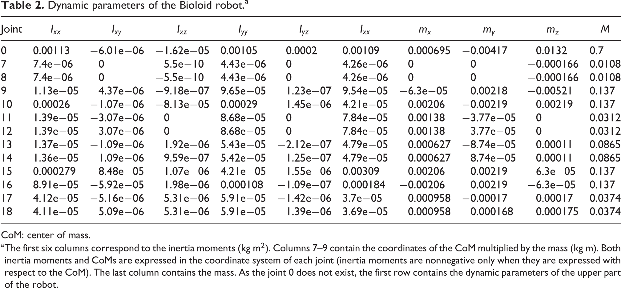
CoM: center of mass.

^a The first six columns correspond to the inertia moments ( $kg m^{2}$ ). Columns 7–9 contain the coordinates of the CoM multiplied by the mass ( $kg m$ ). Both inertia moments and CoMs are expressed in the coordinate system of each joint (inertia moments are nonnegative only when they are expressed with respect to the CoM). The last column contains the mass. As the joint 0 does not exist, the first row contains the dynamic parameters of the upper part of the robot.

Materials and methods

Energy expenditure measurement system

The energy consumption measurement system developed by authors (see Figure 3) is composed of four electronic modules and a software component. The electronic subsystems are:

The DC power supply module: It utilizes a 12 V and 2200 mAH lithium-polymer (LIPO) battery to feed the motors and all electronic components, including those added to measure energy consumption. The power supply module includes external regulators to ensure that the reference for the analog to digital converters (ADC) of the Arduino Nano V3 board remains constant despite the voltage fluctuations across the terminals of the LIPO battery. This aspect is of capital importance to guarantee the reliability of the measurements delivered by the ADCs.

The current measurement module: It measures the current delivered by the LIPO battery. This is done by using a shunt resistance of $0.28 Ω$ ( $1 %$ of tolerance, $4 W$ ) and a differential amplifier, following the scheme proposed in the study of Regan et al.³⁸ The output of the differential amplifier is connected to one of the ADCs of the Arduino Nano V3 board.

The voltage measurement module: It measures the voltage between the terminals of the LIPO battery. As the battery voltage is 12 V and the input to the ADCs of the Arduino Nano must range from 0 to 5 V, a voltage divider of gain $2 / 5$ followed by a unit gain amplifier were used.

The wireless transmission module: It uses a Bluetooth HC-05 board to send every 50 ms the voltage and the current measured by the Arduino Nano board to a computer running Matlab R2018b (The MathWorks, Inc., Natick, Massachusetts, USA).

Figure 3.

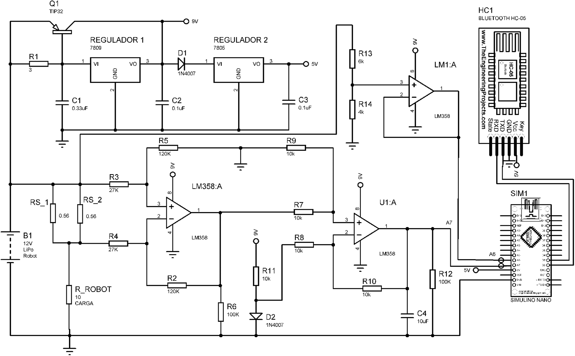
Electronic board for calculating power and energy consumption.

The weight of the board containing the energy measurement system is 100 g, and its dimensions are 7 × 10 cm². The software component stores the voltage and current samples sent by the wireless transmission module and calculates power and energy consumption. This last variable is calculated by using the trapezoidal integration.

Joint trajectory convention

For trajectory generation, we considered the 12 joints belonging to the legs (see Figure 2). The six joints for the right leg are $q_{7}, q_{9}, q_{11}, q_{13}, q_{15}$ , and $q_{17}$ , and the joints for the left leg are $q_{8}, q_{10}, q_{12}, q_{14}, q_{16}$ , and $q_{18}$ . Each hip has three DOFs. The joints q ₇ and q ₈ allow hip rotation in the transverse plane, q ₉ and $q_{10}$ in the frontal plane, and $q_{11}$ and $q_{12}$ in the sagittal plane. The knee has one DOF in the sagittal plane, $q_{13}$ for the right leg and $q_{14}$ for the left leg. The ankle has two DOFs. The joints $q_{15}$ and $q_{16}$ allow ankle rotation in the sagittal plane and $q_{17}$ and $q_{18}$ in the frontal plane.

Trajectory generation using the cart-table approach

The cart-table approach, described in the literature,^10,11 is based on the following assumptions: (i) Robot walks on flat surface perpendicular to the gravity axis. (ii) The spatial trajectories of both feet are the same. (iii) There is a double support phase. (iv) The height of the CoM with respect to the ground is assumed constant. (v) In the contact stage, the foot reaches parallel to the ground. Under the above assumptions, the relationship between the Cartesian position of the zero moment point³⁹ (ZMP) and the projection on the ground of the CoM is described by equation (7)

\begin{array}{l} P_{{ZMP}_{x}} & = x - \frac{z_{c}}{g} \ddot{x} \\ P_{{ZMP}_{y}} & = y - \frac{z_{c}}{g} \ddot{y} \end{array}

where g is the Earth’s gravity. The constant z_c is the desired height of the CoM. The pair $(P_{{ZMP}_{x}}, P_{{ZMP}_{y}})$ is the Cartesian position of the ZMP and $(x, y)$ is the Cartesian position of the CoM. The axis x is parallel to the gait direction and y is perpendicular to it. The eigenvalues of the linear differential equation (7) are $+ \sqrt{g / Z_{c}}$ and $- \sqrt{g / Z_{c}}$ , and consequently the dynamics is unstable. That means that given the input $P_{{ZMP}_{x}} (t)$ and $P_{{ZMP}_{y}} (t)$ , the resulting solutions $x (t)$ and $y (t)$ will tend to infinity. An approximate but bounded-output solution of equation (7) can be obtained by applying the preview control method described by Kajita et al.¹⁰ The following is the procedure to obtain the joint angles:

Select the trajectory of each foot. This requires defining both the parameters presented in Table 3 and the dimensions of the each foot (10 × 6 cm²). The trajectories of the feet are the inverted parabolas presented in Figure 4.

Define the ZMP trajectory $(P_{{ZMP}_{x}}, P_{{ZMP}_{y}})$ . This is done by fixing a set of intermediate points and then interpolating. Most works use linear interpolation, and therefore the ZMP trajectory has a triangular shape.^10,41,42 In the current case, we use cubic splines to interpolate the midpoints presented in Table 4.

Calculate the trajectory of the COM by applying the preview control and using the ZMP obtained in the previous step as the reference signal.

Obtain the joint angles by using the trajectories of the COM and the feet as inputs to the inverse kinematic model.

Table 3.

Parameters for cart-table joint trajectory generation.

Parameter	Description	Value
z_c	Desired height of CoM	$21.3 \times 10^{- 2} m$
L_p	Step length	$4 \times 10^{- 2} m$
W_p	Step width	$8 \times 10^{- 2} m$
A_p	Maximal foot height during swing phase	$4 \times 10^{- 2} m$
T	Step duration	$2 s$
$T_{d s}$	Double support time $(T_{d s} = 0.2 T_{p})$ ⁴⁰	$0.4 s$
h	Sampling time	$0.005 s$

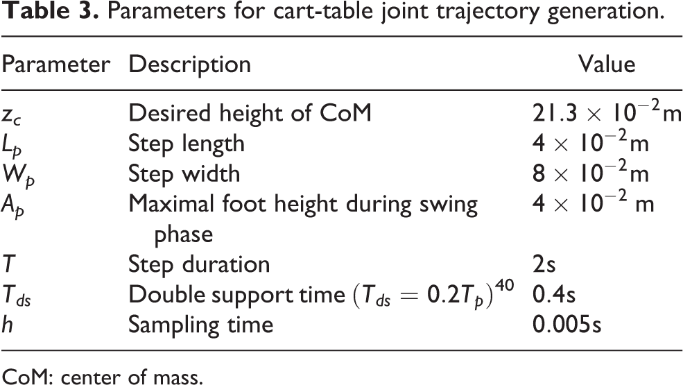
CoM: center of mass.

Figure 4.

Cartesian feet trajectory. Red line corresponds to right foot trajectory and blue line to left foot trajectory. The rectangle black line represents the foot surface.

Table 4.

Intermediate points for the ZMP.

Time	$P_{{ZMP}_{x}}$	$P_{{ZMP}_{y}}$
0.0	0.00	0.04
0.3	0.00	0.00
1.2	0.02	0.08
2.1	0.04	0.00
3.0	0.06	0.08
3.9	0.08	0.00
4.8	0.10	0.08
5.7	0.12	0.00
6.0	0.12	0.04

ZMP: zero moment point.

Trajectory generation using the optimization approach

The purpose of the optimization approaches for the generation of gait patterns in bipedal robots is to find the articular trajectories that minimize a performance index, such as the torques exerted by the actuators or the mechanical energy expenditure. The criterion used in this work was proposed by Chevallereau and Aoustin²² and Saidouni.²³ It consists of minimizing the functional described by equation (8), which is related to the energy losses in the actuators of the robot

J = \int_{0}^{T} Γ^{T} (q, q_{v}, q_{a}) Γ (q, q_{v}, q_{a}) d t

The vector $Γ (q, q_{v}, q_{a})$ represents the torques exerted by the actuators as a function of generalized positions q, velocities q_v , and accelerations q_a . The numerical value of $Γ (q, q_{v}, q_{a})$ is calculated by using the inverse dynamic model of the robot. To transform the variational calculus problem defined by equation (8) into a parametric optimization problem, the angular positions must be defined in terms of a finite set of parameters. In this way, minimizing J no longer requires finding a function of time $q (t)$ , but a vector of parameters, which is easier to find numerically. The only difference between our approach and the one proposed by Chevallereau and Aoustin²² is the parametrization of $q (t)$ . In that study,²² the authors use fourth-order polynomials, and in our case a truncated Fourier expansion, which we consider more appropriate for periodic signals. In the present work, the angular trajectory of the joint i is parametrized in terms of the $2 N + 1$ coefficients defined by equation (9)

q_{i} (t) = \frac{a_{i,0}}{2} + \sum_{n = 1}^{N} a_{i, n} cos (n ω_{0} t) + b_{i, n} sin (n ω_{0} t)

$ω_{0} = 2 π / T$ is the fundamental frequency of $q_{i} (t)$ . The variable T represents the duration of the step (see Table 3). As a part of this study, the value of N was changed from 1 to 5 to see its effect in the performance index J (see equation (8)). A set of coefficients for equation (9) is considered feasible if the resulting trajectories satisfy the following equality and inequality conditions for $0 \leq t \leq T$ .²²

Inequality constraints:

I ₁: When there is contact between one foot and the ground, the resulting normal reaction forces must be positive. That means that reaction forces can prevent interpenetration between the foot and the ground but cannot stick the foot to the ground

f_{n_{r}} \geq 0

I ₂: When there is contact between one foot and the ground, the resulting tangential reaction forces must be in the friction cone to avoid slipping (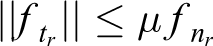 $μ$ is the Coulomb friction)

| | f_{t_{r}} | | \leq μ f_{n_{r}}

I ₃: The absolute value of the joint torques must be less than $15 kg \cdot cm$ , which is the maximum torque that the Dynamixel AX12 servos can exert

| Γ_{i} | \leq Γ_{max} (i = 7, \dots,18)

Equality constraints:

E ₁: The four corners of the stance foot must remain in contact with the ground, and do not move with respect to the global reference frame. These two constraints correspond to the following equations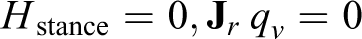

H_{stance} = 0, J_{r} q_{v} = 0

H_{stance} \in I R^{4}

contains the height of the four corners of the foot in contact with ground, and

J_{r} q_{v}

is the six elements vector with the linear and the angular velocity of the foot defined by equation (4).

E ₂: The four corners of the swing foot must follow the paths presented in Figure 4

P_{swing} = P_{swing}^{d}

P_{swing} \in I R^{12}

contains the Cartesian position of the four corners of the swing foot and

P_{swing}^{d}

is the desired path.

E ₃: The gait must be symmetrical with respect to the right and left legs. That means that the final configuration of the right leg must be equal to the initial configuration of the left leg. In the case of the Bioloid, this constraint implies the following equations

q_{7} (T) = - q_{8} (0), q_{8} (T) = - q_{7} (0)

q_{9} (T) = - q_{10} (0), q_{10} (T) = - q_{9} (0)

q_{11} (T) = - q_{12} (0), q_{12} (T) = - q_{11} (0)

q_{13} (T) = - q_{14} (0), q_{14} (T) = - q_{13} (0)

q_{15} (T) = - q_{16} (0), q_{16} (T) = - q_{15} (0)

q_{17} (T) = - q_{18} (0), q_{18} (T) = - q_{17} (0)

There are two main approaches to solving constrained optimization problems such as equation (8). One of them is using gradient-based methods, such as sequential quadratic programming, interior-point and trust-region-reflective. In these methods, when the gradient of the function to optimize is not available, it is approximated by finite differences. Nevertheless, in the case of the problems with a large number of variables, 60 in our case (12 trajectories with 5 parameters each), this approximation is computationally expensive and introduces numerical errors. The other approach is based on penalty-based methods⁴³ that turn constrained into unconstrained problems by introducing an artificial penalty for violating constraints. For example, the minimization of the function $100 / x$ subject to the constraint $x \leq 5$ can become an unconstrained optimization problem by adding a penalty function that returns a huge value when $x > 5$

min_{x} [\frac{100}{x} + α max {(0, x - 5)}^{2}]

The term $max (x - 5, 0)$ is equal to zero for $x \leq 5$ and equal to $α (x - 5)$ when $x > 5$ . In this way, if α is large enough, then no value of x that violates the constraint could be a minimum of the function 10.

The minimization of equation (8), subject to the previously defined constraints I ₁, I ₂, I ₃, E ₁, E ₂, and E ₃, was transformed in the following unconstrained problem

min_{θ} [J (θ) + P (q (θ), q_{v} (θ), q_{a} (θ))]

The vector $θ$ is composed by the coefficients of the truncated Fourier expansion defined by equation (9). The function $P (q (θ), q_{v} (θ), q_{a} (θ))$ is defined as follows

\begin{matrix} P (q (θ), q_{v} (θ), q_{a} (θ)) = P_{I} (q (θ), q_{v} (θ), q_{a} (θ)) \\ + P_{E} (q (θ), q_{v} (θ), q_{a} (θ)) \end{matrix}

where P_I and P_E are the penalty functions for the inequality and the equality constraints, respectively. To simplify notation, the arguments $q (θ)$ , $q_{v} (θ)$ , and $q_{a} (θ)$ will be omitted. The expression for P_I is given by equation (12)

P_{I} = α_{I} \sum_{k = 1}^{N_{I}} (e^{max (I_{k},0)} - 1)

If, for example, the inequality constraint k is $a \leq b$ , then I_k is defined as $a - b$ . When $I_{k} \leq 0$ , then the term $max (I_{k},0)$ is zero, and as a consequence $e^{max (I_{k},0)} - 1$ is also zero. When the inequality I_k is not satisfied, then its contribution to the penalty function P_I is $α_{I} (e^{I_{k}} - 1)$ . The expression for P_E is given by equation (13)

P_{E} = α_{E} \sum_{k = 1}^{N_{E}} (e^{max (|E_{k}| - Tol,0)} - 1)

If, for example, the equality constraint k is $a = b$ , then E_k is defined as $a - b$ . The constant $Tol$ is the tolerance for the equality conditions. When $| E_{k} | \leq Tol$ , then the term $e^{max (|E_{k}| - Tol,0)} - 1$ is also zero. When $| E_{k} | > Tol$ , then the contribution to the penalty function P_E is $α_{E} (e^{|E_{k}| - Tol} - 1)$ . Thus, the penalty-based optimization process requires a trial and error procedure to select $α_{I}$ , $α_{E}$ , and $Tol$ . The values used to calculate the optimal trajectories were $α_{I} {= 10}^{9}$ , $α_{E} {= 10}^{6}$ , and $Tol {= 10}^{- 3}$ .

As the purpose of using a penalty approach was to avoid gradient estimates, equation (11) was solved using Matlab’s fminsearch function, which is based on the Nelder–Mead simplex method.⁴⁴ The main criticism to this method is that no proof of convergence has been proposed. Nevertheless, we obtained better results using the penalty approach and fminsearch than using fmincon, which is the function for constrained optimization problems.

Experimental protocol

The comparison of the energy consumption between the cart-table and the optimization approaches is carried out at three different walking speeds: 0.5, 1.0, and 1.3 m/min. When the walking speed is greater than 1.3 m/min, the robot falls. This is because in our experimental setup, there is no closed-loop control that guarantees the balance of the robot. Energy consumption was recorded for 60 robot walks, 20 for each of the three walking speeds considered. For each speed, 10 walks were implemented using the cart-table approach, and the other $10$ using the optimization approach. In each trial, the robot walked in a flat and obstacle-free surface along a straight path 0.75 m long.

Results

The number of harmonics of equation (9) was selected by numerically solving the optimization problem (8) for different values of N. For $N = 1$ , no feasible solution was found. The values of the performance index (8) for N = 2–7 are presented in Table 5. For $N \geq 5$ , the addition of harmonics to equation (9) does not represent a significant decreasing of equation (8), and by consequence we selected $N = 5$ .

Table 5.

The performance index described by equation (8) as a function of the number of harmonics used to describe the joint trajectories.

N	Performance equation (8)
2	0.2017
3	0.1179
4	0.1026
5	0.1035
6	0.1029
7	0.1026

From Table 6, it can be seen that for all joints the range of motion for the optimization method is smaller than that obtained with the cart-table approach.

Table 6.

Range of motion for each of the robot joints.^a

Joint	Plane	Cart-table	Optimization
Right hip	CP	36.47°	1.23°
Right hip	SP	43.82°	38.49°
Right knee	SP	75.65°	57.23°
Right ankle	SP	34.77°	30.16°
Right ankle	CP	36.47°	1.23°

CP: coronal plane; SP: sagittal plane.

^a As the gait is symmetric with respect to the legs, only the values for the right leg are presented.

The joint trajectories for the cart-table and the optimization methods are presented in Figures 5 and 6.

Figure 5.

Hip trajectories for the cart-table (blue) and the optimization (red) methods. TP: transversal plane; CP: coronal plane; SP: sagittal plane.

Figure 6.

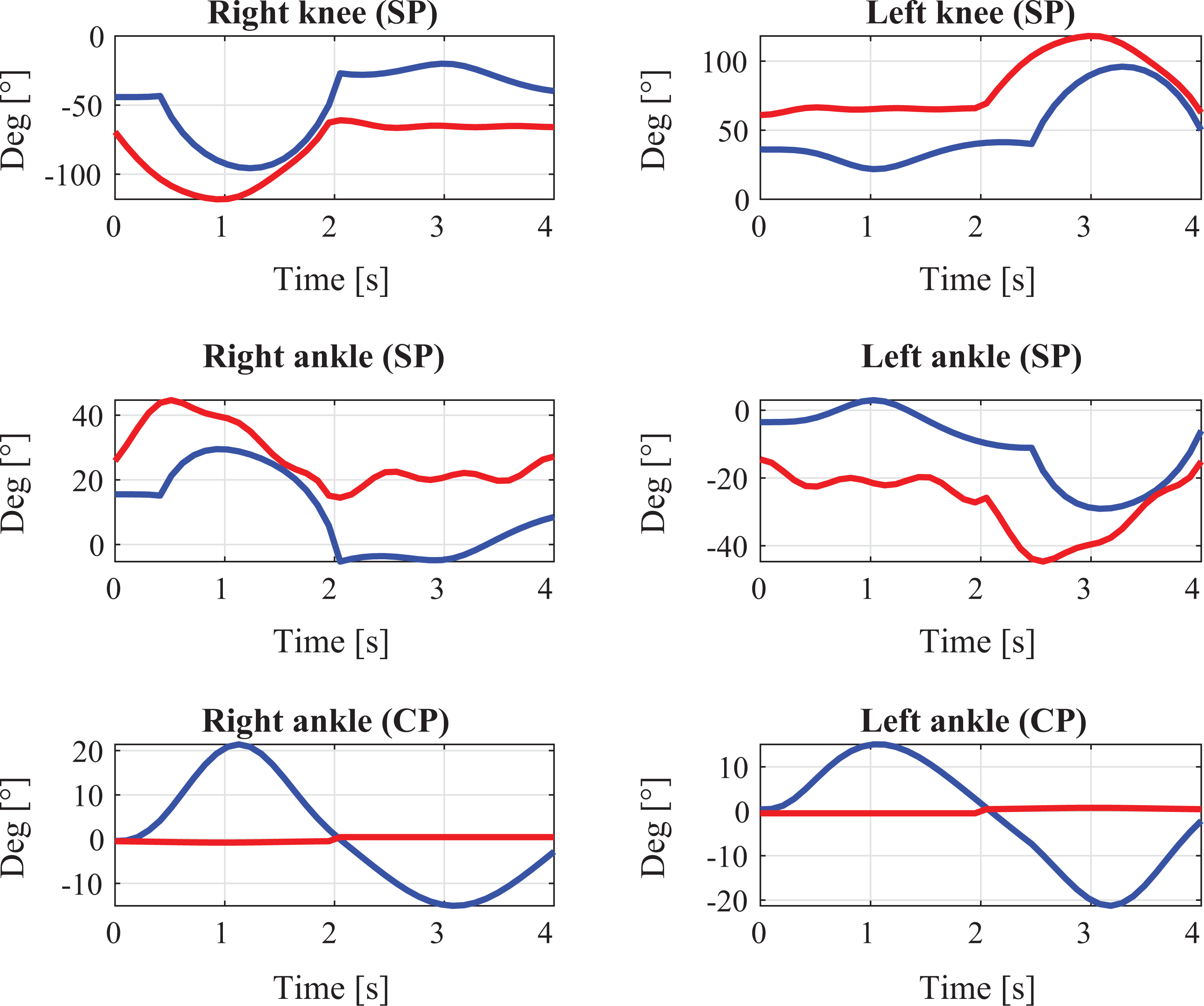
Knee and ankle trajectories for the cart-table (blue) and the optimization (red) methods. TP: transversal plane; CP: coronal plane; SP: sagittal plane.

The energy consumption for the 60 trials is presented in Table 7. The last row of this table contains the cost of transportation (COT), which is calculated considering a mass of 1.7 kg and a distance of 0.75 m. From Figure 7, it can be seen that for the three considered speeds, the median of the energy consumption was lower for the optimization approach. At a speed of 0.5 m/min, the average energy for the optimization approach was 88.22% of the average energy for the cart-table method. For the other two speeds, these values were 91.61% (to 1.0 m/min) and 90.98% (to 1.3 m/min). Statistical analysis of experimental data can be performed using parametric or nonparametric methods. The former applies only when the data are normally distributed, and the latter does not require this assumption. The parametric method for comparing the means of two data sets is the Student’s test, and its nonparametric equivalent is the Wilcoxon test. However, the Wilcoxon test does not compare means but medians.

Table 7.

Energy consumption in Joules for the cart-table and the optimization approaches at different speeds.^a

	Speed 0.5 m/min		Speed 1.0 m/min		Speed 1.3 m/min
Trial	Cart-table	Optimization	Cart-table	Optimization	Cart-table	Optimization
1	778	673	382	318	525	439
2	769	743	370	353	516	432
3	941	781	392	333	494	430
4	922	701	382	330	480	424
5	843	787	364	348	488	430
6	843	782	365	325	503	435
7	914	785	364	299	495	458
8	866	751	369	364	474	497
9	791	745	351	388	500	501
10	785	707	343	315	473	457
Mean	845	745	368	337	494	450
COV	7.60%	5.39%	3.96%	7.74%	3.46%	6.25%
COT	72.39	63.86	31.53	28.88	42.38	38.56

^a COT stands for cost of transportation, and COV for coefficient of variation, which is the standard deviation divided by the mean.

Figure 7.

Energy consumption for the cart-table (CT) and the optimization (Opt) approaches at three different walking speeds (0.5, 1.0, and 1.5 m/min).

The Jarque–Bera test for normality was applied to the six data sets collected during the experiments (two trajectory generation methods and three gait speeds), and the results indicated that some of them are normally distributed but others are not. As a consequence, a nonparametric approach was used. The Wilcoxon test was applied to verify if the differences in energy consumption were significant. At each speed, the research hypothesis was that the energy consumption for the trajectory generated with the optimization approach was lower than that obtained by applying the cart-table method. By using the ranksum function of Matlab, the resulting p values were $p < 0.001$ for 0.5 m/min, $p = 0.0034$ for 1.0 m/min, and $p = 0.0019$ for 1.3 m/min. Figure 4 shows the joint angles as a function of time, for the two applied joint trajectory generation approaches, and considering a walking speed of 1 m/min.

Discussion

The cost of transportation

During the experiments, we do not use the stabilizing mechanism provided by the gyroscope of the robot to avoid the corrections it introduces in the joint trajectories. In this manner, we compare the electrical energy expenditure of the original gaits generated by each method (cart-table and optimization) without introducing any bias in the experiment. Nevertheless, the main drawback of this open-loop motion is that the maximal gait velocity attained by the robot is only 1.3 m/min. Above this value, the robot falls at each trail. The consequence of the low gait speeds is the high COT we obtain for the Bioloid, which ranged from 28.88 to 72.39, depending on the gait speed and the trajectory generation approach. These values are by far greater than those reported for similar robots. For NAO,¹⁸ the COT ranges between 2.4 and 5.8, and for the DARwIn-OP,³⁵ from 1.5 to 9.0. The high COT we obtain for the Bioloid is caused by the low gait speeds used during the experiments. The high energy consumption at low velocities has been reported for both humans and robots. In their study, Roberts et al.³⁵ present experimental results where the energy consumption at 0.025 m/s was nine times higher than that at 0.15 m/s.

Another reason explaining the high COT obtained is the compliance margin and slope of the servomotors, which were configured to their maximal values to guarantee a precise tracking of the reference trajectory. Nevertheless, the higher the stiffness, the greater the current consumption. For example, in the case of the robot Aldebaran-NAO,¹⁸ the experimental results show that the current supplied by the battery is almost double when the stiffness was changed from its minimum value to the maximum.

The sources of variability

The coefficient of variation (COV) of the COT takes values between 3.46% and 7.60% (see the row COV in Table 7). This is because during the experimentation we could not guarantee that the robot would walk on a perfect straight path, and as a consequence, the distance traveled by the robot was different from 0.75 m. Our COVs are consistent with those reported in similar experiments. In their study, Roberts et al.³⁵ reported COVs ranging from 5.9% to 12.4% for the energy expenditure of the DARwIn-OP humanoid robot. In the study by Ogura et al.,⁴⁵ the electrical energy expenditure of the WABIAN robot is measured for three walking styles and two different step lengths (a total of six experimental configurations). The walking patterns were generated using a zero-moment-point-based approach, and the difference between gait styles lay in the trajectories of the knees. Only one trial was made for each gait, and as a consequence, it is difficult to assess whether the differences in energy consumption were statistically significant or not.

The benefits of the optimization

In the study of Bhounsule et al.,⁴⁶ an optimization based on the dynamic model of the four-legged robot Ranger was used to generate its gait trajectory. This approach led to a reduction in the total COT from 0.28 to 0.19, when compared with trajectories intuitively tuned. This reduction of 32.14% is larger than that obtained in our experiments, which ranged from 9.16% to 13.35%. We hypothesized that these differences are due to the optimization approach. In their study, Bhounsule et al.⁴⁶ optimize the control signal applied to the robot, and in our case, the parameters used to describe the trajectory as a function of time.

The experimental results presented in this article show that for the three considered walking speeds, the average energy consumption obtained by applying the optimization approach is lower than that obtained with the cart-table method. From the results presented in Table 6, it can be seen that the main reason for these differences is the range of joint motion, which for the cart-table approach is always greater than that obtained by optimization. For the knee, a joint that can be an important source of energy consumption,^45,47 the optimization reduces the range of motion to 75.65% of the value obtained by the cart-table method.

The results of Wilcoxon test show that in all cases the differences are not due to chance but to the method used to generate the joint trajectories. To the best of our knowledge, an experimental comparison of electrical energy consumption between the cart-table and the optimization approaches has not been reported elsewhere.

Despite the encouraging results presented in this article, the optimization approach has some disadvantages when compared with the cart-table method. One of them is the high computational cost associated with solving the minimization problem described by equation (8). In the case of the trajectories presented here, 3–6 h of calculations were required on a laptop CORE-I7 with 32 GB of RAM to find a local minimum (the calculation time depended largely on the walking speed). Nevertheless, the main barrier to the adoption of the optimization approach is the need for a dynamic model of the robot, which is a procedure that requires vast experience and is prone to errors.

It is important to clarify that the limitation in the maximal velocity reduces the generality of our results. This is because the minimization of equation (8) implies the minimization of the electrical energy expenditure only when the relationship between the joint torques and the current supplied to the actuators is linear. When the joint velocities are increased, the equation that relates these two variables could become nonlinear, for example, due to magnetic saturation,⁴⁸ and consequently, the minimization of equation (8) does not guarantee energy expenditure minimization. In such a case, it could not be ensured that the optimal trajectories lead to a less energy expenditure than the cart-table approach.

Future work

The electronic system presented in Figure 3 measures the energy expenditure of a given trajectory. Thanks to this system, we conclude that a trajectory minimizing the square torques leads to a lower energy expenditure than a trajectory generated by using the cart-table method. Nevertheless, for future works, we need to develop a current and voltage measurement system for each of the actuators to know which joints have the highest energy expenditure. In addition, we want to experimentally compare energy expenditure for innovative techniques for the generation of trajectories in biped robots such as the divergent component of motion⁴⁹ and the essential model.⁵⁰

Conclusion

The optimization approach requires a full mathematical model describing the dynamics of the biped. In practice, this model is just an approximation of the actual dynamic of the robot, neglecting the dynamics of the actuators and using an oversimplified representation of friction phenomena. Despite these limitations, the optimization approach leads to an important saving in energy consumption for low gait speeds.

Footnotes

Acknowledgement

The authors would like to recognize and express their sincere gratitude to Universidad del Cauca (UNICAUCA), Colombia, for the financial support granted during this project.

Declaration of conflicting interests

The author(s) declared no potential conflicts of interest with respect to the research, authorship, and/or publication of this article.

Funding

The author(s) disclosed receipt of the following financial support for the research, authorship, and/or publication of this article: This work was financially supported by Universidad del Cauca (UNICAUCA), Colombia ( $501100005682$ ).

ORCID iD

Diego Bravo

References

Scalera

Palomba

Wehrle

, et al. Natural motion for energy saving in robotic and mechatronic systems. Appl Sci 2019; 17(9): 3516.

Woolfrey

Liu

. A control method for joint torque minimization of redundant manipulators handling large external forces. J Intell Robot Syst 2019; 96(1): 3–16.

Trigatti

Boscariol

Scalera

, et al. A new path-constrained trajectory planning strategy for spray painting robots—rev.1. Int J Adv Manuf Techol 2018; 98(9): 2287–2296.

Singh

Dutta

Saxena

. Design of a biped robot with torsion springs at the joints for reduced energy consumption during walk. In: ASME 2009 international design engineering technical conferences and computers and information in engineering conference, San Diego, California, 30 August–2 September 2009, pp. 987–992. DOI: 10.1115/DETC2009-86595.

Rengifo

Kaddar

Aoustin

, et al. Reactive power compensation in mechanical systems. In: International conference on multibody dynamics, Stuttgart, Germany, 29 May–1 June 2012.

Chew

Choong

Poo

, et al. From science fiction to reality—humanoid robots. In: First humanoid, nanotechnology, information technology, communication and control, environment and management (HNICEM) international conference, Manila, Philippines, 27–30 March 2003.

Ogino

. Embodiment approaches to humanoid behavior—energy efficient walking and visuo-motor mapping. PhD Thesis, Osaka University, Japan, 2005.

Rivas

Cañas

González

. Aprendizaje automático de modos de caminar para un robot humanoide. In: Proceedings of the 6th international conference on human-robot interaction.

Dai

Valenzuela

Tedrake

. Whole-body motion planning with centroidal dynamics and full kinematics. In: 2014 IEEE-RAS international conference on humanoid robots, Madrid, Spain, 18–20 November 2014, pp. 295–302. IEEE. DOI: 10.1109/HUMANOIDS.2014.7041375.

10.

Kajita

Kanehiro

Kaneko

, et al. Biped walking pattern generation by using preview control of zero-moment point. In: 2003 IEEE international conference on robotics and automation (Cat. No. 03CH37422), Taipei, Taiwan, 14–19 September 2003, vol. 2, pp. 1620–1626. IEEE. DOI: 10.1109/ROBOT.2003.1241826.

11.

Kajita

Morisawa

Harada

, et al. Biped walking pattern generator allowing auxiliary ZMP control. In: 2006 IEEE/RSJ international conference on intelligent robots and systems, Beijing, China, 9–15 October 2006, pp. 2993–2999. IEEE. DOI: 10.1109/IROS.2006.282233.

12.

Sakagami

Watanabe

Aoyama

, et al. The intelligent ASIMO: system overview and integration. In: IEEE/RSJ international conference on intelligent robots and systems, Lausanne, Switzerland, 30 September–4 October 2002, vol. 3, pp. 2478–2483. IEEE. DOI: 10.1109/IRDS.2002.1041641.

13.

Chestnutt

Lau

Cheung

, et al. Footstep planning for the Honda ASIMO humanoid. In: Proceedings of the 2005 IEEE international conference on robotics and automation, Barcelona, Spain, 18–22 April 2005, pp. 629–634. IEEE. DOI: 10.1109/ROBOT.2005.1570188.

14.

Kaneko

Kanehiro

Kajita

, et al. Humanoid robot HRP-2. In: Proceedings of the IEEE international conference on robotics and automation, 2004, ICRA ‘04, New Orleans, LA, 26 April–1 May 2004, vol. 2, pp. 1083–1090. IEEE. DOI: 10.1109/ROBOT.2004.1307969.

15.

Kaneko

Harada

Kanehiro

, et al. Humanoid robot HRP-3. In: 2008 IEEE/RSJ international conference on intelligent robots and systems, Nice, France, 22–26 September 2008, pp. 2471–2478. IEEE. DOI: 10.1109/IROS.2008.4650604.

16.

Kaneko

Kanehiro

Morisawa

, et al. Humanoid robot HRP-4—humanoid robotics platform with lightweight and slim body. In: 2011 IEEE/RSJ international conference on intelligent robots and systems, San Francisco, CA, 25–30 September 2011, pp. 4400–4407. IEEE. DOI:10.1109/IROS.2011.6094465.

17.

Aldebaran Robotics. User guide and technical guide for NAO robot. Technical report, 2017.

18.

Kulk

Welsh

. A low power walk for the NAO robot. In: Proceedings of the Australasian conference on robotics and automation (ACRA), Canberra, Australia, 2008, pp.1-7.

19.

Park

Kim

Lee

, et al. Mechanical design of the humanoid robot platform, HUBO. Adv Robot 2007; 21(11): 1305–1322.

20.

Atmeh

Ranatunga

Popa

, et al. Implementation of an adaptive, model free, learning controller on the Atlas robot. In: 2014 American control conference, Portland OR, 4–6 June 2014, pp. 2887–2892. IEEE. DOI: 10.1109/ACC.2014.6859431.

21.

Feng

Whitman

Xinjilefu

, et al. Optimization based full body control for the Atlas robot. In: 2014 IEEE-RAS international conference on humanoid robots, Madrid, Spain, 18–20 November 2014, pp. 120–127. IEEE. DOI: 10.1109/HUMANOIDS.2014.7041347.

22.

Chevallereau

Aoustin

. Optimal reference trajectories for walking and running of a biped robot. Robotica 2001; 19: 557–569.

23.

Saidouni

. Numerical synthesis of three-dimensional gait cycles by dynamics optimization. Robotica 2011; 29(3): 445–459.

24.

Grizzle

Chevallereau

Sinnet

, et al. Models, feedback control, and open problems of 3D bipedal robotic walking. Automatica 2014; 50(8): 1955–1988.

25.

Ahmed

Aris

Marhaban

, et al. Power consumption rate analysis of Bioloid humanoid robot: towards energy saving and source development. In: 2015 10th Asian control conference (ASCC), Kota Kinabalu, Malaysia, 31 May–3 June 2015, pp. 1–6. IEEE. DOI: 10.1109/ASCC.2015.7244843.

26.

Aoustin

. Walking gait of a biped with a wearable walking assist device. Int J Hum Robot 2015; 12(4): 1550018.

27.

Tlalolini

Aoustin

Chevallereau

. Human-like walking: optimal motion of a bipedal robot with toe-rotation motion. IEEE/ASME Trans Mechatron 2011; 16(2): 310–320.

28.

Schiehlen

. Energy-optimal design of walking machines. Multibody Syst Dyn 2005; 13(1): 129–141.

29.

Tlalolini

Aoustin

Chevallereau

. Design of a walking cyclic gait with single support phases and impacts for the locomotor system of a thirteen-link 3D biped using the parametric optimization. Multibody Syst Dyn 2009; 23(1): 33.

30.

Shugen

Watanabe

. Time optimal control of kinematically redundant manipulators with limit heat characteristics of actuators. In: Proceedings of 2001 IEEE/RSJ international conference on intelligent robots and systems. Expanding the societal role of robotics in the next millennium, Maui, HI, 29 October–3 November 2001, vol. 1, pp. 152–157. IEEE. DOI: 10.1109/IROS.2001.973351.

31.

Shin

Kim

. Energy-efficient gait planning and control for biped robots utilizing vertical body motion and allowable ZMP region. IEEE Trans Ind Electron 2015; 62(4): 2277–2286.

32.

Roussel

de Wit

Goswami

. Generation of energy optimal complete gait cycles for biped robots. In: Proceedings of 1998 IEEE international conference on robotics and automation (Cat. No. 98CH36146), Leuven, Belgium, 20 May 1998, vol. 3, pp. 2036–2041. IEEE.

33.

Huang

Hase

. Energy-efficient trajectory planning for biped walking robot. In: 2006 IEEE international conference on robotics and biomimetics, Kunming, China, 17–20 December 2006, pp. 648–653. IEEE. DOI: 10.1109/ROBIO.2006.340283.

34.

Tlalolini

Chevallereau

Aoustin

. Comparison of different gaits with rotation of the feet for a planar biped. Robot Auton Syst 2009; 57(4): 371–383.

35.

Roberts

Quacinella

Kim

. Energy expenditure of a biped walking robot: instantaneous and degree-of-freedom-based instrumentation with human gait implications. Robotica 2017; 35(5): 1054–1071.

36.

Luh

JYS

Walker

Paul

RPC

. On-line computational scheme for mechanical manipulators. J Dyn Syst Meas Control 1980; 102(2): 69–76.

37.

Khalil

Dombre

. Modeling, identification and control of robots. 2nd ed. Paris, France: Butterworth-Heinemann, 2004.

38.

Regan

Munson

Zimmer

, et al. Current sense circuit collection. Technical report, Linear Technology Corporation, 2005.

39.

Vukobratovic

Branislav

. Zero-moment point—thirty five years of its life. Int J Hum Robot 2004; 1: 157–173.

40.

Al-Shuka

HFN

Corves

Hong Zhu

, et al. A simple algorithm for generating stable biped walking patterns. Int J Comput Appl 2014; 101(4): 29–33.

41.

Samadi

Moghadam-Fard

. Pattern generation for humanoid robot with natural ZMP trajectory. In: 2014 second RSI/ISM international conference on robotics and mechatronics (ICRoM), Tehran, Iran, 15–17 October 2014, pp. 570–575. IEEE.

42.

Rioja

UAJ

. Equilibrio dinámico de un robot bípedo utilizando el modelo simplificado carro-mesa. Technical report, Universidad Nacional Autónoma de México, 2014.

43.

Polyakova

Karelin

. Exact penalty methods for nonsmooth optimization. In: 2014 20th international workshop on beam dynamics and optimization (BDO), St. Petersburg, Russia, 30 June–4 July 2014, pp. 1–2. IEEE. DOI: 10.1109/BDO.2014.6890067.

44.

Nelder

Mead

. A simplex method for function minimization. Comput J 1965; 7(4): 308–313.

45.

Ogura

Kataoka

Aikawa

, et al. Evaluation of various walking patterns of biped humanoid robot. In: Proceedings of the 2005 IEEE international conference on robotics and automation, Barcelona, Spain, 18–22 April 2005, pp. 603–608. IEEE. DOI: 10.1109/ROBOT.2005.1570184.

46.

Bhounsule

Cortell

Grewal

, et al. Low-bandwidth reflex-based control for lower power walking: 65 km on a single battery charge. Int J Robot Res 2014; 33(10): 1305–1321.

47.

Kim

Park

. Realization of stretch-legged walking of the humanoid robot. In: 8th IEEE-RAS international conference on humanoid robots, Daejeon, South Korea, 1–3 December 2008, pp. 118–124. IEEE. DOI: 10.1109/ICHR.2008.4755941.

48.

Bermingham

O’Donovan

Walsh

, et al. Optimized control of high-performance servo-motor drives in the field-weakening region. In: 2016 IEEE applied power electronics conference and exposition (APEC), Long Beach, CA, 20–24 March 2016, pp. 2794–2800. IEEE. DOI: 10.1109/APEC.2016.7468260.

49.

Englsberger

Ott

Albu-Schäffer

. Three-dimensional bipedal walking control using divergent component of motion. In: 2013 IEEE/RSJ international conference on intelligent robots and systems, Tokyo, Japan, 3–7 November 2013, pp. 2600–2607. IEEE. DOI: 10.1109/IROS.2013.6696723.

50.

De-León-Gómez

Luo

Kalouguine

, et al. An essential model for generating walking motions for humanoid robots. Robot Auton Syst 2019; 112: 229–243.

An experimental energy consumption comparison between trajectories generated by using the cart-table model and an optimization approach for the Bioloid robot

Abstract

Keywords

Introduction

Bioloid robot

CAD model

Dynamic model of the robot

Materials and methods

Energy expenditure measurement system

Joint trajectory convention

Trajectory generation using the cart-table approach

Trajectory generation using the optimization approach

Experimental protocol

Results

Discussion

The cost of transportation

The sources of variability

The benefits of the optimization

Future work

Conclusion

Footnotes

Acknowledgement

Declaration of conflicting interests

Funding

ORCID iD

References