Sage Journals: Discover world-class research

Abstract

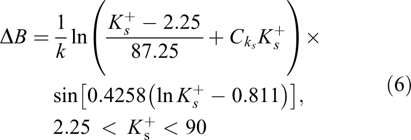
Through numerical calculations, it could be found that when the blade surface quality reaches a certain level, the surface quality of the blade was continuously improved, and the guarantee effect on its performance would be weakened. Under this circumstance, continuing to improve the surface quality of the blade had no positive effect on the performance of the blade. Studies had shown that when the blade surface equivalent grit roughness K_s reaches 4.96 (about R _a = 0.8 µm), the blade performance was close to the smooth surface of the blade, and no further processing was required to improve the surface roughness. When the surface equivalent grit K_s was greater than 4.96 µm, the surface roughness had a great influence on the blade performance. When K_s was larger than 40 µm, the negative effect is significantly increased. For the different characteristics of the blade and different processing conditions, four kinds of robot-based blade surface grinding schemes were proposed, of which the core content was the robot layout. Based on the robot group’s fitting to the spatial surface and the path planning, the experimental verification was carried out.

Keywords

Engine blade surface machining robot processing surface roughness measurement blade performance evaluation

Introduction

Before the final finishing of the blade, its surface roughness and positional accuracy of the key parts do not meet the design requirements, and even if the blade has reached the design requirements after processing, it will change due to high temperature and high pressure or other harsh conditions. It is rough or partially deformed, so that the design performance of the blade is not achieved. Assembling the unmachined blades into the engine will affect the working state of the aeroengine. The main performances are the engine’s thrust-to-weight ratio and the stable working range of the engine will be reduced, which can greatly reduce the efficiency of the aircraft engine and also can bring hidden dangers for safe navigation.

Using blades that have not been finished for the engine will result in a loss of engine performance, which is a result that has become a consensus in the aerospace industry. Research in this field was began in the late 1970s, when Bammert and Sandstede,¹ professors at Gottfried Wilhelm Leibniz Universität Hannover in Germany, conducted a study based on turbine cascades, which used experimental methods to determine the chord length of the blade and so on. Theoretically exploring and attempting to numerically study was carried out in the 1990s. According to the theory, the variables of aero-engine blade performance caused by changes in surface roughness were quantitatively and meticulously studied. It is a rare influence on the influence of the key performance factors of the blade. The research results of this influence mechanism can be directly applied to the engineering practice of blade manufacturing, which can guide the setting of the level precision requirements of blade processing, and can guide the development of standards for the maintenance of old blades. Studying the influence of aero-engine blade surface topography on blade performance will have great positive significance for engine blade design and processing, especially for the quantitative assessment of engine blade finishing.

Engine blade machining accuracy is affected by many factors, and there will be interference factors such as force deformation, heat deformation, and vibration deformation. To minimize the interference of these factors, the relevant manufacturing fields generally use various methods such as forging, precision casting, milling, manual grinding, and rough-to-finish machining methods. First, the blade blank is obtained by precision casting (wax casting) or precision forging (die forging) and other methods,^2

–7 followed by machining for the purpose of finishing. After the polishing by polishing and grinding tools such as abrasive belts, pneumatic pressure wheels, and louvers wheel,^8,9 the surface margin of the blades and casting defects are removed, and the surface accuracy of the blades meets the design requirements. Due to the lack of special machine tool processing equipment, many blades are still finished by manual grinding and polishing.^10
–12

The emergence of NC (numerical control) milling technology has provided a new way for the manufacture of blades. However, when milling thin-walled blades, it is more obvious due to vibration and other phenomena, and deformation is difficult to control during processing, which affects the blade machining accuracy. The quality of the parts is difficult to guarantee. In the “Aeronautical Manufacturing Engineering Manual” published at the beginning of the 21st century, milling of blades has not yet been listed as a common method of blade manufacturing. Due to the existence of the milling texture, the blade must be surface-finished to meet the design requirements, but the consistency of the manually polished blades is poor, which adversely affects the dynamic balance of the shaft system, and the manual polishing method is inefficient and easy to appear on the blade surface Ablation increases scrap rates and manufacturing costs. Based on the above reasons, this article will study the blade surface performance and its robotic machining.

Blade surface roughness model

Wall function correction

As the airflow flows through the surface of the non-smooth blade, its various physical properties and its motion state will change. The aerospace industry practitioners have long recognized that the tiny surface of the blade surface affects the surface of the blade. Factors such as resistance, heat transfer, and mass transport capacity should be considered when studying the characteristics of the blade, for example, the influence of wall roughness on the calculation of the turbulent flow simulation with wall roughness limitation. It cannot be ignored. In this article, the influence of the precision of the machining on the blade performance is studied by setting different blade surface wall roughness.

In general, when studying the wall properties of non-smooth surfaces, an expandable wall function¹³ can be used to express the airflow velocity near the wall of the blade, namely

u^{*} = \{\begin{matrix} y^{*}, \begin{matrix}  \end{matrix} y^{*} < 11.25 \\ \frac{1}{k} ln (C^{RH} y^{*}), y^{*} \geq 11.25 \end{matrix}

In the above formula, k is the Von Karman constant, generally taken as k = 0.42, C ^RH is the wall roughness coefficient, y* is the dimensionless distance of the airflow to the blade wall surface, and

y^{*} = \frac{ρ u_{τ} y_{p}}{μ}

y_p in the above formula is the vertical distance from the point p to the wall surface, and $u_{τ}$ is the square root of the ratio of the turbulent shear stress to the air density. It has a velocity dimension and is called a friction velocity. Its expression is given as

u_{τ} = \sqrt{\frac{τ_{ω}}{ρ}}

The near wall velocity function described above is suitable for the analysis of an approximately smooth blade surface. When the blade is from the blank surface to the near smooth surface, the span of the surface roughness is large. In this case, formula (2) is used. The calculation method of formula (1) will lead to drastic fluctuations in wall shear stress and heat transfer coefficient, resulting in an increase in analysis error. Therefore, this article uses the following method to modify the wall speed function, namely

u^{*} = \frac{1}{k} ln (C^{RH} \frac{ρ y^{*}}{μ}) - Δ B

$Δ B$ in the above formula is a wall surface roughness function, which limits the transition of the cutoff point of the average velocity distribution of the near-wall fluid due to the influence of roughness, and is an important factor for measuring the transition of the cutoff point. It is generally believed that the expression of $Δ B$ depends on the type and size of the wall roughness, such as a sand surface, a threaded surface, a rivet surface, and a wire mesh surface. Admittedly, various types of surface roughness correspond to various types of wall surface roughness functions, so $Δ B$ does not have a clear and uniform common equation. Through a series of experiments, $Δ B$ of the sand-like surface has relationship to the roughness-free mass value $K_{S}^{+}$ , and it can be considered that $Δ B$ is a multi-valued function of the dimensionless value $K_{S}^{+}$ . Due to the difference of $K_{S}^{+}$ , the wall can be divided into the following three types:

liquid dynamic smooth zone, $K_{S}^{+} \in (0, 5)$ ;

transition zone, $K_{S}^{+} \in (5, 90)$ ; and

completely rough zone, $K_{S}^{+} \in (90, \infty)$ .

If the surface of the blade is very close to smooth, the effect of surface roughness on the performance of the blade will be negligible. If the surface of the blade is the surface roughness in the form of a transition zone, the effect of its surface roughness on its performance will be important. Significantly, if the surface of the blade is completely in the state of the blank and is completely rough, the influence of its surface roughness on its performance is very important and significant.

For the wall law of the near-wall fluid velocity distribution described above, Cebeci and Bradshaw proposed an empirical expression based on Nikuradse’s data, namely

Δ B = 0, \begin{matrix} K_{s}^{+} \end{matrix} < 2.25

\begin{array}{l} Δ B = \frac{1}{k} ln (\frac{K_{s}^{+} - 2.25}{87.25} + C_{k_{s}} K_{s}^{+}) \times \\ sin [0.4258 (ln K_{s}^{+} - 0.811)], \\ 2.25 < K_{s}^{+} < 90 \end{array}

Δ B = \frac{1}{k} ln (1 + C_{k_{s}} K_{s}^{+}), K_{s}^{+} > 90

$C_{k_{s}}$ in the above formula is a roughness constant, and its value is determined by the type of rough surface. It can be seen from the above discussion that in the model wall framework, the roughness wall simulation study requires two parameters, namely, the roughness height $K_{s}$ and the roughness constant $C_{k_{s}}$ .

Researchers in related fields have studied the surface displacement of the gravel surface.^14

–17 The grit volume model can be selected for the surface topography. This size model can be expressed by $K_{s}$ , which can be used as follows

K_{s}^{+} = \frac{K_{s} \sqrt{ρ τ_{w}}}{μ}

and

K_{s} = 6.2 R_{a}

In the above formula, R _a is the processing roughness of the blade surface.

For uniform rough roughness avoidance, the roughness height can be approximated as $K_{s}$ , but when the surface roughness is not uniform, or is similar to other surface roughness such as barbed wire, except for formula (8). In addition to the appropriate roughness height $K_{s}$ , it is also necessary to adjust the appropriate roughness constant $C_{k_{s}}$ , and related experiments have shown^18,19 for nonuniform surface roughness, ribbed surface, and wire mesh on the surface, when the roughness constant $C_{k_{s}}$ is selected from 0.5 to 1, and the Nikuradse’ resistance data can be well simulated and reproduced.

Governing equation of near-wall airflow

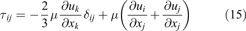
For transonic aero-engine blades, the high-speed gas between the cascades during operation is a viscous compressible gas stream, then

c_{v} = \frac{R}{γ - 1}

e = c_{v} T = \frac{P}{(γ - 1) ρ}

In the above two formulas, R is the gas constant, γ is the specific heat ratio of the fluid, and for air, γ is 1.4, e is the internal energy of the unit fluid, T is the temperature of the fluid, and ρ is the density of the fluid.

The mass conservation equation, the momentum conservation equation, and the energy conservation equation for the above fluids are

\frac{\partial P}{\partial t} + \nabla • (ρ \vec{v}) = 0

\frac{\partial}{\partial t} (ρ \vec{v}) + \nabla • (ρ \vec{v} \vec{v}) + \nabla (- P I^{e} + Γ)

\frac{\partial}{\partial t} (ρ E) + \nabla • (ρ \vec{v} E) = \nabla • [(- P I^{e} + Γ) • \vec{v}] - \nabla • \vec{q}

I^e in the above formula is a unit tensor, which can be expressed in the form $I^{e} = \{δ_{ij}\}$ ; $Γ$ is the viscous stress tensor, written as $Γ = \{τ_{ij}\}$ in the similar unit tensor form, for the airflow between the blades, that is, Newtonian fluid; and $τ_{ij}$ can be used expressed as follows

τ_{i j} = - \frac{2}{3} μ \frac{\partial u_{k}}{\partial x_{k}} δ_{i j} + μ (\frac{\partial u_{i}}{\partial x_{j}} + \frac{\partial u_{j}}{\partial x_{j}})

$\vec{q}$ is the heat flux density vector, that is, $\vec{q} = \{q_{i}\}$ , and the airflow near the blade wall follows the Fourier heat conduction law, so its expression can be $\vec{q} = K \nabla • T$ .

In the above formulas, $\vec{v}$ is the fluid velocity vector, K is the fluid heat transfer coefficient, T is the system fluid temperature, and E^e is the total energy per unit fluid near the blade wall surface. The expression is

E^{e} = e + \frac{1}{2} \vec{v} • \vec{v}

The relationship between gas pressure and density can be used to correlate the above equations, that is, $P = ρ R T$ ; in addition, the viscosity coefficient $μ$ of the gas fluid is related to the temperature T of the fluid; and the relationship between the two can be expressed by the Sutherland empirical formula, which is

\frac{μ (T)}{μ_{0}} = {(\frac{T}{T_{0}})}^{\frac{3}{2}} \frac{(T_{0} + T_{S})}{(T + T_{S})}

In the above formula, T _s is the Sutherland constant. If the fluid to be studied is air, the value can be taken as $T_{s} = 110.55 K$ , and $T_{0} = 293.15 K$ . $μ_{0}$ is the viscosity coefficient of the fluid under study at temperature $T_{0} = 293.15 K$ , and its value is $μ_{0} = 1.716 \times 10^{- 5} Pa \cdot s$ .²⁰

The calculation of the influence of blade surface roughness is based on CFX 17.0 software. As analyzed in the previous section, the surface roughness of the dimension-less factor Ks of the equivalent grit roughness model can be used to perform the movement case of the gas stream near the blade surface for different blade surface roughness. In the case of the blade, the movement of the gas stream near the surface of the blade. The relationship between the average surface roughness R_a and $K_{s}$ of the pressure and suction surfaces of the engine blades (or the blade back and the basin) is the Koch and Smith’s empirical model: $K_{s} = 6.2 R_{a}$ . The above empirical model also establishes a “rough wall Reynolds number” associated with the surface roughness of the blade,^21,22 namely

{Re}_{k} = \frac{k_{s} W_{in}}{μ_{ν}}

The above formula is used to determine whether the surface of the blade component is hydraulically smooth or rough. In the above formula, $W_{in}$ is the relative velocity of the fluid at the inlet of the runner, and $μ_{ν}$ is the dynamic viscosity coefficient of the airflow in this region. The dividing line, when the Reynolds value of the rough wall is greater than 90, the wall is rough, and when the value is less than 90, the influence of the surface roughness on the fluid motion in the vicinity can be neglected.

Machining accuracy and performance of blade surface

Model of blade cross section

As shown in Figure 1, the research in this article uses the planar cascade of the second-stage guide blade of an advanced aeroengine as the research object. To ensure that the numerical simulation can reflect the real blade working state, it must be set accurately and in accordance boundary condition to meet the blade working condition. The boundary condition of the working condition, the inflow of the guide vane is not along the normal direction of the hub plane, and the airflow speed and direction according to the actual situation must be set. Such numerical simulation can show the guiding significance of the actual machining. First, the airflow at the exit of the blade of the previous stage has an axial velocity c ₁, the axial velocity of the rotating impeller is reduced by the high-speed airflow of the rotating impeller, and the direction of motion of the rotating blade (moving at the linear velocity u ₂ in the rotational tangential direction) is obtained. The tangential velocity, after passing through the guide vanes, is directed to the axial direction, the velocity is reduced, and the pressure is increased, thus completing the compression process of the primary vane to the airflow.

Figure 1.

Schematic diagram of the engine low-pressure compressor blade.

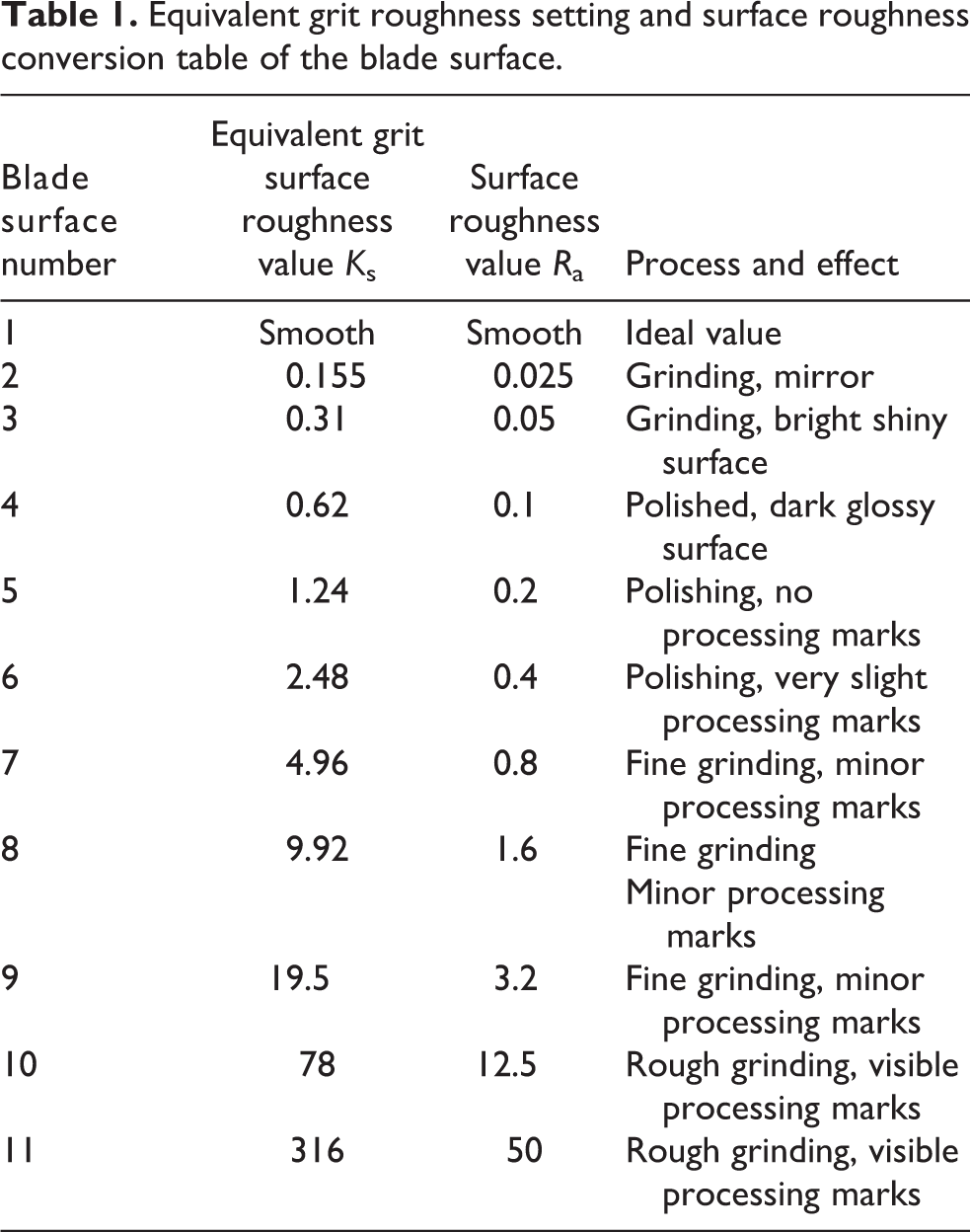
In this article, the Mach number and pressure distribution in the guide blade cascade channel with different surface roughness at low flow rate are investigated. Table 1 presents the roughness value of the blade surface. Figure 2(a) and (b) shows the original blade surface section and physical map of the milled blade. As a comparison value of the machining, it is necessary to examine the blade performance of this surface.

Table 1.

Equivalent grit roughness setting and surface roughness conversion table of the blade surface.

Blade surface number	Equivalent grit surface roughness value K _s	Surface roughness value R _a	Process and effect
1	Smooth	Smooth	Ideal value
2	0.155	0.025	Grinding, mirror
3	0.31	0.05	Grinding, bright shiny surface
4	0.62	0.1	Polished, dark glossy surface
5	1.24	0.2	Polishing, no processing marks
6	2.48	0.4	Polishing, very slight processing marks
7	4.96	0.8	Fine grinding, minor processing marks
8	9.92	1.6	Fine grinding Minor processing marks
9	19.5	3.2	Fine grinding, minor processing marks
10	78	12.5	Rough grinding, visible processing marks
11	316	50	Rough grinding, visible processing marks

Figure 2.

(a) Section of the blade blank. (b) Surface topography of the blade blank.

Analysis results

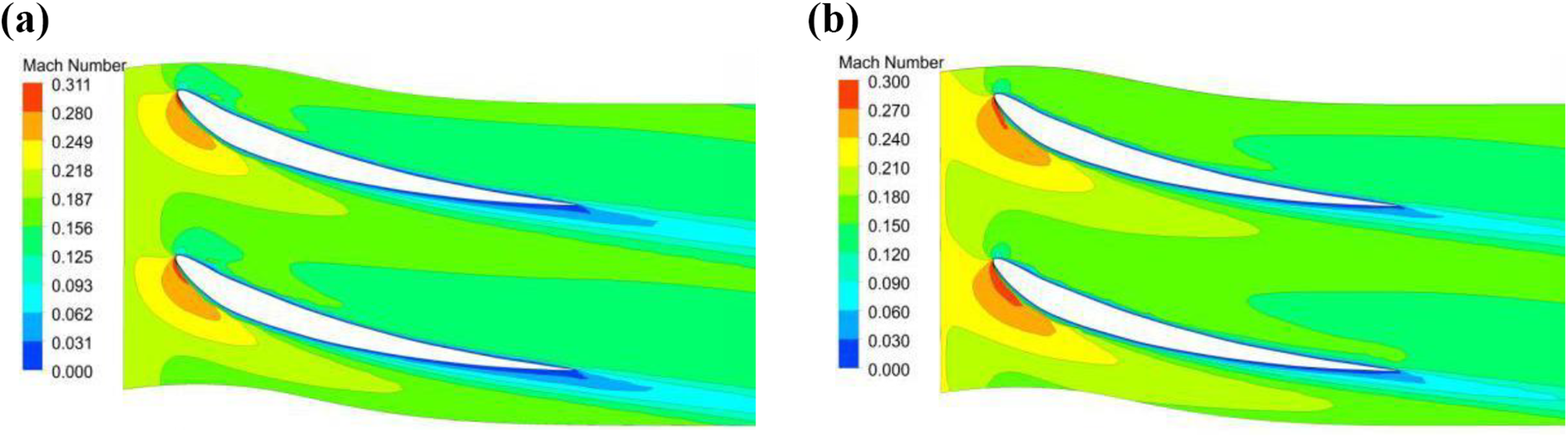
Figure 3(a) and (b) shows the Mach number distribution of the cascaded channel at lower flow rates for the smooth surface of the blade and the blade of the blank surface, respectively, as can be seen from the figure the Mach number distribution of the two. There is a huge difference, and the surface morphology of the blade has a great influence on its flow field.

Figure 3.

(a) Mach number distribution of smooth blade cascade channel. (b) Mach number distribution of cascade channel of blank blade.

Figures 4 to 7 show the Mach number distribution of the cascade channel in the case of roughness in the above table. It can be seen from the figure that as the roughness of the blade surface becomes smaller and smaller, the wake is more and more narrow, and the performance of the blade is gradually improved. When the surface roughness K_s is 4.96, the flow field Mach and the smooth blade are almost the same.

Figure 4.

(a) Distribution of cascade Mach number at K _s = 316. (b) Distribution of cascade Mach number at K _s = 78.

Figure 5.

(a) Distribution of cascade Mach number at K _s = 19.5. (b) Distribution of cascade Mach number at K _s = 9.9.

Figure 6.

(a) Distribution of cascade Mach number at K _s = 4.9. (b) Distribution of cascade Mach number at K _s = 2.5.

Figure 7.

(a) Distribution of cascade Mach number at K _s = 1.2. (b) Distribution of cascade Mach number at K _s = 0.62.

Engine blade performance can be evaluated using two basic indicators, the total pressure loss coefficient and the surface static pressure coefficient, and the expressions are

C P_{T} = \frac{P_{1}^{*} - P_{2}^{*}}{P_{1}^{*} - P_{1}}

C P_{S} = \frac{P - P_{1}}{P_{1}^{*} - P_{1}}

In the above two formulas, $P_{1}^{*}$ and $P_{2}^{*}$ , respectively, represent the inlet total pressure and the outlet total pressure of the blade cascade passage, $P_{1}^{}$ is the inlet static pressure, and P is the static pressure of the blade surface measurement point in the airflow. The relationship between total pressure and static pressure is as follows

\frac{P^{*}}{P} = (1 + \frac{k - 1}{2} {Ma}^{2}) exp (\frac{1}{k - 1})

Among them, Ma is the Mach number of the airflow, and its value is 1.4.

The numerical simulation results are analyzed, and the total pressure loss coefficient and the surface static pressure coefficient of the observation points on the pressure surface and the suction surface of the blade are, respectively, investigated. These observation points are respectively located at equidistant positions along the axial direction, as shown in Figure 8.

Figure 8.

Distribution of static pressure coefficient observation point.

Figure 9(a) is the regular curve of the total pressure loss coefficient of the cascade with the K_s of the equivalent gravel. As the surface roughness of the blade increases, the total pressure loss coefficient of the cascade generally increases. When K_s is greater than 9.9, the upward trend is very obvious, the increase of this loss cannot be ignored, and the surface roughness of the blade must be reduced to reduce the total pressure loss coefficient. However, when the value of K_s is in the (0.62, 3.48) interval, the total pressure loss coefficient is slightly lower than that of the smooth blade.

Figure 9.

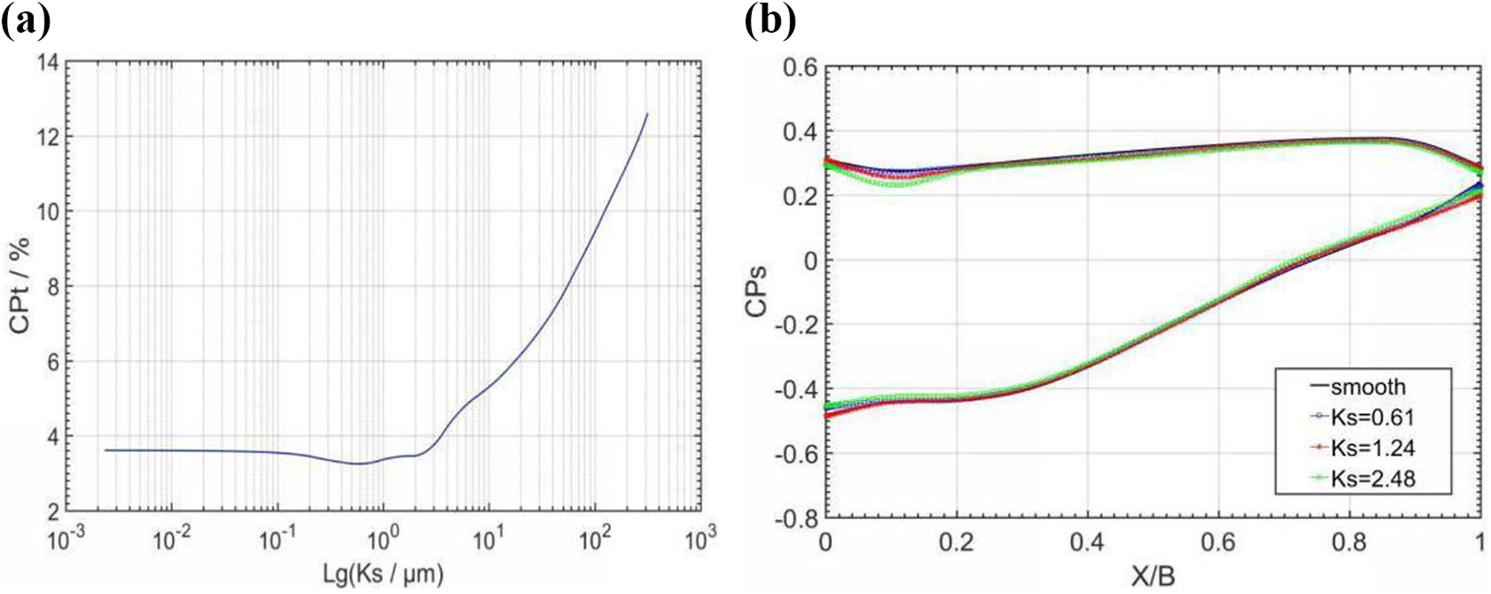
(a) The total pressure loss coefficient changes with K _s. (b) The blade static pressure coefficient curve changes with K _s (0.61, 1.24, 2.48).

Figure 9(a) and (b) shows the blade static pressure curve when the surface roughness is from the blank state to the smooth state. When the blade surface is smooth and nearly smooth, and K_s is 0.61, 1.24, and 2.48, as shown in Figure 9(b), the static pressure coefficient curves almost overlap, showing that the load forces of the blades are almost equal. As shown in Figure 10(a), when the values of K_s are 4.96, 9.98, and 19.9, the static pressure coefficient curve of the blade pressure surface is shifted downward in the y-axis direction, and the static pressure coefficient curve of the suction surface of the blade is shifted upward in the y-axis, corresponding to each roughness. The area enclosed by the pressure surface and the suction surface curve gradually decreases with the increase of the roughness, and the load capacity of the blade decreases as the surface roughness increases. As shown in Figure 10(b), this trend is even more pronounced when K_s continues to rise, and the performance of the blade blank without surface processing is less than half that of smooth blade performance.

Figure 10.

(a) The blade static pressure coefficient curve changes with K_s (4.96, 9.98, 19.9). (b) The blade static pressure coefficient curve changes with K_s (78,316 unpolished).

Robot-based blade machining

The advantage of the robot’s technology for machining the surface of the blade is not only the control method of the fitting and path of the blade surface but also the significant improvement of the formation and adjustment of the production line.^9,23

–26 The cooperation of the robot and the blade positioner, or the robot group, can solve many spatial problems. Previous research has often been carried out on the arrangement of one way. Even if it is improved, it is difficult to adapt to the blade processing of various sizes and various geometries.^27,28 The reason is that the research is costly and the research time is too long. Therefore, reports on such studies are rare. Although the various methods are costly and time-consuming, the research team of this article has carried out research on the layout of several robots, positioners, and robot groups.

Robot holding small belt machine

Small grinding tools can be clamped on the robot’s actuator end. Commonly used are small belt machines, various types of grinding wheel heads for grinding blades, and pneumatic grinding wheels for advanced polishing. The research of the belt sander for the surface polishing of the blade is relatively common, but the difficulty of this method lies in the control of the contact force between the contact wheel of the belt machine and the surface of the blade.

Figure 11(a) is a physical diagram of the abovementioned robot clamping small tool and a typical blade, wherein Figure 11(b) is the connection diagram between the robot execution end and the belt machine. The researchers in this article believe that this type of robotic arrangement is suitable for blade surface machining in the following cases.

Figure 11.

(a) Robot clamping small grinding tool. (b) The blade of the back basin is relatively flat and the air inlet and exhaust sides are straight.

First, the volume of the blade is relatively small, generally the blades of the high-pressure compressor (e.g. stages 4, 5, and 6) and the blades of the low-pressure turbine (e.g. the first, second, and third stages).

Second, the stacking shaft is a straight-lined blade that is easily clamped to the positioner shown in the drawings. Generally, the blade positioner has two degrees of freedom about the z-axis and y-axis. If the stacking axis of the blade is a curve, or a combination of a curve and a straight line (e.g. a curved blade), the use of this form of machining will make the calculations a large number, the established model is too complicated, and is limited by the change. The degree of freedom of the positioner is difficult to adjust the spatial position of the blade, and it is highly probable that the robot will interfere with the surface of the blade, which is disadvantageous for processing.

Third, the geometry is relatively regular, and there are no blades that are designed to have a large spatially distorted shape. In fact, the fan blades of the large bypass ratio turbofan engine and the compressor blades of the low-pressure machine have a certain degree of distortion, but the shapes of the high-pressure compressor and the turbine blades tend to be flat and regular. The blade shown in Figure 11(b) has generally shaped and blade back, with the inlet and exhaust edges tending to be straight, or tending to a regular curve.

Fourth, the blade processing time is not particularly long, and the feed rate during processing is relatively fast. Due to the limitation of the life of the non-starting belt, the total length of the belt of the small belt machine that can be added is relatively short. If a large area is processed for a long time, the abrasive grains adhering to the belt will wear and lose processing. Function, therefore, the entire surface of the blade can be processed within the life span of a single abrasive belt, and the material removal amount of the blade surface cannot be too large, and rapid automated finishing will be the main application object of this form of robot processing.

Robot holding blade

Within the range of the robot’s holding force, it is possible to hold not only the tool but also the workpiece to be machined. The robot’s actuator grips the blade in a form that allows the blade to be machined with greater freedom of machining, allowing for more complex displacements in space. Some of the more complex surfaces, such as compressor low-pressure grade blades with a certain degree of distortion, because each of their stacking surface contours is complex curves, the two-degree-of-freedom positioner described above cannot make them. It has a full spatial displacement, or some small aspect is wider than the blade of the blade. Many displacement mechanisms do not have enough accommodation space to hold the blade and totally complete the change of degrees of freedom. The position is expressed by the interference between the blade being machined and the positioner itself, which makes the machining impossible.

Figure 12 shows the experimental physical map of this form.

Figure 12.

(a) Robot clamping blade and (b) horizontal belt machine as grinding tools.

The robot holds a blade with torsional shape characteristics. The grinding tool uses a horizontal belt machine. The contact wheel of the belt machine has no other spatial motions but only rotation. The path of the blade surface shape is fitted by the spatial motion of the blade itself. The research in this article believes that this form of robotic arrangement can be applied to the following blade processing situations.

First, the blade has a certain shape of torsion or bending. The blade of this shape is generally the first- and second-stage compressor blade of the turbojet engine and the last two stages of the turbine blade.

Second, the compressor blades have a chord width exceeding a certain size. These blades contain both small chord-shaped blades with wide chords and wide-chord blades with equal-chord ratios. Even the projection shapes of some blades tend to be square. The typical shape of such a blade is shown in Figure 13(a).

Figure 13.

(a) Blades with a twisted shape and a square projection. (b) The blade with curved inlet and exhaust sides.

Third, some blades have no conventional basins and leaf backs, and the intake and exhaust sides are not straight lines or curves with lower curvature values, but several curves with larger curvatures are connected. The vanes shown in Figures 13(b) are having a narrower intake and exhaust sides, a very large radius of curvature, and a sharper edge. The intake and exhaust sides are not only straight lines but also have a wavy shape and a large undulation.

Fourth, the processing time of the blade can be extended appropriately, which is suitable for rough machining with large removal of the surface of the blade, and for finishing with consistency requirements on the surface of the blade.

Since the belt machine is set to be fixed, the spatial relationship between the blade and the grinding tool tends to be simple, and the amount of data that the robot system needs to process is greatly reduced.

Robots group

Robot group means there are more than two robots at the same time, which can form a blade surface grinding system based on robot group. Each robot has its own work task. We adopt a combination of such a form; the robot arm holds the blade and makes the blade do the space action which is used to expose different areas of the blade to the active area of the grinding tool. The robot B holds the grinding tool, and the grinding tool fits the surface of the blade and removes the material of the blade surface and the residual milling texture. Figure 14 shows a combination of two robots.

Figure 14.

Robot combination consisting of two robots.

Due to the use of multiple robots, both the machined blade and the grinding tool have a high range of motion. The blade that is being bucked can not only adjust the position to reveal different processing areas but also adjust the posture to adapt to the curvature and direction of the grinding tool in the same processing area. In the research of this article, the grinding tool adopts a polishing head with a very long life, and the polishing head has various specifications of the diameter of the abrasive particles and the number of meshes. The clamping device has the design features of rapid positioning and replacement, so as to improve the accuracy of grinding while reducing the number of calibrations. The author believes that such a robot group is suitable for blade processing of the following characteristics.

First, a compressor blade having a large torsional shape, such as a fan of a large bypass ratio turbofan engine and its first- and second-stage compressor blade. When processing these blades, in order to always have the blade surface and the grinding tool have good contact force and correct contact area during processing, the spatial orientation of the blade and the various inclination angles of the grinding tool are often adjusted at any time.

Second, the high-pressure ratio blade with the damper table. In the engine operation, the pressure surface and the suction surface of the high-pressure ratio of the low-pressure compressor stage are subjected to tremendous pressure and suction at the same time. To maintain the stability of the blade and ensure the interference of the cascade gap without force, such blades are often designed. In the form of a damper, as shown in Figure 15(b), the application of robotics groups has made it easy to solve complex motion trajectory planning.

Figure 15.

(a) Static blade with large twist. (b) High-pressure ratio blade with damper table.

Third, turbine blades and hollow turbine blades with cooling film holes. In the processing of such blades, in order not to damage the film pore structure of the surface, the trajectory planning of the grinding tool is often complicated, and if grinding is performed using a grinder-type tool, processing is difficult.

Large robot and belt machines group

Large-sized blades and heavy-weight blades are difficult to clamp effectively for small- and medium-sized robots. It is prone to interference caused by insufficient operation space of the robot arm during clamping work, or jitter and deformation caused by insufficient bearing quality of the robot. Using a large, high-load robot for clamping, the gripping end of the manipulator has a high enough height, the radius of gyration of the manipulator is long enough, and large blades can easily achieve space action without having to consider interference too much. The robot has a large enough load capacity to hold large-quality blades, especially high-pressure turbine blades, tail nozzle blades, and combustion chamber spoiler blades with high-density high-temperature nickel-based alloy materials. The stiffness avoids the jitter in the adjustment of the blade space and the blade pose error caused by the jitter and can effectively avoid the resonance and vibration when the highly rotating grinding tool feeding on the blade surface.

Figure 16 shows the large robot and belt assembly of the researcher. As shown in Figure 16, four belt machines are distributed around the robot in a C-shaped shape, and their respective tasks are formulated in a counterclockwise direction. They are prepared respectively for roughing, semi-finishing, finishing, and surface polishing. For different shape blades, the curvature of the contact wheel can be matched to the contour curve of the blade by replacing the contact wheel. This form of arrangement can process almost all of the engine’s large blades, including guided turbine blades with two-way boring. Figure 17 shows a stage-oriented turbine blade having a length of about 45 cm and a mass of 7.638 kg. It can be seen that large robots have great advantages for nickel-based alloy materials with high-density processing materials (such as Incoloy 901 and Inconel 718). Nickel-based superalloys are not only widely used in turbines but also used in some advanced engines compressor blades at high temperatures, because the creep limit of titanium alloys is drastically reduced in environments exceeding 400°C, the compressor blades of high performance engines are operating at higher temperatures, and nickel-based alloys are used instead of titanium alloys. This part of the blade is necessary. This change makes the blade being machined difficulty.

Figure 16.

Large robot and belt machines group.

Figure 17.

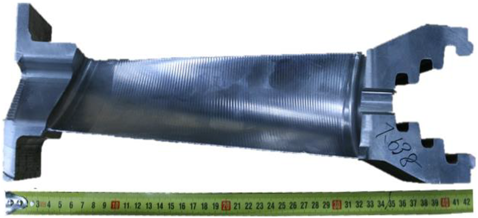
Heavy-duty stationary blades.

Due to the large mass of the blade held by the actuator end, its gripping tool is correspondingly increased, so that it has a large clamping force to prevent the blade from falling and slipping. The opening and closing tension of the clamping tool depends on the tail of the blade. For larger volume blades, the clamping process must have a sufficient opening and closing tension to ensure that the holding tool does not interact with other parts during the opening and closing process. In the event of interference or collision, the corresponding protective measures must be added. Figure 18(b) shows the gripper cover of the robot actuator end, which effectively blocks the various interference from signal wires and power cord attached to the robot arm during processing.

Figure 18.

(a) Belt machine with two degrees of freedom. (b) Clamping guard with warning color.

Experiment

Figure 19 is a schematic diagram of the relationship between the main components of the experimental system. Different from other commonly used methods such as pneumatic grinding wheel, chemical mechanical grinding, and so on,^8,29 in this system, the main control computer is the core component, the robot is the actuator, the rotating platform and the blade positioner are the auxiliary parts, and the grinding tool is fitted. The path planning method of the blade surface has been discussed in detail in the previous chapter. The force sensor and the data acquisition system form a contact force control system to ensure the uniformity of the force on the surface of the blade.

Figure 19.

Experimental system framework.

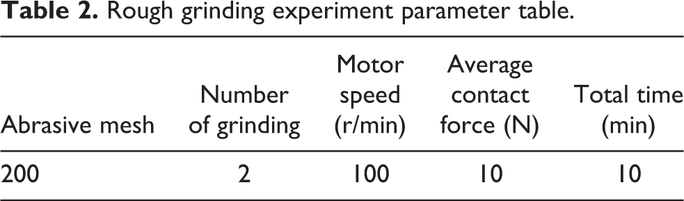
The experimental parameters are listed in Tables 2 and 3. Figures 20 and 21 show the experimentally obtained blade surface. To visually distinguish the experimental results, the upper half of the blade near the tip of the blade was tested, and the lower half of the blade root remained intact. Surface texture, after several times of grinding, the back surface of the blade in Figure 20, has been shown to be close to the mirror surface. After measurement, R _a is less than 0.8, which meets the surface roughness requirements of the blade discussed in chapter 1. Figure 21 shows the grinding results of the blade basin surface. When the grinding times and the shape of the grinding tool are the same, the grinding result of the blade surface will lag behind the blade back surface.

Table 2.

Rough grinding experiment parameter table.

Abrasive mesh	Number of grinding	Motor speed (r/min)	Average contact force (N)	Total time (min)
200	2	100	10	10

Table 3.

Fine grinding experiment parameter table.

Abrasive mesh	Number of grinding	Motor speed (r/min)	Average contact force (N)	Total time (min)
800	2	100	10	10

Figure 20.

Blade back surface after grinding.

Figure 21.

Blade basin surface after grinding.

The processed blade surface must be carefully measured to determine whether the blade has a single factor or multi-factor machining error as described in chapter 1, and the investigator selected an area, as shown in Figure 22. This area has a square tool setting table, and these points are measured and the measured values of these measuring points are compared to the blade design values.

Figure 22.

Distribution of detection points in the grinding area.

Table 4 lists several values selected from these measurement points, zd is the design value in the z-direction, and zm is the measurement value in the z-direction. It is not difficult to find that the surface topography error is controlled in the design within the allowable error range.

Table 4.

Display of measured and design values from selected points on the blade surface.

Point name	x (mm)	y (mm)	zd (mm)	zm (mm)	z Error
P11	11.000	10.000	15.17657	15.175	≤ 0.02
P14	35.000	10.000	18.12891	18.127	≤ 0.02
P22	19.000	18.000	16.37563	16.362	≤ 0.02
P33	27.000	26.000	17.00836	16.982	≤ 0.02
P41	11.000	34.000	15.11843	15.104	≤ 0.02
P65	51.000	50.000	15.80894	15.781	≤ 0.02
P73	27.000	58.000	15.48347	15.475	≤ 0.02

To visually demonstrate the precision that can be achieved by this method, the researcher draws the design values and measured values of the selected points into a three-dimensional picture. Figure 23(a) shows the design of the selected measurement area of the blade. Figure 23(b) is the three-dimensional surface drawn by the measurement points in the above area. From the data analysis, each detection point is within the error control range, and the surface after the blade processing is qualified; visually, there is no significant difference between the processed surfaces and the surface of the design is very close to the design surface. It is reasonable to use a force sensor to implement a force control strategy for the processing of small blades.

Figure 23.

(a) Design surface of the blade. (b) Machined surface of the blade.

This article focuses on the surface micro-morphology of the blade. Figure 24 shows a macroscopic view of the surface of the blade before processing and its micrograph. This image is used to compare the surface topography after processing. Obviously, there is a significant milled texture on the unmachined surface. In the 200-fold magnification of the micrograph, the milled texture has a distinct mountain-shaped ridge line with small traces of the knife. These small traces are perpendicular to this ridge line.

Figure 24.

Microscopic map of the surface of the blade before processing by magnifing 200 times.

Figure 25 shows the local macroscopic effect of the blade after surface processing. Different from the blade tip position selected in the above to measure the surface shape error, at this time, we selected the blade root position as the observation object. The three positions A, B, and C on the blade surface were selected as measurement points, and their surface topography micrographs were taken.

Figure 25.

Partial surface macroscopic view of the blade after processing.

Figure 26 shows an enlarged view of the surface topography of the three observation points described above. Figure 26(a) shows the surface micro-morphology of the processing missing area because the contact wheel did not touch the blade surface. Figure 26(b) shows the surface microtopography of the highest point of the blade back. Figure 26(c) shows the surface microtopography of the area near the exhaust edge.

Figure 26.

(a) Surface topography micrograph of region A. (b) Surface topography micrograph of region B. (c) Surface topography micrograph of region C.

By measurement and comparison, the surface accuracy of the B region is the highest, which reaches R _a = 0.4. The surface roughness of all processed areas is less than 0.8, meeting the requirements for ensuring the basic performance of the blade.

Conclusion and outlook

In this article, the influence of blade surface quality and machining shape error on blade performance was studied. The significance of the blade surface roughness on its performance was to determine the degree of surface quality required for blade surface processing, with original roughness or original milled texture would have a negative impact on its performance, but the machining accuracy was too high, causing problems such as too long a production cycle and huge processing costs. Through numerical calculations, it could be found that when the surface quality reaches a certain level, the surface quality of the blade was continuously improved, and the guarantee effect on its performance would be weakened. Under this circumstance, continuing to improve the surface quality of the blade had no positive effect on the performance of the blade, resulting in waste of manufacturing costs.

Studies had shown that when the blade surface equivalent grit roughness K_s reaches 4.96 (about R_a = 0.8 µm), the blade performance was close to the smooth surface of the blade, and no further processing was required to improve the surface roughness. When the surface equivalent grit K_s was greater than 4.96 µm, the surface roughness had a great influence on the blade performance. When K_s was larger than 40 µm, the negative effect was significantly increased.

This article pointed out that the robot can not only clamp the grinding tool but also the blade workpiece. For the different characteristics of the blade and different processing conditions, four kinds of robot-based blade surface grinding schemes were proposed, of which the core content was the robot layout. Based on the robot group’s fitting to the spatial surface and the path planning, the experimental verification was carried out.

It could be seen from the experiments in this article that after twice surface grinding, the surface roughness of the blade had reached less than 0.8, and this surface precision could ensure the design performance requirements of the blade.

Footnotes

Declaration of conflicting interests

The author(s) declared no potential conflicts of interest with respect to the research, authorship, and/or publication of this article.

Funding

The author(s) received no financial support for the research, authorship, and/or publication of this article.

ORCID iD

Lei Qiu

Liangtao Qi

References

Zettner

Yoda

. Particle velocity field measurements in a near-wall flow using evanescent wave illumination. Exp Fluids 2003; 34(1): 115–121.

Yeom

Park

, et al. Simulation of microstructures for alloy 718 blade forging using 3D FEM simulator. J Wuhan Univ Hydraulic Elect Eng 2000; 141(3): 337–342.

Zhan

Yuli

. Research on a new remeshing method for the 3D FEM simulation of blade forging. J Mater Process Tech 1999; 94(2-3): 231–234.

Koca Da

Czy Ewski

Mehdi

. Numerical analysis of lateral forces in a die for turbine blade forging. Arch Civ Mech Eng 2009; 9(4): 49–54.

Zhan

Yang

Liu

. Deformation characteristic of the precision forging of a blade with a damper platform using 3D FEM analysis. J Mater Process Tech 2004; 150(3): 290–299.

Shan

Zhang

, et al. Precision forging process analysis and preform optimization of small compressor blade of titanium alloy. Appl Mech Mater 2013; 364: 493–499.

Cheng

Wei

. Optimization on precision forging process of double-mounting plates stator blade of titanium alloy. Mater Sci Technol 2013; 21(4): 131–137.

Zeng

S M

Jin

M S

, et al. Investigation on machining characteristic of pneumatic wheel based on softness consolidation abrasives. Int J Precis Eng Man 2014; 15(10): 2031–2039.

Zeng

Jin

, et al. Research on dynamic characteristic of softness consolidation abrasives in machining process. Int J Adv Manuf Tech 2016; 82(5-8): 1115–1125.

10.

Márquez

Pérez

Rios

, et al. Process modeling for robotic polishing. J Mater Process Tech 2005; 159(1): 69–82.

11.

Liao

Liu

. Modeling and control of automated polishing/deburring process using a dual-purpose compliant toolhead. Int J Mach Tool Manu 2008; 48(12-13): 1454–1463.

12.

Lai

Zhang

, et al. Digital manufacture of large-grade hydro turbines blades. J Mater Process Tech 2009; 209(11): 4963–4969.

13.

Yan-Zong

. Experimental study on roughness of sand-concrete structure interface. Build Sci 2013; (1): 13.

14.

Vulchanov

Zimparov

. Stabilized turbulent fluid friction and heat transfer in circular tubes with internal sand type roughness at moderate Prandtl numbers. Int J Heat Mass Tran 1989; 32(1): 29–34.

15.

Qiu

Zeng

, et al. Research on combustion chamber structure improvement and ignition system of missile turbojet engine for diesel fuel. Teh Vejsn 2018; 25(6): 1792–1800.

16.

Hou

Christensen

. Influence of equivalent sand roughness on the dispersion coefficient in laboratory and natural streams [Pollutant transport problems]. In: 3. Symposium on Inland Waterways for Navigation, Flood Control, and Water Diversions, Ft. Collins, CO, USA, 10–12 August 1976.

17.

Morini

Pinelli

Spina

, et al. Numerical analysis of the effects of nonuniform surface roughness on compressor stage performance. J Eng Gas Turb Power 2011; 133(7): 745–753.

18.

Coleman

. Measurement and prediction of the effects of nonuniform surface roughness on turbulent flow friction coefficients - 1st National Fluid Dynamics Conference (AIAA). J Fluids Eng 1988; 110(4): 380.

19.

Sutherland

. LII. The viscosity of gases and molecular force. Philos Mag 2009; Edinburgh(36): 507–531.

20.

Launder

Spalding

. The numerical computation of turbulent flows. Comput Method Appl M 1974; 3(2): 269–289.

21.

Menter

. Two-equation eddy-viscosity turbulence models for engineering applications. AIAA J 1994; 32(8): 1598–1605.

22.

Koch

Smith

. Loss sources and magnitudes in axial-flow compressors. J Eng Gas Turb Power 1976; 98(3): 411–424.

23.

Qiu

Zeng

, et al. Chemical mechanical polishing of titanium alloy based on transmission electron microscopy. Asta Microscopica 2019; 28(5): 1133–1141.

24.

Sun

Giblin

Kazerounian

. Accurate robotic belt grinding of workpieces with complex geometries using relative calibration techniques. Robot CIM-INT Manuf 2009; 25(1): 204–210.

25.

Ren

Cabaravdic

Zhang

, et al. A local process model for simulation of robotic belt grinding. Int J Mach Tool Manu 2007; 47(6): 962–970.

26.

Burghardt

Kurc

Szybicki

. Robotic automation of the turbo-propeller engine blade grinding process. Appl Mech Mater 2016; 817: 206–213.

27.

Gang

, et al. 3-D Shape matching of a blade surface in robotic grinding applications[J]. IEEE/ASME Trans Mech 2016; 21(5): 2294–2306.

28.

Sabourin

Paquet

Hazel

, et al. Robotic approach to improve turbine surface finish. In: Hazel

(Ed) 2010 1st international conference on applied robotics for the power industry, Delta Centre-Ville Hotel, Montreal, Canada, 5 October, 2010, pp. 1–6. IEEE.

29.

Huang

Cheng

, et al. Kinematics analysis of abrasive belt grinding robot for aero-engine blade and its simulation. Adv Mater Res 2014; 889-890: 1165–1169.

The blade surface performance and its robotic machining

Abstract

Keywords

Introduction

Blade surface roughness model

Wall function correction

Governing equation of near-wall airflow

Machining accuracy and performance of blade surface

Model of blade cross section

Analysis results

Robot-based blade machining

Robot holding small belt machine

Robot holding blade

Robots group

Large robot and belt machines group

Experiment

Conclusion and outlook

Footnotes

Declaration of conflicting interests

Funding

ORCID iD

References