Continuous reinforcement learning to adapt multi-objective optimization online for robot motion

Abstract

This article introduces a continuous reinforcement learning framework to enable online adaptation of multi-objective optimization functions for guiding a mobile robot to move in changing dynamic environments. The robot with this framework can continuously learn from multiple or changing environments where it encounters different numbers of obstacles moving in unknown ways at different times. Using both planned trajectories from a real-time motion planner and already executed trajectories as feedback observations, our reinforcement learning agent enables the robot to adapt motion behaviors to environmental changes. The agent contains a Q network connected to a long short-term memory network. The proposed framework is tested in both simulations and real robot experiments over various, dynamically varied task environments. The results show the efficacy of online continuous reinforcement learning for quick adaption to different, unknown, and dynamic environments.

Introduction

Real-time motion planning of robots often needs to consider multiple and sometimes conflicting optimization criteria, such as time efficiency (in terms of the shortest distance or time), safety (in terms of the clearance to obstacles), and energy efficiency. ^{1 –3} A common practice is to combine these criteria in a cost function as a weighted sum. However, determining proper values for the coefficients in the cost function is not a trivial issue but often done manually in an ad hoc manner. It is difficult to determine the coefficient values of a combined optimization function before having the robot perform in an environment (i.e. all the set values may not be optimal). Moreover, when the task environment changes, the previously set coefficient values may not be suitable anymore.

Hence, there are two related open problems: (1) how to determine values for coefficients of a compound optimization function automatically and (2) how to make the coefficients self-adapt to environmental changes. There is little work on both problems. Ishigami et al. ⁴ tried to generate different paths with different sets of coefficients and evaluate theses paths based on a metric, but the values of all coefficients still need to be set off-line manually. The main contribution of this article is that we propose to tackle both problems by continuously training a reinforcement learning (RL) agent in different environments, even during the test. The agent is trained to adjust the values of the coefficients of a multi-objective optimization function based on the robot’s performance in an environment with unknown dynamic obstacles, and the agent keeps learning by itself to best adapt to all kinds of environmental changes continuously. During the process, the agent becomes more and more knowledgeable and better and better at learning.

Specifically, we introduce a continuous RL agent that leverages motion planning results and can accommodate real-time robot motion planning methods. The observations of the agent are motion trajectories, whose dimension is far lower than the dimension of raw sensor data (such as the image of a camera) that is often used in end-to-end learning. Therefore, a convolutional neural network (NN) that is used to extract observation features can be removed from the agent. This simplifies the formulation of the agent and enables continuous learning. Learning continuously means that ^{5 –7} the agent can accumulate the knowledge learned in the past environments to help future learning and problem-solving and that later learning does not degrade much its performance in task environments learned earlier.

Related work

Lifelong or continuous learning has been a long-standing challenge for machine learning and autonomous systems. ^{8 –10} Mimicking humans and animals that continuously acquire new knowledge and transfer them to new tasks throughout their lifetime, continuous learning builds an adaptive system that is capable of learning from a continuous stream of information. However, dilemma between plasticity and catastrophic forgetting ^11,12 is the main challenge due to inefficiency and poor performances when relearning from scratch for new tasks. ⁶ Thus, accommodation of new knowledge while not forgetting or interfering current learning process requires a sophisticated approach to consolidate knowledge. Memorizing past experiences ^{13 –15} or allocating NN resources dynamically ^16,17 has been introduced to alleviate the forgetting problems. Replaying previous experiences ^18,19 improves learning efficiency by reducing sequential dependence of data and forgetfulness of important experiences, but experience replay only does not provide enough self-adaptability to dynamically changing environments.

Acknowledging the impossibility of providing all the prior knowledge to perform well in the real-world, continuous learning models has been emerged for robots. One aim of the continuous learning is to train an agent that can quickly adapt to new tasks (e.g. changing navigation goals or environments). A hierarchical Bayesian model ²⁰ has been used to transfer the knowledge learned between different but related tasks. Actor-Mimic ²¹ conducts the training over related source tasks, but the generalization to new target tasks needs a sufficient level of similarity between the source and the target tasks. Zhang et al. ²² employ the conception of successor factors into RL. Besides, universal value function approximators (UVFAs) ²³ propose to handle different goals in one environment by incorporating the goal into the input of the value function. The generalization ability of navigating new tasks can also be achieved by combining RL with conventional motion planning methods. ^24,25 However, the above method can only transfer the learned knowledge to new tasks just slightly changed from the training tasks, for example, removing or adding one or two static obstacle(s) in the test environment.

A few researchers consider transferring the trained agent to totally different environments with only static or moving obstacles. For example, one method called reinforcement planning ²⁶ extends RL to automatically learn cost functions for search-based planners such as A* and Dijkstra’s algorithm. The method successfully transfers the trained agent to some new static environments without moving obstacles, but it lacks the ability to improve the performance continuously as the learning progresses in different, dynamically changing environments. Everett et al. ²⁷ use a long short-term memory (LSTM) network to handle an arbitrary number of obstacles, but there are only moving obstacles and the number of moving obstacles is fixed in each environment. There is little research on solutions that can continuously train an RL agent with feedback to adapt the robot motion to changing mixed environments, where there are a variable number of static and moving obstacles. This leads us to propose a continuous, incremental knowledge acquisition model, which is essential for a lifelong learning robot that does not lose important knowledge obtained through a motion planner.

Overview of the framework

The proposed framework is illustrated in Figure 1. There are two closed loops: one is among a real-time motion planner, a robot, and an environment and the other one is between the real-time motion planner and an RL agent. In the first closed loop, the real-time motion planner interacts with the task environment based on sensing and generates the best motion trajectory according to the current multi-objective cost function for the robot to execute. Here, the “coefficients” are used in the linear combination in the cost function. In the second closed loop, an RL agent develops proper coefficients for the multi-objective cost function to maximize the desired performance in real-time motion planning.

Figure 1.

Continuous RL with motion planning. RL: reinforcement learning.

The RL agent has three NNs: an LSTM NN, an online NN, ²⁸ and a target NN. The three networks can be classified in two parts. One includes the LSTM network, which is used to preprocess the motion trajectories. This will be described in detail in “Observation” section. The other includes the online network and the target network, which are used for RL. The online network is continuously trained based on the continuous observation, reward, and loss calculated using the target value from the target network. The target network is created by copying the online network during initialization. During training, only the online network is trained, and then its weights are copied to the target network periodically. Note that directly implementing RL with only the online network is unstable, because the network being trained is also used to calculate the target value. To solve this problem, the separate target network is used to calculate the target value. The target network can greatly improve the stability of continuous RL and enable the agent to continuously build skills on how to adjust the coefficients to best adapt to environmental changes. If we use only the online network, the learning is prone to diverge. Note that the NN weights in RL and the planner’s optimization function coefficients are different. The former is trained through backward propagation, and the latter is tuned by the RL agent.

The proposed framework is validated by a case study with the real-time adaptive motion planner (RAMP) ^29,30 and can be easily extended to benefit other real-time motion planners. The framework has the following characteristics:

The skills learned from the earlier task environments are accumulated and used to make the learning in the current task environment more efficient.

While the robot benefits from the learned skills provided by the learning agent to perform and adapt well in constantly changing environments, the learning agent itself is trained continuously through the online network to improve its own performance.

The proposed framework is general and abstract and, hence, is independent of real-time motion planners, platforms, and task environments.

The agent does not learn specific coefficients but learns a mapping from motion trajectories to coefficient changes. This enables the robot to adapt to different numbers of obstacles moving in unknown ways during the navigation.

The learned skills can be transferred to different types of task environments and motion planning objectives and from a simulated world to the real world.

By using motion trajectories as feedback observations, the formulation of the RL agent is greatly simplified. This makes continuous training much more efficient and hence effective.

The learned optimization coefficients have clear meanings, so the resulting robot performance is understandable. This feature allows us to analyze the relationship between robot motions and coefficient changes.

The rest of this article is organized as follows. The fourth section describes our RL strategy. The fifth section provides a case study with RAMP as the motion planner. The sixth section provides and discusses the training and test results in both simulations and real robot experiments. The last section concludes the article.

RL-based coefficient determination

In this section, we will introduce the method of continuously training the RL agent in the proposed framework. Generally, the agent with discrete action space provides better stability than that with continuous action space, so we use Q networks to adjust the coefficients discretely. The input of the Q networks must have fixed length, but the observation input contains a hybrid trajectory with variable length. Therefore, we use an LSTM network to encode the information of the hybrid trajectory into a fixed-length representation.

Besides, when NNs are used in RL, the samples are assumed to be independently and identically distributed. However, when the samples are generated from exploring in an environment sequentially, this assumption doesn’t hold. Therefore, to minimize correlations between samples, the agent is trained off-policy with samples from a replay buffer. Using replay buffer may slow learning, but in practice we found that this is greatly outweighed by the stability of learning.

Observation

An observation is the input of the RL agent, but it does not contain environmental information. First, we are interested in an agent being able to handle different goals, so we follow the approach from UVFA, ²³ that is, the observation includes the navigation goal $\overrightarrow{g}$ . Second, the observation should include the hybrid trajectory that is the real trajectory concatenated with the planned trajectory from a motion planner, because the real trajectory and the planned trajectory capture the information of the robot motion state and the surrounding environment, such as the positions of obstacles. Two examples of hybrid trajectories are shown in Figure 2. The switching of tracked trajectories occurs at the points with numeric marks. In Figure 2(a), the robot is going to follow trajectory 0-B. In Figure 2(b), the robot has arrived at point 1, and the robot’s real trajectory is 0-A′-1, which is different from 0-A-1 due to robot model and motion uncertainty. In Figure 2(c), the robot switches to a new planned trajectory 1-D. In summary, here the hybrid trajectories are 0-A′-1-B and 1-C′-2-D, which are the real trajectories (0-A′-1 and 1-C′-2) concatenated with the unexecuted part (1-B and 2-D) of the planned trajectories.

Figure 2.

Examples of hybrid trajectories: (a) planned trajectory 0-B, (b) hybrid trajectory 0-A′-1-B, (c) switching to planned trajectory 1-D, and (d) hybrid trajectory 1-C′-2-D.

We use $\overrightarrow{g}$ to represent the navigation goal and $\tau (t)$ to represent the hybrid trajectory at a time instant t. A navigation goal is defined as $\overrightarrow{g}=\left(x_g,y_g,{\varphi }_g\right)$ , and a trajectory is a sequence of robot motion states. A robot motion state is a collection of a robot pose, a velocity, and an acceleration with a time stamp. The kth motion state in a trajectory is defined as ${\overrightarrow{s}}_k=\left(x,y,\varphi ,\dot{x},\dot{y},\dot{\varphi },\ddot{x},\ddot{y},\ddot{\varphi },t_k\right)$ , where x and y are the position coordinates, $\varphi$ is the orientation, and t_k is the time stamp of ${\overrightarrow{s}}_k$ . Therefore, we have $\tau (t)=\left({\overrightarrow{s}}_0,{\overrightarrow{s}}_1,\cdots ,{\overrightarrow{s}}_K\right)$ , where K is the number of motion states in $\tau (t)$ .

Note that K is not a constant. Thus, an LSTM NN is used to transfer the variable-length trajectory ( $\tau (t)$ ) into a fixed-length vector ( ${\overrightarrow{h}}_K$ ) that contains relevant information of all motion states, as in handling the varying number of obstacles with LSTM. ²⁷ As shown in Figure 3, the pertinent information of each motion state in $\tau (t)$ is stored in the cell state ${\overrightarrow{c}}_k$ , which is the “memory” of the LSTM network. The cell state acts like a conveyor belt that transfers relative information all the way down the chain. The cell also outputs a hidden state ${\overrightarrow{h}}_k$ based on the current cell state. In mathematical terms, the forward propagation of the LSTM network can be formulated as

Figure 3.

The architecture of the LSTM Q network. LSTM: long short-term memory.

$\begin{array}{ll}{\overrightarrow{f}}_k\hfill & =\sigma \left(W_f\cdot \left[{\overrightarrow{h}}_{k-1}||{\overrightarrow{s}}_k\right]+{\overrightarrow{b}}_f\right)\hfill \\ {\overrightarrow{i}}_k\hfill & =\sigma \left(W_i\cdot \left[{\overrightarrow{h}}_{k-1}||{\overrightarrow{s}}_k\right]+{\overrightarrow{b}}_i\right)\hfill \\ {\overrightarrow{c}}_k\hfill & ={\overrightarrow{f}}_k\circ {\overrightarrow{c}}_{k-1}+{\overrightarrow{i}}_k\circ \text{tanh}\left(W_c\cdot \left[{\overrightarrow{h}}_{k-1}||{\overrightarrow{s}}_k\right]+{\overrightarrow{b}}_c\right)\hfill \\ {\overrightarrow{o}}_k\hfill & =\sigma \left(W_o\cdot \left[{\overrightarrow{h}}_{k-1}||{\overrightarrow{s}}_k\right]+{\overrightarrow{b}}_o\right)\hfill \\ {\overrightarrow{h}}_k\hfill & ={\overrightarrow{o}}_k\circ \text{tanh}\left({\overrightarrow{c}}_k\right)\hfill \end{array}$

1

where $\sigma$ is the sigmoid function, and W_f , W_i , W_c , W_o and ${\overrightarrow{b}}_f$ , ${\overrightarrow{b}}_i$ , ${\overrightarrow{b}}_c$ , ${\overrightarrow{b}}_o$ are the weight matrices and the bias vector parameters. The operators $||$ and $\circ$ denote the concatenation and the Hadamard product.

The LSTM network has the ability to add relevant information of motion states to the cell state. Hence, the final hidden state ${\overrightarrow{h}}_K$ captures the relevant information of all motion states in $\tau (t)$ . The vector ${\overrightarrow{h}}_K$ has a fixed length and is concatenated with $\overrightarrow{g}$ to form a new vector ${\overrightarrow{v}}_g$ , and then ${\overrightarrow{v}}_g$ is fed to a Q network with three fully connected layers. The outputs are the Q values for all possible actions. $\overrightarrow{a}$ is an action vector, which will be introduced in the next section. The learning rate is set to 0.005 initially and reduced to 0.0005 through exponential decay, and other parameters of the LSTM network and the Q network are presented in Table 1.

Table 1.

Parameters of LSTM network and Q network.

Parameter	Value
# Input channels	10
# Hidden layers of LSTM	1
Hidden (output) size of LSTM	20
# Hidden layers of Q network	3
Hidden size of Q network	32
Activation function of hidden layer	ReLU
# Output channels	9
Dropout probability	0.4
# Each batch’s samples	64
# Steps of target network	500

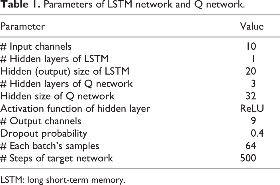
LSTM: long short-term memory.

The best action is selected by the $\epsilon$ -greedy strategy, where $\epsilon$ is the ratio of exploration. At the beginning of learning, we know little about the environment, so we must do more exploration by setting $\epsilon$ to a big value. After the network is trained for some time, we know a lot about the environment, so we can do more exploitation by setting $\epsilon$ to a small value. In a new environment, our $\epsilon$ is set to 0.5 at the beginning of learning and reduced to 0.1 through exponential decay when the network has been trained for 30 episodes in this environment.

Action

Now suppose we have n coefficients W ₁, W ₂, $\cdots$ , W_n that need to be adjusted, which come from the same multi-objective cost function. Note that we are only interested in the relative costs of different candidate trajectories, so coefficient vectors $\left(W_1=1,W_2=1,\cdots ,W_n=1\right)$ and $\left(W_1=2,W_2=2,\cdots ,W_n=2\right)$ are equivalent for the cost function. The degree of freedom (DOF) of coefficient vector $\left(W_1,W_2,\cdots ,W_n\right)$ is only $n-1$ . Therefore, an action is represented as an $n-1$ dimensional vector $\overrightarrow{a}=\left(d_{W_2},d_{W_3},\cdots ,d_{W_n}\right)$ that changes the vector $(W_2,W_3,\cdots ,W_n)$ . Since the action space of the Q network is discrete, the coefficients must be changed discretely at a fixed step d_W ( $d_{W_2},d_{W_3},\cdots ,d_{W_n}\in \{-d_W\mathrm{,0},d_W\}$ ). In other words, each coefficient can be increased or decreased by d_W or remain unchanged at a time. The total number of possible actions is $N_{\text{act}}{=3}^{n-1}$ . If the selected real-time motion planner has multiple optimization criteria whose coefficients need to be adjusted, one of the coefficients can be set to 1.0 and, hence, can reduce one DOF. Other coefficients are adjusted independently.

Reward

An RL agent should learn from performance-driven feedback. This feedback can be modeled as a simple delayed reward function used in the training process, such as the time to reach a goal location or the number of collisions. Our reward r is calculated to evaluate the robot’s performance as follows:

$r=\left\{\begin{array}{cc}{R}_{\text{a}}+\left(T_{\text{m}}-t_{\text{a}}\right)& \text{if at the goal region}\\ -1t_{\text{o}}-I_{\text{c}}\times T_{\text{p}}& \text{if not at the goal region}\end{array}\right.$

2

where

$I_{\text{c}}=\left\{\begin{array}{cc}1& \text{if the robot has collided with obstacles}\\ 0& \text{if the robot has not collided with obstacles}\end{array}\right.$

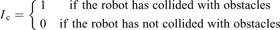
and the constant $T_{\text{m}}$ is the time limit to move from the start location to the goal region. The constant $R_{\text{a}}>0$ is a fixed reward for arriving at the goal region within $T_{\text{m}}$ . The variable $t_{\text{a}}$ is the actual execution time to the goal region. The variable $t_{\text{o}}$ is the estimated time until a collision when moving along the current best trajectory. $t_{\text{o}}$ is $+\infty$ if no collision is predicted. Considering this internally estimated collision time in the reward function can make the robot learn to move at a certain distance from obstacles, because the feedback information about obstacles can be returned before the robot really collides with obstacles. This feature is a superiority of the proposed framework. The constant $T_{\text{p}}$ is the time penalty when a collision occurs in simulation or a forced stop of the robot occurs in real experiments (to avoid actual collisions). By increasing the cumulative reward over time, the robot will try to arrive at the goal region as soon as possible while avoiding collisions. Each training episode will keep going until the robot arrives at the goal region or $T_{\text{m}}$ is reached.

According to equation (2), the agent can only receive a positive reward when it succeeds in arriving at the goal region within the time limit $T_{\text{m}}$ . This feature often reduces the stability and the efficiency of the training. We address this problem by following the approach from Hindsight Experience Replay. ³¹ For the failed navigation, we can double the training samples in replay buffer with disguised successful case, that is, each transition is stored in the replay buffer twice: once with the navigation goal at which the robot failed to arrive within $T_{\text{m}}$ and once with the goal corresponding to the motion state of the robot at time instant $T_{\text{m}}$ .

Updating of weights in NNs

There are totally three NNs in our RL agent: the LSTM network, the online network, and the target network. The weights of the online network and the LSTM network are updated by the backward propagation of the error e, and the weights of the target network are copied from the weights of the online network periodically. The interval (or number of steps) for this copying is a hyper-parameter, which is determined by a pilot test in the simulation. The error e is

$e=y-Q(\overrightarrow{S},\overrightarrow{a})$

3

where

$y=\left\{\begin{array}{cc}r& \text{if at the goal region}\\ r+\gamma \cdot {\text{max}}_{{\overrightarrow{a}}^{\prime }}{Q}^{\prime }({\overrightarrow{S}}^{\prime },{\overrightarrow{a}}^{\prime })& \text{if not at the goal region}\end{array}\right.$

and $\overrightarrow{a}$ is the action vector used to change the coefficients. $\overrightarrow{S}=\left(\tau \left(t\right),\overrightarrow{g}\right)$ is the current observation and ${\overrightarrow{S}}^{\prime }$ is the next observation after applying $\overrightarrow{a}$ . r is the current reward and $\gamma$ is the discounting factor. Note that $Q\left(\overrightarrow{S},\overrightarrow{a}\right)$ is calculated using the online network, and $Q^{\prime }\left({\overrightarrow{S}}^{\prime },{\overrightarrow{a}}^{\prime }\right)$ is calculated using the target network. The backward propagation of e in the online network and the LSTM network are well-known and, hence, are omitted in this article for brevity. ^19,32 The weights of the LSTM network are updated to learn how to transfer a variable-length trajectory into a fixed-length vector. The weights of the target network are updated to learn how to adjust the coefficients of a multi-objective cost function in a real-time motion planner, and the weights of the online network are updated to enable the agent to keep learning from different kinds of environments continuously.

Case study

In this case study, we use the RAMP as a selected motion planner module in the proposed continuous RL framework. We will first review RAMP and then introduce how to utilize it in the proposed framework.

Overview of RAMP

RAMP enables the simultaneous planning and control in dynamic environments. RAMP always maintains multiple trajectories called a population through a trajectory generator. At the start of each control cycle, the lowest cost trajectory in the population is selected as the best trajectory. Trajectory costs are calculated through a trajectory evaluator. While the robot moves along the current best trajectory, RAMP keeps modifying the population based on the latest sensing information. The above process continues until the robot reaches the goal. There are both feasible (collision-free) and infeasible (not collision-free) trajectories in the population. Sometimes the robot has to follow an infeasible trajectory when there is no feasible one, and the robot will stop if a collision will occur within a short time threshold, called imminent collision. While the robot is stopped, RAMP continues to modify the population until (1) it finds a better trajectory for the robot to switch to or (2) the obstacle causing the imminent collision moves away.

RAMP uses different cost functions to evaluate feasible and infeasible trajectories. The cost functions for feasible trajectories and infeasible trajectories are shown in equations (4) and (5), respectively.

$C_{\text{feasible}}=W_{\text{T}}\times \frac{T}{N_{\text{T}}}+W_{\text{A}}*\frac{A}{N_{\text{A}}}+W_{\text{D}}\times \frac{1D}{N_{\text{D}}}$

4

$C_{\text{infeasible}}=W_{T_{\text{c}}}\times \frac{T_{\text{c}}}{N_{T_{\text{c}}}}+W_{A_{\text{c}}}\times \frac{A_{\text{c}}}{N_{A_{\text{c}}}}$

5

where T, A, and D are the estimated execution time, the orientation change, and the distance to the nearest obstacle of the feasible trajectory, respectively, and $T_{\text{c}}$ and $A_{\text{c}}$ are the estimated time until a collision and the orientation change of the infeasible trajectory. They have the corresponding coefficients $W_{\text{T}}$ , $W_{\text{A}}$ , $W_{\text{D}}$ , $W_{T_{\text{c}}}$ , and $W_{A_{\text{c}}}$ and the normalization factors $N_{\text{T}}$ , $N_{\text{A}}$ , $N_{\text{D}}$ , $N_{T_{\text{c}}}$ , and $N_{A_{\text{c}}}$ . Note that the cost for any feasible trajectory is lower than that for any infeasible trajectory. In this case study, $W_{\text{T}}$ is set to 1.0, and $W_{\text{A}}$ and $W_{\text{D}}$ are adjusted by RL. $W_{T_{\text{c}}}$ and $W_{A_{\text{c}}}$ are set to some fixed human-tuned values.

Continuous RL with RAMP

The continuous RL framework after utilizing RAMP is shown in Figure 4. Here, the target NN is hidden for clarity. In Figure 4, the best trajectory generated by RAMP is represented as ${\tau }_{\text{b}}$ . The real trajectory of the mobile robot is represented as ${\tau }_{\text{r}}$ . The hybrid trajectory ( ${\tau }_{\text{b}}$ concatenated with ${\tau }_{\text{r}}$ ) is represented as $\tau$ (the operator $||$ denotes the concatenation). The goal location is represented as $\overrightarrow{g}$ . At the end of each control cycle, the hybrid trajectory is stacked in the replay buffer. Then, the LSTM network takes a hybrid trajectory from the replay buffer through sampling and encodes the motion states of the hybrid trajectory into a fixed-length vector. This vector is concatenated with the goal vector to form a new vector, which is fed to the Q network. At last, the Q network outputs the coefficient changes back to RAMP.

Figure 4.

Case study with RAMP. RAMP: real-time adaptive motion planner.

Results

In this section, we present both the simulation and the real experimental results from the above case study with RAMP.

Simulation experiments

The simulations are conducted on the Gazebo simulator using a four-core i5 2.4 GHz CPU. The Gazebo simulator uses a physical engine. The robot in the simulator needs to receive control commands (linear and angular velocities) and respond to the commands under the constraints of the physical engine, so there are control errors even in simulations. The moving obstacles in the simulations are able to move in different ways. The trajectories of all moving obstacles are unknown to the robot. Only the instant positions and orientations of moving obstacles are sent to the robot as sensed results at a fixed frequency. The size of one simulation environment is 6 $\times$ 6 m². In the other simulation environments, there are working zones bounded by black rectangles and outside walls. The sizes of the working zones are 6 $\times$ 6 m², and the sizes of the outside walls are 8 $\times$ 8 m².

Training

The training environments are shown in Figure 5 (called Tr. A $:$ Tr. D). There are both static obstacles (red barrels) and moving obstacles (blue cars) in the environments. Note that in Tr. D, the static obstacles are dumpsters with black tops, which are bigger than the red barrels. The moving obstacles in Tr. D are also bigger than those in other training environments. All moving obstacles move randomly. Specifically, in every 100 ms, each moving obstacle rotates at a random angular velocity for 20 ms and then advances at a random linear velocity for 80 ms. The ranges of the random angular and linear velocities are approximately 0.3–0.6 rad/s and 1.0–1.4 m/s, respectively. Besides, there are doors that randomly switch or close at different time in Tr. A and Tr. C. In the experiments, we call that the robot completes one episode when it arrives at the goal from the start. The start and the goal of the robot are marked by “1” and “2”, respectively. The working zone of the robot is bounded by a black square. Outside the working zone, there are four walls, by which the motions of moving obstacles are restricted. The robot guided by the motion planner can only run in the working zone, but the moving obstacles can move in or outside the working zone. Therefore, the robot works with different numbers of moving obstacles in one environment at different times. For example, now in Tr. C, there are five moving obstacles in the working zone and three moving obstacles outside the working zone.

Figure 5.

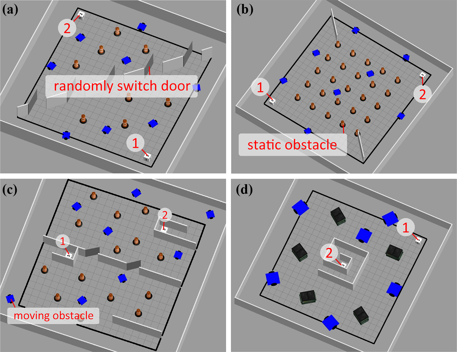
The training environments (note that the blue cars are unpredictable moving obstacles): (a) Tr. A, (b) Tr. B, (c) Tr. C, and (d) Tr. D.

The RL agent was trained for two rounds. In each round, the agent was trained in Tr. A, Tr. B, Tr. C, and Tr. D, sequentially. In each training environment, we trained the agent for 50 episodes and then switched to the next environment. Recall that the coefficients are changed by a fixed step $d_{\text{W}}$ , and the target NN is updated every $T_{\text{u}}$ control cycles. We used different values of $d_{\text{W}}$ and $T_{\text{u}}$ to train the agent, and the results are shown in Tables 2 to 5. According to the results, we obtained the best training performance under the setting of $d_{\text{W}}=0.05$ and $T_{\text{u}}=300$ , so this setting was used in the following simulations.

Table 2.

The average execution time (s) with the standard deviation using different $d_{\text{W}}$ and $T_{\text{u}}$ .

Tu dW	0.03	0.05	0.07	0.09	0.11
50	40.1 ± 1.93	39.8 ± 1.88	41.5 ± 2.87	42.6 ± 3.22	43.3 ± 3.52
150	38.6 ± 1.78	38.2 ± 1.74	39.1 ± 1.89	40.3 ± 2.34	41.1 ± 2.95
300	37.1 ± 1.44	36.7 ± 1.37	37.3 ± 1.56	38.5 ± 1.85	39.9 ± 1.97
450	37.9 ± 1.53	37.5 ± 1.49	38.3 ± 1.75	39.1 ± 1.91	40.7 ± 2.26
550	39.2 ± 1.81	38.3 ± 1.75	40.6 ± 1.99	41.5 ± 2.62	42.3 ± 3.36

Boldface values are used to highlight the maximal or minimal values in the corresponding table.

Table 3.

The average # collisions with the standard deviation using different d_W and T_u .

Tu dW	0.03	0.05	0.07	0.09	0.11
50	3.36 ± 1.02	3.24 ± 0.96	3.57 ± 1.17	3.72 ± 1.31	3.96 ± 1.41
150	2.22 ± 0.78	2.16 ± 0.75	2.36 ± 0.89	2.54 ± 0.92	2.82 ± 1.05
300	1.54 ± 0.47	1.02 ± 0.31	1.71 ± 0.53	1.93 ± 0.69	2.48 ± 0.96
450	1.95 ± 0.68	1.78 ± 0.56	2.24 ± 0.81	2.46 ± 0.84	2.67 ± 0.95
550	2.86 ± 0.93	2.32 ± 0.87	3.06 ± 0.88	3.38 ± 1.07	3.52 ± 1.12

Boldface values are used to highlight the maximal or minimal values in the corresponding table.

Table 4.

The 95% confidence interval of execution time (s) using different d_W and T_u .

Tu dW	0.03	0.05	0.07	0.09	0.11
50	[39.91, 40.29]	[39.62, 39.98]	[41.22, 41.78]	[42.28, 42.92]	[42.96, 43.64]
150	[38.43, 38.77]	[38.03, 38.37]	[38.91, 39.29]	[40.07, 40.53]	[40.81, 41.39]
300	[36.96, 37.24]	[36.57, 36.83]	[37.15, 37.45]	[38.32, 38.68]	[39.71, 40.09]
450	[37.75, 38.05]	[37.35, 37.65]	[38.13, 38.47]	[38.91, 39.29]	[40.48, 40.92]
550	[39.02, 39.38]	[38.13, 38.47]	[40.40, 40.80]	[41.24, 41.76]	[41.97, 42.63]

Boldface values are used to highlight the maximal or minimal values in the corresponding table.

Table 5.

The 95% confidence interval of # collisions using different d_W and T_u .

Tu dW	0.03	0.05	0.07	0.09	0.11
50	[3.26, 3.46]	[3.15, 3.33]	[3.47, 3.69]	[3.59, 3.85]	[3.82, 4.10]
150	[2.14, 2.30]	[2.09, 2.23]	[2.27, 2.45]	[2.45, 2.63]	[2.72, 2.92]
300	[1.49, 1.59]	[0.99, 1.05]	[1.67, 1.77]	[1.87, 2.01]	[2.39, 2.57]
450	[1.87, 2.01]	[1.73, 1.83]	[2.16, 2.32]	[2.38, 2.54]	[2.55, 2.73]
550	[2.77, 2.95]	[2.23, 2.41]	[2.97, 3.15]	[3.28, 3.48]	[3.41, 3.63]

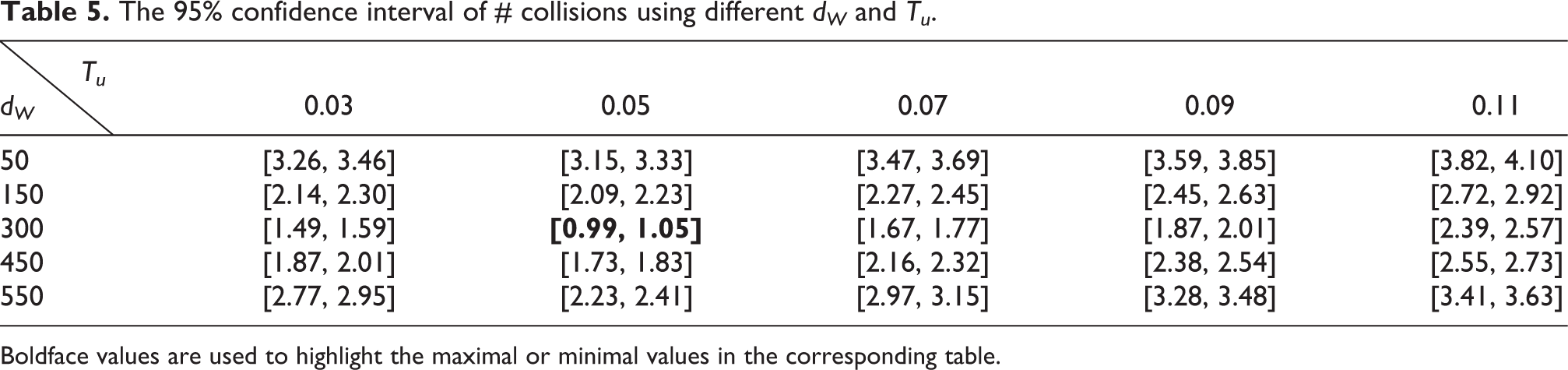
Boldface values are used to highlight the maximal or minimal values in the corresponding table.

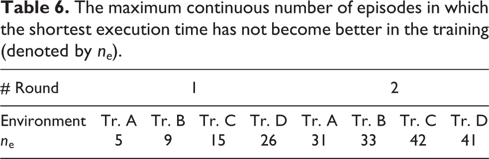
The curves of the execution time, the number of collisions, the number of coefficient changes, and the loss during the training process are shown in Figure 6. They were filtered by the moving average with a window size of 10. The points marked by “Tr. A, Tr. B,…” mean that the training was switched to the corresponding environments. We use a value called n_e to measure the skill that the agent has learned, as shown in Table 6. At the start of the training, the agent could not converge (the execution time was still decreasing when we switch the training). After the agent was trained in more environments, it starts learning with a shorter initial execution time and converges faster. This means our agent was learning continuously to optimize its performance in different types of task environments.

Figure 6.

(a to d) The training results under the setting of $d_{\text{W}}=0.05$ and $T_{\text{u}}=300$ .

Table 6.

The maximum continuous number of episodes in which the shortest execution time has not become better in the training (denoted by n_e ).

# Round	1				2
Environment	Tr. A	Tr. B	Tr. C	Tr. D	Tr. A	Tr. B	Tr. C	Tr. D
$n_{\text{e}}$	5	9	15	26	31	33	42	41

Test

To illustrate the generalization ability of the trained agent, we tested the agent trained with $d_{\text{W}}=0.05$ and $T_{\text{u}}=300$ in both the training environments and some previously unseen environments that were not used in the training. Note that our agent is a continuous RL model, so even in the test time, the weights of the trained NNs would be still updated. We compared the performance of this continuous learning agent with that of the fixed human-tuned coefficients and the performance of a noncontinuous learning agent. The noncontinuous learning agent was trained in the same way as the continuous one, but its NN would be fixed during the test time (it still changes the coefficients dynamically). Figure 7 shows the new test environments.

Figure 7.

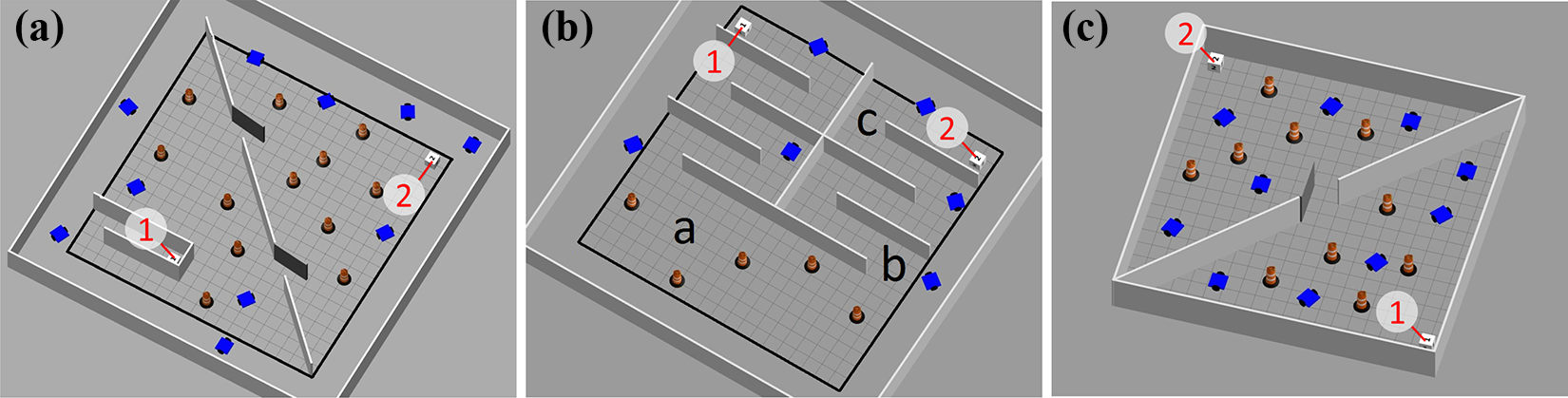
The test environments (note that the blue cars are unpredictable moving obstacles): (a) Te. A, (b) Te. B, and (c) Te. C.

1. In Te. A, the walls and the doors in the working zone are placed along the diagonal.

2. In Te. B, there is an area similar to a maze in the upper half of the working zone. It is less cluttered than the training environments, but the distance from the start to the goal is longer.

3. In Te. C, the working zone is directly bounded by walls. Both the robot and the moving obstacles can only move within the working zone, so that the robot will always work with 10 moving obstacles in this environment.

The test results are shown in Figure 8 and Tables 7 and 8. The performance measurements are the same as those in the training. We found that both the continuous learning agent and the noncontinuous learning agent outperformed the fixed human-tuned coefficients. Furthermore, the continuous learning agent significantly improves the performance of noncontinuous agent ( $p\ll 0.05$ from analysis of variance tests). The improvements are not only the reduced average navigation time to the goal but, more importantly, the significantly reduced average number of collisions during the navigation. Besides, the results have shown that our approach naturally transfers the knowledge learned in the training environments to completely different new environments. The differences can be the numbers of static and unknown moving obstacles or the structures of environments.

Figure 8.

(a to c) Average test results over 100 episodes.

Table 7.

The 95% confidence interval of execution time (s) in the test.

	Tr. A	Tr. B	Tr. C	Tr. D	Te. A	Te. B	Te. C
FHC	[38.95, 39.85]	[41.20, 42.00]	[42.84, 43.56]	[45.94, 47.06]	[44.24, 45.36]	[47.77, 48.83]	[46.60, 47.60]
NLA	[36.25, 36.55]	[36.94, 37.26]	[37.21, 37.59]	[37.63, 37.97]	[37.44, 37.76]	[40.58, 41.02]	[40.98, 41.42]
CLA	[35.32, 35.48]	[35.30, 35.50]	[36.12, 36.28]	[36.62, 36.78]	[36.16, 36.44]	[39.07, 39.33]	[39.32, 39.68]

FHC: fixed human-tuned coefficients; NLA: noncontinuous learning agent; CLA: continuous learning agent.

Boldface values are used to highlight the maximal or minimal values in the corresponding table.

Table 8.

The 95% confidence interval of # collisions in the test.

	Tr. A	Tr. B	Tr. C	Tr. D	Te. A	Te. B	Te. C
FHC	[3.94, 4.42]	[4.22, 4.62]	[4.03, 4.41]	[5.88, 6.20]	[4.87, 5.61]	[3.06, 3.70]	[6.48, 7.22]
NLA	[1.54, 1.72]	[1.68, 1.90]	[1.70, 1.86]	[1.64, 1.82]	[1.87, 2.09]	[1.71, 1.97]	[2.23, 2.49]
CLA	[0.38, 0.54]	[0.63, 0.79]	[0.54, 0.70]	[0.61, 0.77]	[1.03, 1.21]	[0.90, 1.06]	[1.00, 1.10]

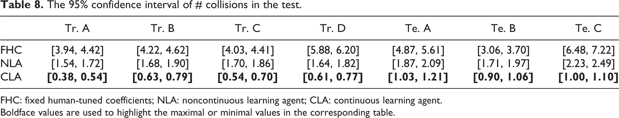
FHC: fixed human-tuned coefficients; NLA: noncontinuous learning agent; CLA: continuous learning agent.

Boldface values are used to highlight the maximal or minimal values in the corresponding table.

Table 9.

Average data with the standard deviation on the real robot experiments.

	Initial coefficients	Ending coefficients	# coefficients changes	Execution time (s)	Min. dist. to obs. (m)
No obstacles	$W_{\text{T}}=1,W_{\text{A}}=1,W_{\text{D}}=0.5$	$W_{\text{T}}=1,W_{\text{A}}=1,W_{\text{D}}=0.2$	15.8 ± 0.39	16.74 ± 0.21	N/A
Static only	$W_{\text{T}}=1,W_{\text{A}}=1,W_{\text{D}}=0.2$	$W_{\text{T}}=1,W_{\text{A}}=1,W_{\text{D}}=0.35$	19.1 ± 0.58	25.19 ± 0.47	0.42 ± 0.03
Mix	$W_{\text{T}}=1,W_{\text{A}}=1,W_{\text{D}}=0.35$	$W_{\text{T}}=1,W_{\text{A}}=1,W_{\text{D}}=0.35$	20.9 ± 0.83	26.44 ± 0.76	0.84 ± 0.08
Dynamic only	$W_{\text{T}}=1,W_{\text{A}}=1,W_{\text{D}}=0.35$	$W_{\text{T}}=1,W_{\text{A}}=1,W_{\text{D}}=0.4$	16.3 ± 0.72	21.30 ± 0.68	0.76 ± 0.07

Figure 9 shows the curves of the coefficients tuned by the continuous learning agent and the snapshots at three different time instants during one of the test episodes in Te. B. The corresponding places of the snapshots in Te. B are marked in Figure 7(b) to (d). The horizontal “plan number” means the number of planning cycles. At the start of the test episode, the values of the coefficients are set randomly. In snapshot (b), mixed static and dynamic obstacles are being dealt with. In this case, drastic orientation changes can easily result in collisions, and there is no space for the robot to keep far away from the obstacles. Hence, the penalties for the orientation change $\left(W_{\text{A}}\right)$ are increased with the decreased penalty for the distance to obstacles $\left(W_{\text{D}}\right)$ . In snapshot (c), the robot is navigating a maze-like area, where keeping away from the wall is the key to ensuring safety, and frequent turnings are necessary to pass through the maze. Therefore, the penalty for the distance to obstacles is increased and the penalties for the orientation change are decreased. In snapshot (d), the robot will arrive at the goal soon. Both the penalties for the orientation change and the distance to obstacles are decreased, which means that the importance of the time efficiency $\left(W_{\text{T}}\right)$ is increased. The robot now will move along a trajectory as short as possible to reach the goal.

Figure 9.

(a) Curves of coefficients and (b to d) snapshots during one of the test episodes in Te. B in the simulation (note that the blue cars are unpredictable moving obstacles).

Moreover, from the results we can tell that in the same environment, when using the RL agent to tune the coefficients of cost functions online, more frequent coefficient changes often result in more efficient and safer navigation. The frequency depends largely on the changes of the environment during navigation, such as the number of moving obstacles. For example, the number of moving obstacles in Te. C remains fixed all the time, so the number of coefficient changes needed in this environment is smaller than that in the other environments, even though the environment itself is cluttered. Note that if the number of the moving obstacles in the working zone is fixed and the obstacles move along fixed trajectories, the coefficients in the cost function will converge after training for some time. This means that the number of coefficient changes in such environments will be nearly zero after convergence, because both the number and the motion pattern of the obstacles become unchanged.

Real robot experiments

Real robot experiments were performed with a Turtlebot 2 platform. The experiments were ran on a sequence of 3.5 m² environments. As the robot traversed the environment, the continuous learning agent modified the coefficients at real-time until the robot reached the goal. For each subsequent environment, the initial coefficients were set to the final coefficients when the robot reached the goal in the previous environment.

The first environment contains no obstacles. The robot is easily able to move on a straight line to the goal. The second environment contains four static obstacles. The third environment contains two static obstacles and one dynamic obstacle moving on a straight line back and forth. The fourth environment contains two dynamic obstacles that move on straight line trajectories repeatedly and no static obstacles. An image for each environment containing obstacles is shown in Figure 10.

Figure 10.

Real robot environments. The dynamic obstacles move on straight lines back and forth repeatedly: (a) only static obstacles, (b) mixture of static dynamic obstacles, and (c) only dynamic obstacles.

Figure 11 shows how the coefficients change over time, while the robot is executing motion. In general, the $W_{\text{D}}$ coefficient (minimum distance to obstacles) changes significantly and often, but the $W_{\text{A}}$ coefficient (orientation change) changes only slightly. While moving in the presence of no obstacles, the $W_{\text{D}}$ coefficient decreases rapidly. For each new environment, the $W_{\text{D}}$ coefficient changes significantly throughout the run. The fluctuation of the $W_{\text{D}}$ coefficient is likely due to the robot having to perform more obstacle avoidance behavior while navigating obstacles, and then requiring less obstacle avoidance after it passes obstacles and approaches the goal.

Figure 11.

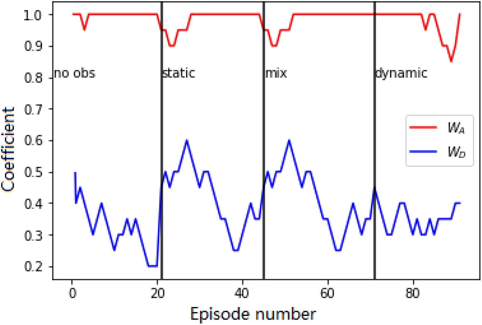
The values of the coefficients while the real robot is navigating environments. The vertical lines show when the robot begins a new environment.

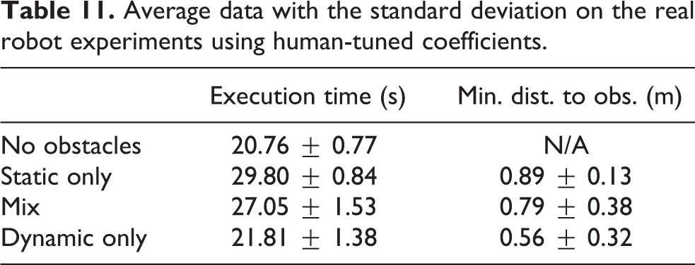
Comparing the results shown in Tables 9 and 10, under the RL agent, and in Tables 11 and 12, under manually tuned coefficient values, it is clear that the reinforcement agent results in more efficient and less conservative robot motion in the environment with static obstacles and safer motion in the environment with dynamic obstacles. Note that the RL agent was trained entirely in simulation and with different environments. No further training of the agent was done before running it in the real experiments. The purpose of this is to verify the agent’s ability of transferring the knowledge learned in the simulations to the real world. With further training of the agent in real experiments, we expect that the robot will have better performances.

Table 10.

The 95% confidence interval of data on the real robot experiments

	Initial coefficients	Ending coefficients	# coefficients changes	Execution time (s)	Min. dist. to obs. (m)
No obstacles	$W_{\text{T}}=1,W_{\text{A}}=1,W_{\text{D}}=0.5$	$W_{\text{T}}=1,W_{\text{A}}=1,W_{\text{D}}=0.2$	[15.72, 15.88]	[16.70, 16.78]	N/A
Static only	$W_{\text{T}}=1,W_{\text{A}}=1,W_{\text{D}}=0.2$	$W_{\text{T}}=1,W_{\text{A}}=1,W_{\text{D}}=0.35$	[18.98, 19.22]	[25.09, 25.29]	[0.41, 0.43]
Mix	$W_{\text{T}}=1,W_{\text{A}}=1,W_{\text{D}}=0.35$	$W_{\text{T}}=1,W_{\text{A}}=1,W_{\text{D}}=0.35$	[20.73, 21.07]	[26.28, 26.60]	[0.82, 0.86]
Dynamic only	$W_{\text{T}}=1,W_{\text{A}}=1,W_{\text{D}}=0.35$	$W_{\text{T}}=1,W_{\text{A}}=1,W_{\text{D}}=0.4$	[16.15, 16.45]	[21.16, 21.44]	[0.75, 0.77]

Table 11.

Average data with the standard deviation on the real robot experiments using human-tuned coefficients.

	Execution time (s)	Min. dist. to obs. (m)
No obstacles	20.76 ± 0.77	N/A
Static only	29.80 ± 0.84	0.89 ± 0.13
Mix	27.05 ± 1.53	0.79 ± 0.38
Dynamic only	21.81 ± 1.38	0.56 ± 0.32

Table 12.

The 95% confidence interval of data on the real robot experiments using human-tuned coefficients

	Execution time (s)	Min. Dist. to Obs. (m)
No obstacles	[20.60, 20.92]	N/A
Static only	[29.63, 29.97]	[0.86, 0.92]
Mix	[26.74, 27.36]	[0.71, 0.87]
Dynamic only	[21.53, 22.09]	[0.49, 0.63]

Conclusions

We have introduced a utility-based multi-objective continuous learning framework utilizing a real-time motion planner to make a robot continuously learn how to adapt online multi-objective optimization for robot motion. We focus on improving and testing our framework for continued learning and adaptation in changing dynamic environments. Moreover, by the simultaneous robot motion and continuous coefficient-update model learning, our framework enables the robot to self-tune its behavior online to constantly adapt to unknown changes in task environments with ever improved performance. The effectiveness and practicality of the proposed framework have been demonstrated by a case study with the RAMP, through both the simulations and the real robot experiments in various dynamic environments. In comparison with the human-tuned coefficients, the proposed framework improved the execution time about 17% on average in the simulations and 10% on average in the real robot experiments. The encouraging results verify the performance gain in the robot navigation from our framework and the transferability of the trained agent from training environments to unseen environments, and even from simulation to real environments. As such, the trained agent acquires a general ability for effective navigations in different environments.

The application of the proposed framework is not restricted to the case study with RAMP shown in this article. Our framework can accommodate other real-time motion planners and enable stability and intelligence for the robot navigation. In the real-time motion planning problem of mobile robots, the role of RL is making decisions at a semantic level for the robot navigation. One of the ways to make such decisions is tuning the behavioral multi-objective coefficients online based on the performance-driven feedback. In this way, the RL agent is able to determine the time-varying preferences among different objectives at different navigation time.