Sage Journals: Discover world-class research

Abstract

Ant colony algorithm or artificial potential field is commonly used for path planning of autonomous vehicle. However, vehicle dynamics and road adhesion coefficient are not taken into consideration. In addition, ant colony algorithm has blindness/randomness due to low pheromone concentration at initial stage of obstacle avoidance path searching progress. In this article, a new fusion algorithm combining ant colony algorithm and improved potential field is introduced making autonomous vehicle avoid obstacle and drive more safely. Controller of path planning is modeled and analyzed based on simulation of CarSim and Simulink. Simulation results show that fusion algorithm reduces blindness at initial stage of obstacle avoidance path searching progress and verifies validity and efficiency of path planning. Moreover, all parameters of vehicle are changed within a reasonable range to meet requirements of steering stability and driving safely during path planning progress.

Keywords

Autonomous vehicle path planning fusion algorithm (improved ant colony algorithm (IACA)improved artificial potential field (IAPF))road adhesion coefficient environment perception pheromone update

Introduction

Statistics show that traffic accidents account for 90% of safety accidents around the world, among which more than 80% casualties were confirmed in traffic accidents.¹ For autonomous vehicle, an effective and stable obstacle avoidance path planning algorithm plays an important role in reducing such accidents significantly.

To some extent, obstacle avoidance path planning of autonomous vehicle is similar to obstacle avoidance robots. Vehicle dynamics, traffic regulations, and road adhesion coefficient should also be considered when it comes to obstacle avoidance path planning for autonomous vehicle. Main advanced path planning methods applied for autonomous vehicle are artificial potential field model,^2

–5 Dijkstra algorithm, ant colony algorithm and particle swarm optimization, and so on.⁶ Fast algorithms are presented by Nash et al. for discrete state spaces, but those algorithms tend to produce paths of which nonlinear constraint of autonomous vehicle is taken into account.⁴ Jia et al.⁷ introduce a model predictive path tracking controller to consider effects of vehicle dynamics and actuators’ limitations in path tracking, which can be used to solve problems that the planned path is not feasible to be traced by autonomous vehicle.

A new fusion method combining ant colony algorithm and improved potential field that is used for path planning is proposed in this article.⁸ An appropriate path which considering the constraint of vehicle dynamics, traffic regulations, and road adhesion coefficient can be planned by using this fusion method. In the initial stage of path planning, pheromone concentration used for path searching is insufficient, transfer probability function of ant colony algorithm is adjusted by introducing improved potential field as heuristic information, and weight is introduced to consider influence of road adhesion coefficient and vehicle speed on choice of path. Role of improved potential field reduces gradually, pheromone concentration and function of heuristic information start to work with deepening of path planning process. Research results show that the new fusion method can reduce the number of iterations used in path searching progress, avoid stagnation and blindness in initial stage, and improve the efficiency of path planning for autonomous vehicle.

Typical structure of autonomous vehicle is shown in Figure 1. It consists of three parts, including external sensors, control system, and actuators. Risk of traffic accidents will be found reasonably by using external sensors like camera, millimeter wave radar, high-definition map, and Global Positioning System. Control system of autonomous vehicle can be divided into planning layer and control layer. Reasonable decisions will be made by planning layer according to the data of external sensors, and then instructions will be transmitted to actuators by control system.

Figure 1.

Typical structure of autonomous vehicle.

In the second section, methods that extract image information in process of environmental perception are presented. In the third section, path planning considering vehicle dynamic, traffic regulation, and road adhesion coefficient is planned by fusion method. In the fourth section, obstacle avoidance path planning system is evaluated with a high-fidelity CarSim simulation and the results are presented and discussed. The fifth section concludes the article.

Environment perception

Detecting environmental information around autonomous vehicle is of great importance to path planning in complex and dynamic environment.⁹ Current research shows that environmental perception based on single external sensor is restricted by less information and more complex algorithm, which is difficult to satisfy the requirements of real-time detection and high robustness during driving process. Therefore, multi-sensor (camera and radar) fusion technology¹⁰ is used to make up the limitation of single sensor, especially in complex and dynamic environment. Meanwhile, robustness of path planning algorithm would be improved. Figure 2 shows the outline of fusion system between radar and vision.

Figure 2.

Outline of radar and vision fusion system.

Methods will be used to unify data obtained by different sensors into same coordinate system for increasing the accuracy of information fusion. Detected environmental information was extracted into global coordinate system through coordinate transformation, so as to confirm the position of obstacles (pedestrians, vehicles, etc.) in real time. Coordinate system of radar, camera and their projection coordinate system are established respectively. radar detection plane is perpendicular to the longitudinal axis of the vehicle,optical axis of the camera is parallel to longitudinal axis of the vehicle after calibration. Figure 3 shows the schematic diagram of coordinate conversion. Location of obstacles confirmed by sensors will be converted to image coordinate system by the following formula¹¹

Figure 3.

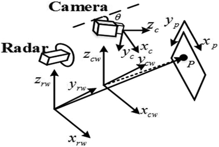
Coordinates conversion of radar and camera.

{\begin{matrix} x_{p} = c_{x} + \frac{(x_{r ω} - l_{x}) f}{h sin θ + (y_{r ω} + l_{y}) cos θ} \\ y_{p} = c_{y} + \frac{[hcosθ - (y_{r ω} + l_{y}) sin θ] f}{h sin θ + (y_{r ω} + l_{y}) cos θ} \end{matrix}

In equation (1), c_x and c_y denote offset of axis, f is focus distance of camera, l_x is distance between radar projection coordinate system and x-axis in world coordinate system, l_y is distance between radar projection coordinate system and y-axis in world coordinate system, h is height of camera installation, and θ is pitching angle of camera.

It is known to us that region of interest refers to areas which represent image content mostly, and plays an important role in image processing. Features of image detected by sensor during environmental perception progress are vividly shown in Figure 4.

Figure 4.

Features extraction.

In Figure 4, different color boxes are used to mark vehicles, pedestrians, bicycles, and so on. All above-marked image information make preparation for confirming the distance between obstacle and autonomous vehicle.

Path planning

A new path considering vehicle dynamic, road structure, traffic regulation, and road adhesion coefficient is planned by fusion method.

Vehicle dynamic model

The main purpose of this part is to make autonomous vehicle manipulate accurately and steadily, so calculation time of control algorithm is reduced by neglecting influence of suspension factors and simplifying dynamic model. Vehicle dynamic model¹² with two degrees of freedom (DOF) contains most of motion characteristics of vehicle in actual driving process. Notation used in vehicle dynamic model is shown in Figure 5.

Figure 5.

Vehicle dynamic model with two DOF. DOF: degrees of freedom.

It is assumed that autonomous vehicle relies on front wheels for steering, and motion equations of vehicle dynamic model with two DOF are

\begin{array}{l} m (\dot{u} - v γ) = F_{x T} \\ m (\dot{v} + u γ) = F_{f} cos δ + F_{r} \\ I_{z} \dot{γ} = a F_{f} cos δ - b F_{r} \end{array}

In equation (2), v, u, and γ denote lateral velocity, longitudinal velocity, and yaw rate of vehicle; $F_{x T}$ is longitudinal resultant force of tire; F_f and F_r are lateral force of front and rear tire, respectively; m is mass of vehicle; and I_z is inertial momentum of automobile around OZ-axis. Considering angle of front wheel δ is small, formula (2) can be further expressed as following types

\begin{array}{l} m (\dot{v} + u γ) = C_{f} α_{f} + C_{r} α_{r} \\ I_{z} \dot{γ} = a C_{f} α_{f} - b C_{r} α_{r} \end{array}

In equation (3), $α_{f}$ and $α_{r}$ denote sideslip angle of front and rear tire. C_f and C_r are cornering stiffness of front and rear tire, respectively. A linear tire model is used for lateral tire forces¹³

\begin{array}{l} F_{f} = C_{f} α_{f} = C_{f} (β + \frac{a γ}{u} - δ) \\ F_{r} = C_{r} α_{r} = C_{r} (β - \frac{b γ}{u}) \end{array}

Differential equation of vehicle motion with two DOF is obtained as follows

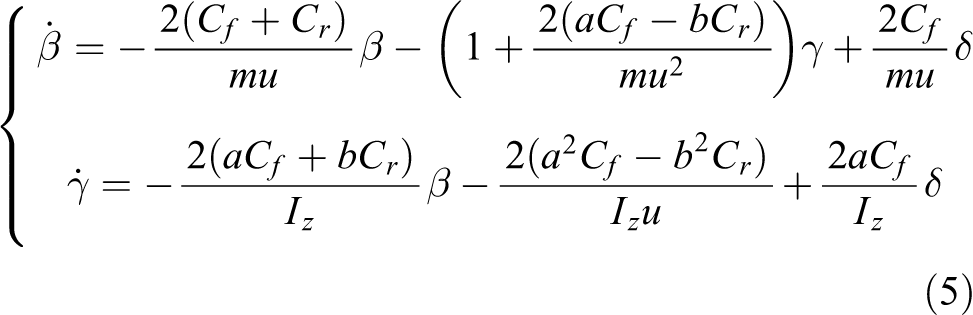
{\begin{matrix} \dot{β} = - \frac{2 (C_{f} + C_{r})}{m u} β - (1 + \frac{2 (a C_{f} - b C_{r})}{m u^{2}}) γ + \frac{2 C_{f}}{m u} δ \\ \dot{γ} = - \frac{2 (a C_{f} + b C_{r})}{I_{z}} β - \frac{2 (a^{2} C_{f} - b^{2} C_{r})}{I_{z} u} + \frac{2 a C_{f}}{I_{z}} δ \end{matrix}

Vehicle linear dynamics can then be obtained by linearizing equations (2) to (5)

\dot{x} = A x + B δ, x = {[\begin{matrix} β & γ \end{matrix}]}^{T}

In equation (6), δ is input parameter, x is state vector, A is state matrix, and B is input matrix.

The above vehicle dynamic model with two DOF is discretized by zero-order hold method and utilized for model predictive path planning controller.

Estimation algorithm for adhesion coefficient

According to typical road μ-s curves shown in Figure 6, road adhesion coefficient reaches peak when slip rate is about 0.16, which is called peak adhesion coefficient of pavement. In addition, there are some differences between different types of pavement. For snow- and ice-covered road, the relationship between adhesion coefficient and slip rate is relatively smooth, besides the available adhesion condition of road surface is also small.¹⁴

Figure 6.

Schematic diagram of pavement adhesion coefficient estimation.

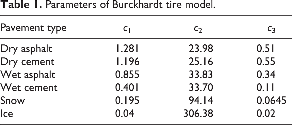
Chang-gang et al. fitted a semi-empirical road and tire mathematical model by computer simulation.¹⁵ Expression of this model is shown as follows

μ (s) = c_{1} (1 - e^{- c_{2} x}) - c_{3} s

In equation (7), μ denotes road adhesion coefficient; s is slip rate; and c ₁, c ₂, and c ₃ denote constant value obtained by fitting. Table 1 shows Burckhardt tire model parameters.

Table 1.

Parameters of Burckhardt tire model.

Pavement type	c ₁	c ₂	c ₃
Dry asphalt	1.281	23.98	0.51
Dry cement	1.196	25.16	0.55
Wet asphalt	0.855	33.83	0.34
Wet cement	0.401	33.70	0.11
Snow	0.195	94.14	0.0645
Ice	0.04	306.38	0.02

It is necessary to know the potential peak adhesion coefficient of current road in order to obtain the maximum road adhesion. On the basis of Burckhardt model, variation range of peak adhesion and optimal slip rate for six typical pavements are obtained by computer simulation, as shown in Table 2.

Table 2.

Peak adhesion coefficient of six typical pavements.

Pavement type	Range	Average	Optimal slip rate
Dry asphalt	0.85–0.98	0.92	0.85–0.93
Dry cement	0.88–1.0	0.95	0.85–0.93
Wet asphalt	0.62–0.78	0.70	0.62–0.85
Wet cement	0.75–0.8	0.78	0.62–0.85
Snow	0.2–0.28	0.24	0.1–0.20
Ice	0–0.1	0.10	0.1–0.20

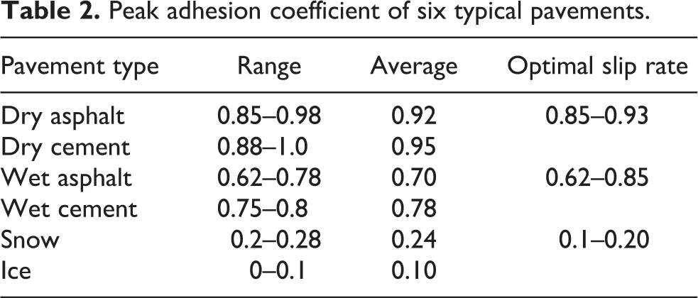
In this way, adhesion coefficient can be estimated based on typical road surface which is more similar to tested road surface. Based on the idea of analogy, the relationship between peak adhesion coefficients is presented as follows

μ_{road} = λ_{1} \frac{φ}{φ_{1}} μ_{1 max} + λ_{2} \frac{φ}{φ_{2}} μ_{2 max} + λ_{3} \frac{φ}{φ_{3}} μ_{3 max} + λ_{4} \frac{φ}{φ_{4}} μ_{4 max}

In equation (8), $λ_{1}$ , $λ_{2}$ , $λ_{3}$ , and $λ_{4}$ denote analogical coefficient, derived from four directions (45°, 135°, 225°, and 315°) on contact surface of wheel. φ is current pavement adhesion coefficient, $μ_{1 max}$ , $μ_{2 max}$ , $μ_{3 max}$ , and $μ_{4 max}$ denote peak adhesion coefficient of typical pavement nearby. $φ_{1}, φ_{2}, φ_{3}, and φ_{4}$ are adhesion coefficient of adjacent pavement, respectively. The above parameters will meet the following relationship: $φ_{1} < φ_{2} < φ < φ_{3} < φ_{4}$ .

Improved potential field

Artificial potential field method was first proposed by Khatib and applied to robot local path planning¹⁶ in the 1990s. It is a field generated by road structure, traffic regulations, and target goal to lead autonomous vehicle toward destination.

Figure 7 gives schematic diagram of partial path planning under multiple restrained conditions. Path planning is affected by gravitation model of multi-category objects while satisfying traffic regulations and vehicle characteristics. The functions presented below are explicit introduction of two types of virtual gravitation model and one kind of virtual repulsion model.

Figure 7.

Path planning under multiple restrained conditions.

Gravity model of safety lane change:

Vehicle needs to change lanes when there are traffic participants ahead or other conditions that hinder normal driving in process of traveling

F_{a - c} = {\begin{array}{l} (1 - \int_{- β}^{β} \int_{0}^{t} \frac{v (t) sin β (t) t}{S_{lane 1 - 2}} d t d β) μ_{slide} m g, con = 1 \\ 0, con = 0 \end{array}

In equation (9), $v (t)$ is relationship between speed and time, $β (t)$ is relationship between sideslip angle of vehicle centroid and time, $S_{lane 1 - 2}$ is midline distance between current lane and changed lane, m is vehicle’s mass, con is judgment condition of safe lane changing, and $con = 1$ denotes lane changing allowable.

This article sets up different driving modes and observes change of vehicle parameters to verify the validity of lane changing model, with simulation of CarSim and Simulink. Simulation parameters are set as follows: frontal area (A) of vehicle is 1.6 m², drag coefficient (f_w ) is 0.3, the rolling resistance coefficient (f_r ) of vehicle is 0.014, and road adhesion coefficient ( $μ_{road}$ ) is 0.85.

Vehicle travels at speed of 30 km h⁻¹, 50 km h⁻¹, and 100 km h⁻¹, respectively. Lane changing operation is carried out under the effect of lane changing gravity. Figure 8 shows changes of vehicle characteristic.

Figure 8.

(a) Curve of vehicle trajectory, (b) curve of steering, and (c) curve of lateral acceleration.

As shown in Figure 8, the trajectory of vehicle is smooth, which makes vehicle stability. Lateral acceleration changes from −0.15 g to 0.15 g and the steering wheel angle decreases with increase of vehicle speed, which ensures vehicle travels more safety and provides better driving experience.

2. Virtual gravity model of global route

F_{a - g} (t) = f_{a - g} (μ_{roll} m g + \frac{1}{16} A C_{w} v^{2} (t)), threat = 0

In equation (10), $f_{a - g}$ is gravity coefficient of global planning route, $μ_{roll}$ is coefficient of rolling resistant, m is vehicle’s mass, C_w is aerodynamic drag coefficient, A is frontal area of vehicle, v is vehicle’s speed, and $threat = 0$ denotes without threat.

Vehicle travels in descent direction of potential gradient with 40 km h⁻¹ speed. Speed limits of front section are 80 km h⁻¹ and 40 km h⁻¹, respectively. Changes of longitudinal speed and acceleration are shown in Figure 9 under the influence of global gravitation.

Figure 9.

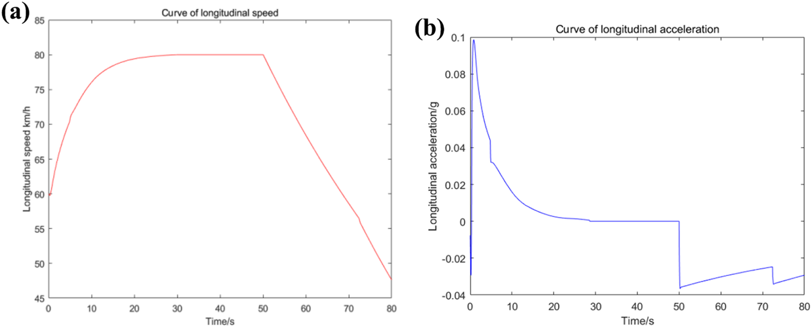
(a) Curve of longitudinal speed and (b) curve of longitudinal acceleration.

As shown in Figure 9, under influence of global gravitation, vehicle accelerates to reach speed of 80 km h⁻¹ gradually, alters to deceleration after speed limit changes to 40 km h⁻¹. Virtual gravitation of global planning can guide vehicle travels with the speed approaching to current limit.

3. Virtual repulsion model of lateral direction

F_{r - y} = {\begin{array}{l} f_{r - y} \frac{{\tilde{v}}_{y} \cdot μ_{road} \cdot m \cdot g}{v sin β (t) {\tilde{S}}_{y}^{2}} \begin{matrix} , & {\tilde{S}}_{y} < S_{safe - y} \end{matrix} \\ 0, {\tilde{S}}_{y} > S_{safe - y} \end{array}

In equation (11), $f_{r - y}$ is coefficient of lateral obstacles’ (guardrail, bushes, etc.) repulsion force on vehicle, ${\tilde{v}}_{y}$ is relative speed between lateral obstacle and ego vehicle, $v sin θ (t)$ is relationship between lateral component of speed and time, $β (t)$ is relationship between sideslip angle of vehicle centroid and time, ${\tilde{S}}_{y}$ is relative distance between vehicle and nearest object on vehicle’s either side, $μ_{road}$ is identification of road adhesion coefficient, and $S_{safe - y}$ is safe distance needed for autonomous vehicle to avoid collision with lateral obstacles.

Road structure Potential field (PF) is typical case of virtual repulsion model in lateral direction; it is defined with quadratic functions, and their gradients increase linearly with reduction of safe distance. The further the vehicle deviates from road center line, the greater the virtual potential field repulsion force of road boundary. Figure 10 shows road boundary repulsion model of lateral direction.

Figure 10.

Road boundary repulsion model of lateral direction.

Consequently, it is important to verify the validity of established model under the influence of road boundary repulsion, with simulation of CarSim and Simulink.¹⁷ Figure 11 shows some results partial.

Figure 11.

(a) Curve of longitudinal speed, (b) curve of acceleration change, and (c) curve of steering wheel angle.

We can conclude from Figure 11 that vehicle position is corrected by road boundary repulsion constantly, making vehicle travel along the path, avoiding occurrence of deviating from the lane.

4. Virtual repulsion model of traffic lamp

\begin{array}{l} F_{r - l} = {\begin{array}{l} f_{r - light} \frac{M_{light}}{{\tilde{v}}_{i - light}} {(\frac{S_{safe}}{{\tilde{S}}_{light}})}^{2} μ_{road}, 0 < {\tilde{S}}_{light} \leq S_{safe} \\ 0, {\tilde{S}}_{light} > S_{safe} \end{array} \\ M_{light} = {\begin{cases} 1, (\frac{D}{V} > t_{g - r}) ∥ (l_{state} = 1) \\ 0, (\frac{D}{V} \leq t_{g - r}) & (l_{state} = 0) \end{cases} \end{array}

In equation (12), $f_{r - light}$ is repulsion coefficient of traffic lights, $M_{light}$ is information of traffic lamp, $M_{light} = 1$ denotes traffic signal light is red, ${\tilde{v}}_{i - light}$ is relative speed between traffic light and ego vehicle, $S_{safe}$ is minimum distance that vehicle can stop before halting, ${\tilde{S}}_{light}$ is relative distance between traffic light and ego vehicle, and $μ_{road}$ is identification of road-tire adhesion coefficient.

In order to verify the validity of established model, some parameters in simulation are set as follows: distance between vehicle and traffic light is 100 m, the influence range of signal lamp is 40 m, and vehicle moves at constant speed of 50 km h⁻¹.

As shown in Figure 12, the vehicle will glide and decelerate under the influence of rolling resistance. Braking system of the vehicle starts to work after entering the range which is affected by virtual repulsion of traffic lights. Evidently, vehicle speed drops rapidly, completes braking before reaching the station of signal lamp.

Figure 12.

(a) Curve of distance between vehicle and traffic lamp, (b) curve of longitudinal speed, and (c) curve of longitudinal acceleration.

5. Virtual repulsion model of front participants

F_{r - f} = {\begin{array}{l} f_{r - f} \frac{{\tilde{v}}_{front} \cdot μ_{road} \cdot m \cdot g}{v (t) cos β (t) {\tilde{S}}_{front}^{2}}, 0 < {\tilde{S}}_{front} \leq S_{safe-front} \\ 0, {\tilde{S}}_{front} \geq S_{safe-front} \end{array}

In equation (13), $f_{r - f}$ is repulsion coefficient of front vehicle to ego vehicle, $μ_{road}$ is identification of front road adhesion coefficient, $v (t)$ is relationship between speed and time, $β (t)$ is relationship between sideslip angle of vehicle centroid and time, ${\tilde{v}}_{front} (t)$ is relative speed between front obstacle and ego vehicle, ${\tilde{S}}_{front}$ is distance between front obstacle and ego vehicle, and $S_{safe-front}$ is safe distance that is needed for avoiding collision between front obstacle and ego vehicle.

In order to verify the validity of established model, some parameters in simulation are set as follows: speed of front traffic participants is 20 km h⁻¹, distance between ego vehicle and front traffic participants is 60 m, and vehicle travels along the path with speed of 80 km h⁻¹. Changes of vehicle characteristic are shown in Figure 13.

Figure 13.

(a) Curve of distance between ego vehicle and front vehicle and (b) curve of longitudinal speed.

As shown in Figure 13, virtual repulsion force of front participants is greater than gravity force of global route when distance between ego vehicle and front vehicle is less than the threshold value specified by safe distance model. Consequently, vehicle decelerates the speed to keep a safety distance from front participants so as to avoid collision, vice versa.

Path planning

Improvement of transfer probability function

Transfer probability function of basic ant colony algorithm that is applied to path problem is

P_{m n}^{k} (t) = {\begin{array}{l} \frac{τ_{m n}^{α} (t) η_{m n}^{β} (t)}{\sum_{j \in allowed k (t)} τ_{m j}^{α} (t) η_{m j}^{β} (t)}, n \in allowed k (t) \\ 0, else \end{array}

\begin{array}{l} η_{m n}^{β} (t) = 1 / d_{m n} \\ τ_{m n} (t + δ) = (1 - ρ) τ_{m n} (t) + Δ τ_{m n} \end{array}

\begin{array}{l} Δ τ_{m n} = \sum_{k = 1} Δ τ_{m n}^{k} \\ Δ τ_{m n}^{k} (t, t + δ) = {\begin{array}{l} Q / L_{k}, ant k passes  through (m, n) \\ 0, else \end{array} \end{array}

In equations (14) to (16), $η_{m n}^{β} (t)$ is function of distance heuristic information, $τ_{m n} (t)$ indicates pheromone concentration at node j, α is factor of pheromone concentration, β is factor of heuristic information, $allowed k (t)$ is next available node after accessed node has been removed, $ρ (0 < ρ < 1)$ denotes volatility coefficient of pheromone concentration, $Δ τ_{m n}$ is increment of pheromone concentration between (m, n), and L_k is length of path.

In initial stage of path planning, pheromone concentration used for path search is insufficient. Drivable path waiting for selection is obtained by using improved potential field algorithm, vehicle travels along the path with the fastest descent of potential field force gradient due to resultant force of improved potential field. With deepening of path planning, pheromone concentration on searching path reaches the threshold value, the role of improved potential field is reduced. In order to reduce blindness/randomness and avoid stagnation at initial stage of path planning, Path searched by ant colony algorithm according to the path enlightened by artificial potential field algorithm. The entire process can be described with the following flowchart (Figure 14).¹⁸

Figure 14.

Flowchart of fusion algorithm.

Resultant force of improved potential field which is established under multiple constraints is formulated as follows

F_{total} = F_{a - c} + F_{a - g} + F_{r - f} + F_{r - y} + F_{r - l}

Transfer probability function of ant colony algorithm is adjusted by introducing resultant force of improved potential field as heuristic information, weight is introduced to consider the influence of road adhesion coefficient and vehicle speed on choice of path. Information function enlightened by resultant force of improved potential field is formulated as follows

η_{F}^{γ} (t) = \frac{k_{max} - k}{k_{max}} \cdot a^{F_{total} \cdot cos θ} \cdot (c_{1} \cdot μ_{road} + c_{2} \cdot l_{v})

In equation (18), γ is factor of heuristic information; $K_{max}$ denotes maximum iteration; K is current iteration; $a > 1$ and is constant; $F_{total}$ indicates resultant force of potential field; θ represents angle between potential field resultant force and optional path direction, the smaller the angle, the greater the $η_{F}^{γ} (t)$ ; c ₁ and c ₂ represent weight coefficient; $μ_{road}$ is identification of road-tire adhesion coefficient; and l_v is rank of vehicle speed

l_{v} = {\begin{array}{l} A, v > 60 \\ B, 30 \leq v \leq 60 \\ C, v < 30 \end{array}, {unit:km h}^{- 1}

Transfer probability function of ant colony algorithm is improved as follows

p_{m n}^{k} (t) = {\begin{array}{l} \frac{τ_{m n}^{α} (t) η_{m n}^{β} (t) η_{F}^{γ} (t)}{\sum_{j \in a l l l o w k (t)} τ_{m j}^{α} (t) η_{m j}^{β} (t) η_{F}^{γ} (t)}, n \in a l l o w k (t) \\ 0, else \end{array} (20)

Adjustment of pheromone update strategy

Ants will release pheromone on entire trajectory after completing one path searching loop. Not only global path but also local path needs are to be considered when it comes to pheromone update. It is necessary to adjust or replan local path due to real-time changes of driving information currently, such as traffic accidents, congestions, and other situations. This article improves pheromone update rule of basic ant colony algorithm,¹⁹ introduces pheromone update strategy of local path. Adjust pheromone update strategy dynamically based on convergence results of path search.

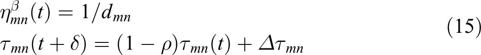
Updating rules of pheromone globally from point S to point E are as follows

τ_{S E} (t + 1) = {(1 - ρ)}^{ζ} τ_{S E} (t) + ρ Δ τ_{S E} (t, t + 1) + Δ τ_{S E}^{*}

\begin{array}{l} Δ τ_{S E} (t, t + 1) = \sum_{k = 1}^{m} Δ τ_{S E}^{k} (t, t + 1) \\ Δ τ_{S E}^{k} (t, t + 1) = {\begin{array}{l} Q / T_{k}, Vehicle k passes (m, n) \\ 0, else \end{array} \\ Δ τ_{S E}^{*} = {\begin{array}{l} σ \cdot Q / T_{k}, (m, n) is  global  optimal \\ 0, else \end{array} \end{array}

In equation (22), denotes volatilization coefficient of pheromone in global path. Q is pheromone concentration that determines the convergence rate of algorithm; T_k is the time which vehicle travels current path; represents extra pheromones added after elite vehicles travel from point S to point E; σ is number of elite vehicles.

Updating rules of local pheromone are as follows

τ_{m n} (t + 1) = {(1 - ε)}^{(1 - ξ)} τ_{m n} (t) + ε Δ τ_{m n}, t \in f (t)

Δ τ_{m n} = {\begin{array}{l} 1 / (T_{m n} + W_{n}), (m, n) is  global  optimal \\ 0, else \end{array}

In equation (24), $ε (0 < ε < 1)$ denotes volatilization coefficient of local pheromone; $T_{m n}$ is travel time of (m, n); $T_{delay}$ is delay-waiting time due to traffic congestion; W_n is passing time of signal intersection; $ζ = N_{s} - N_{0}$ ,N_s is convergence counter, N ₀ is constant integer; when $N_{s} < N_{0}$ , means $ζ < - 1$ , fusion algorithm converges slowly, strengthens role of pheromone update globally and reduces pheromone update locally; when $N_{s} > N_{0}$ , means $ζ > 1$ , fusion algorithm converges fastly, strengthens role of pheromone update locally and reduces pheromone update globally.

Results

Test scenarios

As is known to all, roads are complex and dynamic environments with obstacles moving at different speeds in different lanes and positions. Road itself might be curved, and lane might end or begin. Moreover, autonomous vehicle might be required to change its lane to take an exit or turn.¹⁹ Some normal scenarios for an autonomous driving assistance system are:

lane keeping on structured road;

lane changing with no obstacle in vicinity;

keeping a desired distance between front and rear vehicle.

In this article, two test scenarios are constructed to evaluate the performance of path planning based on fusion algorithm, including no traffic accident risk scenario and existence of traffic accident risk on planned path, respectively. Autonomous vehicle should be able to predict movement trend of obstacles and avoid accidents while keeping its lane, which is performed by keeping an appropriate distance from obstacles via accelerating/decelerating or steering. In general, the above conditions are appropriate for evaluating the performance of path planning system on basis of observing road structures, safety-traffic regulations, obstacle avoidance, and lateral maneuverability. The following two test scenarios are defined based on the above conditions.^20,21 Figure 9 shows schematic diagram of two typical test scenarios.

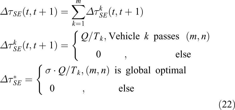
In scenario 1, autonomous vehicle will drive in a structured road environment and its lane ends in 650 m. Vehicle coordinate system is established based on center of gravity (COG). Shield non-approach repulsive force in lateral direction according to the shield theory. Lane keeping capacity and force acting on autonomous vehicle under virtual artificial potential field are analyzed. As is shown in Figure 15(a), virtual gravity acts on the point of P at the extension line of vehicle longitudinal axis.

Figure 15.

(a) Without traffic accident risk and (b) existence of traffic accident risk.

According to the formula of virtual repulsion and gravitation, the force and moment models shown in the following expressions are established

{\begin{array}{l} F_{x} (t) = F_{a - p} (t) cos α - F_{r} \\ F_{y} (t) = F_{r - y - 2} (t) - F_{r - y - 1} (t) + F_{a - p} (t) sin α \\ γ (t) I_{i} = (F_{r - y - 2} (t) - F_{r - y - 1} (t)) L_{x} + F_{a - p} (t) S_{p} sin α \end{array}

In equation (25), α is angle (point p) between virtual gravity and longitudinal axis of autonomous vehicle, $γ (t)$ is yaw rate of vehicle’s COG, and $I_{i}$ is rotary inertia of autonomous vehicle.

Lateral virtual repulsion force plays an important role in keeping autonomous vehicle in its lane. During driving process, yaw rate of vehicle should be controlled within a reasonable range. In order to prevent overlap of lateral repulsive forces produced by different types of objects from causing unreasonable lateral movement of autonomous vehicle, shielding idea is used to shield lateral virtual repulsion produced by non-approach objects, and only virtual repulsion which is produced by objects in vehicle vicinity will be retained. By analyzing the relationship between yaw rates and steering angle, lane keeping and planning function of steering system under lateral virtual repulsion is established as follows

F_{r - y - 2} (t) - F_{r - y - 1} (t) + F_{a - p} (t) = m a_{y}

Gao et al.²⁰ evaluate yaw rate based on multiple signals of wheel speed

γ_{0} (t) = \frac{(ω_{l} - ω_{r}) r_{0}}{B cos θ_{w}}, \begin{matrix} γ (t) = K (a_{y}) γ_{0} (t) \end{matrix}

In equation (27), $γ_{0} (t)$ is estimated value of yaw rate; $ω_{l}$ is angular velocity of left wheel of front axle, $ω_{r}$ is angular velocity of right wheel of front axle; r ₀ is wheel radius at static state; B is wheelbase of front axle; $θ_{w}$ is steering angle of front wheel. On the basis of formula (27), lateral acceleration signal is introduced to correct variation of wheel radius which is caused by internal and external wheel loads. Coefficient of correction (K) is generated and initial yaw rate $γ_{0} (t)$ is revised to obtain final estimated yaw rate $γ (t)$

γ (t) = K (a_{y}) \frac{(ω_{l} - ω_{r}) r_{0}}{B cos (θ_{steering} (t) / 10)}

In equation (28), $γ_{0} (t)$ is estimated value of yaw rate; $ω_{l}$ is angular velocity of left wheel of front axle, $ω_{r}$ is angular velocity of right wheel of front axle; r ₀ is wheel radius at static state; B is wheelbase of front axle; $θ_{w}$ is steering angle of front wheel.

In scenario 2, due to lack of observation, pedestrians or cyclist appeared in front of autonomous vehicle suddenly. Typical braking process is that drivers will perceive surrounding environment through vision, hearing, and other feeling, realizing that braking should be carried out under emergency situation, and then put down brake pedal for emergency braking until the autonomous vehicle stops. Safe distance model of this process is

S_{safe} = v_{r} t_{d} + \frac{v_{r}^{2}}{2 a_{max}} + d_{0}

In equation (29), $S_{safe}$ is safe distance; t_d is hysteresis time of braking, with value of approximately 1.2–2.0 s; $a_{max}$ is maximum deceleration of ego vehicle, with value of approximately 6–8 m s⁻²; v_r is speed of ego vehicle before braking; and d ₀ is distance between front vehicle and ego vehicle, with value of approximately 2–5 m.

It is known to us that collision cannot be avoided if distance between pedestrians, bicycles, and ego vehicle is less than minimum safety distance. At this point, a signal of steering control must be applied, and autonomous vehicle should choose an obstacle-free path to avoid collision by controlling steering operation of steering wheel. What’s more, it should not be ignored that position information of pedestrians, bicycles, and others which appeared suddenly needed to be studied before choosing a new path.²¹ Motion coordinate system is established with vehicle’s front position as the origin of coordinate system, lateral direction as X-axis, and longitudinal direction as Y-axis. Suppose that under ideal circumstances, pedestrians and bicycles move to left from right side of vehicle at a speed of 1 m s⁻¹ and 5m s⁻¹, respectively. In this process, not only the speed of autonomous vehicle has changed, but also the speed of pedestrians and bicycles will change when they observe autonomous vehicle coming not far from their later direction. Their speed changes are expressed in Figure 16.

Figure 16.

Motion information of pedestrian or bicycle.

It can be seen from Figure 16 that distance of pedestrians’ or cyclist’ movement from right to left (X-axial direction) is function of velocity with time. Therefore, minimum lateral distance between changed path and pedestrians (cyclist) is

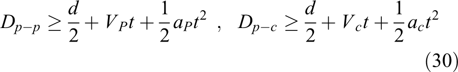
D_{p - p} \geq \frac{d}{2} + V_{P} t + \frac{1}{2} a_{P} t^{2}, D_{p - c} \geq \frac{d}{2} + V_{c} t + \frac{1}{2} a_{c} t^{2}

In equation (30), d is vehicle’s width, V_P is initial walking speed of pedestrian, V_c is initial walking speed of cyclist, a_P is pedestrian’s braking deceleration, and a_c is bicycle’s braking deceleration. Lateral distance is expressed as a function of distance with time.

Simulation

In order to verify the validity and effectiveness of path planning, CarSim and Simulink are simulated to evaluate the performance between basic ant colony algorithm and fusion algorithm method. CPU of simulation platform is Intel core i7-5500U, the RAM is 8.00 GB, the MATLAB version is R2014a, and the CarSim version is 8.1. Figure 17 shows comparisons between basic ant colony algorithm and fusion algorithm method on individual fitness and iteration times of path searching progress.

Figure 17.

(a) Curve of pheromone concentration increment, (b) curve of iteration times under the influence of pheromone concentration, and (c) curve of convergence.

As vividly shown in Figure 17, pheromone concentration increment affected by improved fusion algorithm increases faster than that affected by ant colony algorithm. It reaches to the set threshold ( $τ = 0.6$ ) in initial stage of iteration (near 7 times), however, updated pheromone concentration which is influenced by basic ant colony algorithm reaches to $τ = 0.6$ at 18 iteration times.

Benefit from the dynamic adjustment of pheromone update strategy, efficiency of path searching can be adjusted according to pheromone coefficient volatilization. In a certain range (0.3–0.7), increase of pheromone volatilization coefficient will improve path searching efficiency. Basic ant colony algorithm needs 32 iterations to converge to the optimal path, while improved fusion algorithm needs 14 iterations to achieve optimal path. Table 3 shows comparison of simulation results.

Table 3.

Comparison of simulation results.

Algorithm	Basic ant colony algorithm	Improved fusion algorithm
Length of optimal path (m)	164.247	162.415
Iteration times (s)	32	14
Running time (s)	17.418	5.723

The vehicle system used for simulation in CarSim software is a model of advantage driving assistance system. Variation of vehicle dynamic parameters during typical path planning progress is shown in Figure 18.

Figure 18.

Variation of all vehicle dynamic parameters during typical path planning progress.

As vividly shown in Figure 18, autonomous vehicle perceives the location of front obstacle firstly, slows down the speed from 60 km h⁻¹ to 27.8 km h⁻¹ gradually, steering the wheel if collision cannot be avoided by braking alone. Wheel steering angle changes from 0° to 12.6° yaw rate, vehicle changes from 0° s⁻¹ to 7.2° s⁻¹. All parameters of autonomous vehicle during obstacle avoidance path planning are changed within reasonable range.

Method of comparison will be used to verify the performance of vehicle dynamic under the situation with or without traffic accident risk. Results are shown in Figure 19.

Figure 19.

(a) Performance of vehicle dynamic without traffic accident risk and (b) performance of vehicle dynamic with traffic accident risk.

Figure 19 shows that, under no traffic accident risk scenario, autonomous vehicle accelerates along preplanned path at beginning, slows down gradually due to the effect of repulsion potential field which is formed by front vehicle, and drives at same speed as front vehicle. What’s more, lateral stability of this vehicle is very significant. All parameters of vehicle dynamic fluctuate in a very small range which can be seen in Figure 19(a).

Figure 19(b) shows the performance of vehicle dynamic under existence of traffic accident risk condition. Pedestrains, bicycles which appeared suddenly in front of ego vehicle leads to the change of lateral position when autonomous vehicle driving to target. With start of steering process, lateral acceleration of vehicle changes from −0.423 g to 0.72 g, yaw rate changes from −8.43° s⁻¹ to 10.07° s⁻¹. Sideslip angle of tire changes from −1.16° to 1.02°. Consequently, autonomous vehicle will slightly deviate from the original path; as soon as it passes the pedestrian or bicycle, road potential field leads autonomous vehicle back to planned path. Moreover, speed of autonomous vehicle does not change noticeably in this scenario, as expected. All parameters are changed within reasonable range to meet requirements of steering stability and driving safety during steering process.

Conclusion

In this article, a new fusion algorithm combining ant colony algorithm and improved potential field is introduced. This algorithm generates path based on vehicle dynamics, road structure, traffic regulations, and adhesion coefficient of driving road.

Estimation algorithm for road adhesion coefficient is added to path planning, expect for road structure, vehicle dynamic, and traffic regulations. It’s significant for autonomous vehicle to improve accuracy of road recognition. After simulation and comparative analysis, validity of path planning under low road adhesion coefficient condition was verified.

Virtual potential field which considers different PFs for different obstacles, road structure, and traffic regulations under multi-category objects was establishment. In addition, a reasonable trajectory with less iteration can be planned when joint potential force is added as heuristic information function to fusion algorithm used for path searching process. In other word, blindness, randomness, and stagnation of path searching due to low pheromone concentration at initial stage of path searching progress will be avoided, and efficiency of path search will be improved.

Whether there is no traffic accident risk or existence of traffic accident risk, all parameters of autonomous vehicle in the above two simulations are changed within reasonable range to meet the requirements of driving stability and safety.

Results showed the capability of fusion algorithm in preforming appropriate maneuvers in path planning process. Besides, since vehicle dynamic, traffic regulation, and adhesion coefficient were considered, fusion algorithm used in path planning performs better.

Footnotes

Declaration of conflicting interests

The author(s) declared no potential conflicts of interest with respect to the research, authorship, and/or publication of this article.

Funding

The author(s) disclosed receipt of the following financial support for the research, authorship, and/or publication of this article: This project is supported by the National Natural Science Foundation of China (Grant No. 51775247, 51305167) and Postgraduate Research & Practice Innovation Program of Jiangsu Province (Grant No. KYCX18_2230).

ORCID iD

Yue Wei

References

Editorial Department of China Journal of Highway and Transport. Summary of academic research on automotive engineering in China. China J Highw Transp 2017; 30(6): 1–197.

Karaman

Frazzoli

. Sampling-based optimal motion planning for non-holonomic dynamical system. Int J Robot Res 2011; 30(7): 846–894.

Goerzen

Kong

Mettler

. A survey of motion planning algorithms from the perspective of autonomous UAV guidance. J Intell Robot Syst 2010; 57(1–4): 65.

Dolgov

Thrun

Montemerlo

, et al. Path planning for autonomous vehicles in unknown semi-structured environments. Int J Robot Res 2010; 29(5): 485–501.

Xiu

Chen

. Research on local path planning of driverless vehicle based on improved artificial potential field method. Automot Eng 2013; 35(9): 808–811.

Zhu

. Research on vehicle obstacle avoidance path planning based on improved artificial potential field method. Jiangsu University, China, 2017.

Khajepour

Melek

, et al. Path planning and tracking for vehicle collision avoidance based on model predictive control with multiconstraints. IEEE Trans Veh Technol 2017; 66(2): 952–964.

Wang

. Research on adaptive path planning for vehicle routing problem based on ant colony algorithm. Qingdao University of Science & Technology, China, 2011, pp. 27–40.

Gao

Cheng

Wang

, et al. Object classification using CNN-based fusion of vision and LIDAR in autonomous vehicle environment. IEEE Trans Ind Informat 2018; 14: 4224–4231.

10.

Wang

. Research on millimeter wave radar and machine vision fusion of front vehicle detection. Jilin University, China, 2013, pp. 26–47.

11.

Luo

Yao

Zhang

. A joint calibration method for millimeter wave radar and camera. J Tsinghua Univ 2014; 54(3): 289–293.

12.

. Theory of Automobile. Beijing, China: China Machine Press, 5th edition, 2009, pp. 145–147.

13.

Gao

Gray

Tseng

, et al. A tube-based robust nonlinear predictive control approach to semiautonomous ground vehicles. Veh Syst Dyn 2014; 52(6): 802–823.

14.

Yuan

Zhang

Chen

. Research on identification algorithm of road adhesion coefficient. Automot Eng 2017; 39(11): 1268–1273.

15.

Yang

. A 4WD + 4WS VSC system modeling based on Burckhardt tire model. J of Zhejiang Wanli Uni 2012; 25(3): 67–75.

16.

Khatib

. Real-time obstacle avoidance for manipulators and mobile robots. Int J Robot Res 1986; 5(1): 90–98.

17.

Ren

Cui

. Preview control and steady state error analysis of lane keeping. Automot Eng 2016; 38(2): 191–199.

18.

Yin

Jia

. Fuzzy predictive control for path tracking of autonomous vehicle. J North Univ China 2011; 32(2): 135–139.

19.

Rasekhipour

Khajepour

Chen

, et al. A potential field-based model predictive path-planning controller for autononous road vehicles. IEEE Trans Intell Transp Syst 2017; 18(5): 1255–1269.

20.

Gao

Shi

Xie

, et al. Car-following method based on inverse reinforcement learning for autonomous vehicle decision-making. Int J Adv Robot Syst 2018; 15(6): 1–11.

21.

Gao

Xie

, et al. Hardware and software architecture of intelligent vehicles and road verification in typical traffic scenarios. IET Intell Transp Syst 2018; 13(6): 960–966.

Research on path planning based on new fusion algorithm for autonomous vehicle

Abstract

Keywords

Introduction

Environment perception

Path planning

Vehicle dynamic model

Estimation algorithm for adhesion coefficient

Improved potential field

Path planning

Improvement of transfer probability function

Adjustment of pheromone update strategy

Results

Test scenarios

Simulation

Conclusion

Footnotes

Declaration of conflicting interests

Funding

ORCID iD

References