Sage Journals: Discover world-class research

Abstract

Safe lane changing of the dynamic industrial park and port scenarios with autonomous trucks involves the problem of planning an effective and smooth trajectory. To solve this problem, we propose a new trajectory planning method based on the Dijkstra algorithm, which combines the Dijkstra algorithm with a cost function model and the Bezier curve. The cost function model is established to filter target trajectories to obtain the optimal target trajectory. The third-order Bezier curve is employed to smooth the optimal target trajectory. Road experiments are carried out with an autonomous truck to illustrate the effectiveness and smoothness of the proposed method. Compared with other conventional methods, the improved method can generate a more effective and smoother trajectory in the truck lane change.

Keywords

Autonomous truck trajectory planning Dijkstra algorithm cost functional model Bezier curve

Introduction

Motivation

In recent years, research on autonomous vehicles has entered a period of vigorous development. More and more autonomous vehicles are tested on real urban roads. Some companies even have begun the trial operation of autonomous vehicles. In the passenger car field, Google Waymo has launched the self-driving taxi business in California, USA. In the commercial vehicle field, TuSimple has commercialized the road freight business in Arizona, USA. Autonomous vehicles use their sensing devices to perceive the surrounding environment, make executable safety decisions through the decision-making subsystem, confirm the effectiveness of the behavior, plan its trajectory, and finally complete autonomous driving.

As a research branch of intelligent robots, many technologies of autonomous vehicles are derived from intelligent robots. The trajectory planning of autonomous driving is equivalent to that of intelligent robots in a special scene. The trajectory planning of the intelligent robot is carried out in three-dimensional space, while the trajectory planning of autonomous driving is similar, but limited to a two-dimensional plane. Therefore, the study of trajectory planning for autonomous driving can refer to current studies on the trajectory planning of intelligent robots.^1

–9 The problem of trajectory planning for autonomous driving can be regarded as a time–space curve optimization problem in a two-dimensional plane, and solving the optimization problem means solving the problem of trajectory planning for autonomous driving.

At present, there are various methods that can achieve trajectory planning for autonomous vehicles. The common trajectory planning methods for autonomous vehicles are the Dijkstra algorithm combined with the Bezier curve and the A-star algorithm combined with the Bezier curve. The Dijkstra algorithm combined with the Bezier curve is limited by the amount of calculation of the Dijkstra algorithm, which increases the response time of the vehicle. In practice applications, this method requires a larger computing device to calculate all the candidate target trajectories to obtain an optimal target trajectory. The A-star algorithm combined with the Bezier curve is mainly used for the trajectory planning of passenger cars. However, since the size of the truck is larger than the size of the passenger car, the method of trajectory planning may be different. Therefore, it is not an effective method in the trajectory planning of autonomous trucks. In this article, an improved Dijkstra method is proposed for these problems. The main contribution of this article lies in (1) the proposed method uses a different cost function model and makes it different from previous work in that it is especially suitable for autonomous trucks and (2) the experimental studies to verify the proposed method.

Related work

The autonomous vehicle generates the desired path according to various parameters that are fed as input from the sensors and provides a corresponding control signal to the actuators that drive the vehicle to complete the autonomous driving. The vehicle’s autonomous driving system is mainly divided into three subsystems: the perception subsystem, the decision-making subsystem, and the actuator subsystem, each of which performs different tasks. The perception subsystem is mainly responsible for environmental perception and positioning. The decision-making subsystem mainly completes the motion planning and trajectory planning of the vehicle, and the actuator subsystem is in charge of the execution of the motion command to help the vehicle complete the driving task. Decision-making is an important module for autonomous driving. It determines whether the vehicle can smoothly and accurately complete various driving behaviors. Trajectory planning is a significant research field in the decision-making layer.¹⁰ Trajectory planning mainly implements driving behavior commands through the behavior planning layer to satisfy the movement and dynamic constraints of the vehicle and avoid collisions. The workflow chart of the trajectory planning layer is shown in Figure 1. The blue coating part in Figure 1 is the trajectory planning layer framework. Due to the complexity of the real urban environment, and the non-holonomic vehicle system, it is very difficult to carry out trajectory planning during driving.The trajectory planning layer should generate executable trajectories that correspond to each behavioral result. In fact, trajectory planning is a constrained optimization problem, and the constraints include the vehicle’s current state (i.e. planned and initial state) behavior and target vehicle dynamics, constituting the final trajectory optimization. The trajectory that meets these criteria can be used as the final output trajectory.

Figure 1.

The flowchart of the trajectory planning layer.

In the past decade, autonomous driving technology has been developed as a promising technology. Trajectory planning, as a major challenge of autonomous driving technology,^10,11 has also made significant progress. The algorithms related to trajectory planning can be divided into four categories: interpolating-curve-based, graph-search-based, sampling-based, and numerical-optimization-based.^12,13 Graph-search-based algorithm extends from algorithms for path planning; the most common graph-search-based algorithms for trajectory planning are Dijkstra,¹⁴ A-star,¹⁵ and state lattice.¹⁶ The Dijkstra algorithm is suitable for finding the shortest path in both structured and unstructured environments. Its result is continuous but not smooth, and it is computationally intensive. The A-star algorithm reduces the computational cost. The output result is continuous but not smooth. The state lattice algorithm can process multidimensional computation and is suitable for the dynamic environment and local planning, but it takes long time to compute. The most common sampling-based algorithm for trajectory planning is rapidly exploring random tree (RRT).¹⁷ It can be solved quickly in a high-dimensional system with convergence and completeness. Its result is continuous but not smooth. The most common interpolating-curve-based algorithms are Clothoid curves,¹⁸ polynomial spirals,¹⁹ Bezier curves,²⁰ and spline curves.²¹ The Clothoid curve algorithm is suitable for local planning. It is easy to implement on high-speed and structured roads, but the integration can be time-consuming. The curvature is continuous but not smooth, depending on waypoints. The polynomial spirals algorithm works without heavy calculation, and its curvature is continuous. But the curvature is more than four orders, of which the key parameters are also not easy to obtain. Sharing similar advantages as the polynomial spirals algorithm when the curve order is not large, the Bezier curve algorithm has lower ductility when the curve order is increased, resulting in the massive calculation. The spline curves algorithm also has worked without much calculation and generates smooth curves, but its output curve may not be the optimal one. The most common numerical-optimization-based algorithm is function optimization algorithms.²² In the case of considering various constraints, function optimization is easy to implement but has high computational cost and relies heavily on waypoints.

Autonomous truck

Firstly, we introduce an autonomous truck shown in Figure 2, which was modified based on ordinary trucks. This truck’s autonomous system consists of an autonomous driving control unit (ADCU), a wire control chassis of the truck, a high-precision inertial measurement unit (IMU), and sensors group, including 16-line LiDARs, a single-line LiDAR, ultrasonic radars, a front-view camera, and a side-view camera. The truck’s dimension is $7000 \times 2200 \times 4000 {mm}^{3}$ .

Figure 2.

Autonomous truck.

As is shown in Figure 3, the driving system of the truck is mainly composed of the environment perception subsystem, the decision-making subsystem, and the actuator subsystem.The perception subsystem is mainly composed of 16-line LiDARs, a single-line LiDAR, ultrasonic radars, a front-view camera, a side-view camera, and high-precision IMUs. The front-view camera is used for visual target recognition. The side-view camera is used for target recognition, positioning, and parking assist. The ultrasonic radars are used to detect obstacles on the road that may cause a scratch on the vehicle chassis. The high-precision IMU is used to acquire the path planning information and the precise positioning information of the vehicle. The single-line LiDAR is used for obstacle measurement and collision avoidance. High-definition map (HD map) is used for providing the surrounding environment information, road information, intersection information, and making the path plan for the truck.

Figure 3.

Autonomous driving system architecture.

The 16-line LiDARs are used for simultaneous localization and mapping (SLAM) positioning and obstacle detection. When the global positioning system signal is weak, or the vehicle is in the tunnel, the 16-line LiDARs are used for SLAM positioning, and the visualization method is combined to improve the positioning accuracy of SLAM. Figure 3 shows an example of the SLAM-visual combined positioning solution. In Figure 4(a), the yellow marks represent the vehicle’s global path. In Figure 4(b), we can see the partial path is composed of many yellow feature points by which the vehicle is positioned. Figure 4(c) shows a case in which the side-view camera helps improve the positioning accuracy. When target feature points are captured, they will be compared with the key feature points stored in the device to obtain an accurate position.

Figure 4.

Accurate combination positioning solution: (a) global path, (b) partial path, (c) camera key feature points comparison.

All sensor information is output to the ADCU, and the obstacle information and vehicle position information are obtained through the fusion algorithm. Then the information is output to the decision-making subsystem for truck behavior planning and trajectory planning. According to the output of the behavior planning and trajectory planning, the control signals are transmitted to the actuator subsystem for vehicle control.

Trajectory planning algorithm

Trajectory planning is executed by the decision planning layer to drive the behavior instructions output. Trajectory planning generates a series of trajectory curves from the current state to the next goal state. In the real urban environment, the trajectories need to satisfy the movement and dynamic constraints of the vehicle to avoid collision with obstacles.

Trajectory generation model

In the trajectory planning of autonomous trucks, the graph-based search method is to search the optimal path (state sequence) between the current state of the truck and the next goal state in the graph-based state space.

In this article, the problem of lane-level path planning for trucks on HD maps is abstracted into a shortest path search problem on directed weighted maps. When the HD map of the lane level is obtained, the “scatter points” are carried out in a certain range of lanes, representing the possible driving position of the vehicle.

The trajectory of an autonomous vehicle can be regarded as a set of actions from the initial state X ₀ to the goal state X_T

X_{0} = [x_{0} . y_{0}, k_{0}]

X_{T} = [x_{T} . y_{T}, k_{T}]

Among them, $(x, y)$ represents the vehicle’s position in a two-dimensional coordinate system and k represents the curvature of the vehicle’s trajectory. The transformational relation among curvature k, turning radius r, wheelbase L, and front-wheel angle α is expressed as follows²³

k = 1 / r = tan α / L

As is shown in Figure 5, the candidate trajectory is generated by connecting the sampling points, and the planning area is between the red lines.

Figure 5.

Candidate trajectory.

Cost function based on vehicle motion constraints

In terms of trajectory planning of autonomous vehicles, the most common techniques are sampling graph search methods, such as the Dijkstra algorithm, A-star algorithm, and its variants. An improved Dijkstra algorithm is proposed in this article, combining the original Dijkstra algorithm (introduced in Appendix) and the cost function. The cost function model for trajectory planning is established as truck motion constraint exists. Considering the vehicle’s steering ability when randomly distributing sampling points, not only should the shortest Euclidean distance $Dist (p_{i}, p_{j})$ be considered but also the smoothness of the trajectory $Head (p_{i}, p_{j})$ is expected to be as small as possible. In addition, considering the initial state constraints of the vehicle, the tangent vector of the starting point and the second sampling point should to be horizontal, so the $Head (p_{0}, p_{1})$ should be 0. Based on the above analysis, a more reasonable cost function (see equations (4) to (6)) which is in line with the practical application of autonomous vehicles has been chosen in this article. Figure 6 shows the nodes of the cost function

Cost (p_{i}, p_{j}) = K_{1} Dist (p_{i}, p_{j}) + K_{2} Head (p_{i}, p_{j})

Dist (p_{i}, p_{j}) = Norm (\sqrt{{(x_{i} - x_{j})}^{2} + {(y_{i} - y_{j})}^{2}})

Head (p_{i}, p_{j}) = Norm (θ_{i j})

Figure 6.

The nodes of the cost function.

Among them, K ₁ and K ₂ are weights of distance and angle difference, respectively, which can be set according to the actual situation, and $(x_{i}, y_{i})$ and $(x_{j}, y_{j})$ are coordinates of p_i and p_j , respectively. Captured by sensors with two different forms, the distance and angle data need to be normalized to unify them under the same reference. In this article, an effective and simple deviation normalization approach is adopted to deal with these two variables (see equations (7) and (8)). Among them, $d_{max}$ and $d_{min}$ represent the largest node distance and the smallest node distance, respectively, and $θ_{max}$ and $θ_{min}$ represent the largest angle and the smallest angle between nodes, respectively. Norm function calculates the normalized distance d and angle θ, respectively

Norm (d) = (d - d_{min}) / (d_{max} - d_{min})

Norm (θ) = (θ - θ_{min}) / (θ_{max} - θ_{min})

According to the Dijkstra algorithm, all the nodes are checked successively, with their neighbors added to the list of nodes to be checked. The algorithm stops when it reaches the goal node. Figure 7 shows the flowchart of the proposed algorithm.

Figure 7.

The flowchart of the algorithm.

Firstly, the data list of sampling points is read. The number of sampling points in the list is n. The starting point and the ending point are marked, respectively. And the number of sampled points is denoted by $num (1 \leq num \leq n)$ .

Then, start from the starting point to find the unmarked point with the lowest cost in the sampling point list to be the next point. And the initial cost is marked as 0. Next, examine all the remaining unsampled nodes in turn and add their adjacent points to the list of points to be checked.

After traversing from the start point to each point, if the cost of point num is smaller than the current minimum, update the minimum, $num = num + 1$ .

Repeat the above process until reaching the end point.

Smooth trajectory curve

Bezier curve is used to smooth the trajectory connecting the starting and ending points. The Bezier curve only needs a few control points to generate a more complex smooth curve. This method can ensure the clear and simple relationship between the input control points and the generated curve, and the shape and order of the curve can be easily changed.^24

–28 Given the position vector of n + 1 point in space, the coordinate of each point on the Bezier reference curve can be obtained by the following formula

T (t) = \sum_{i = 0}^{n} P_{k} B_{k, n} (t) t \in [0, 1]

Among them, P_i represents the control point, $T (t)$ represents trajectory function with time, and t is the time proportional coefficient, n is the order of curve, and $B_{k - n} (t)$ is the Bernstein basis function

\begin{matrix} B_{k, n} (t) = C_{n}^{i} t^{i} {(1 - t)}^{n - i} \\ = \frac{n!}{i! (n - i)!} t^{i} {(1 - t)}^{n - i} \end{matrix}

Bezier curve has characteristics of the convex hull, symmetry, geometric invariance, quasi-locality, and so on. It guarantees the smoothness, continuity, and controllability of the generated curve. In the third-order Bezier curve,²⁹ point P ₀ is used as the center coordinate of the goal vehicle, points P ₁ and P ₂ in the middle of the trajectory curve are used as the control points, and the goal point is represented by point P ₃. P ₀, P ₁, P ₂, and P ₃ points are illustrated on an example trajectory curve as shown in Figure 8.

Figure 8.

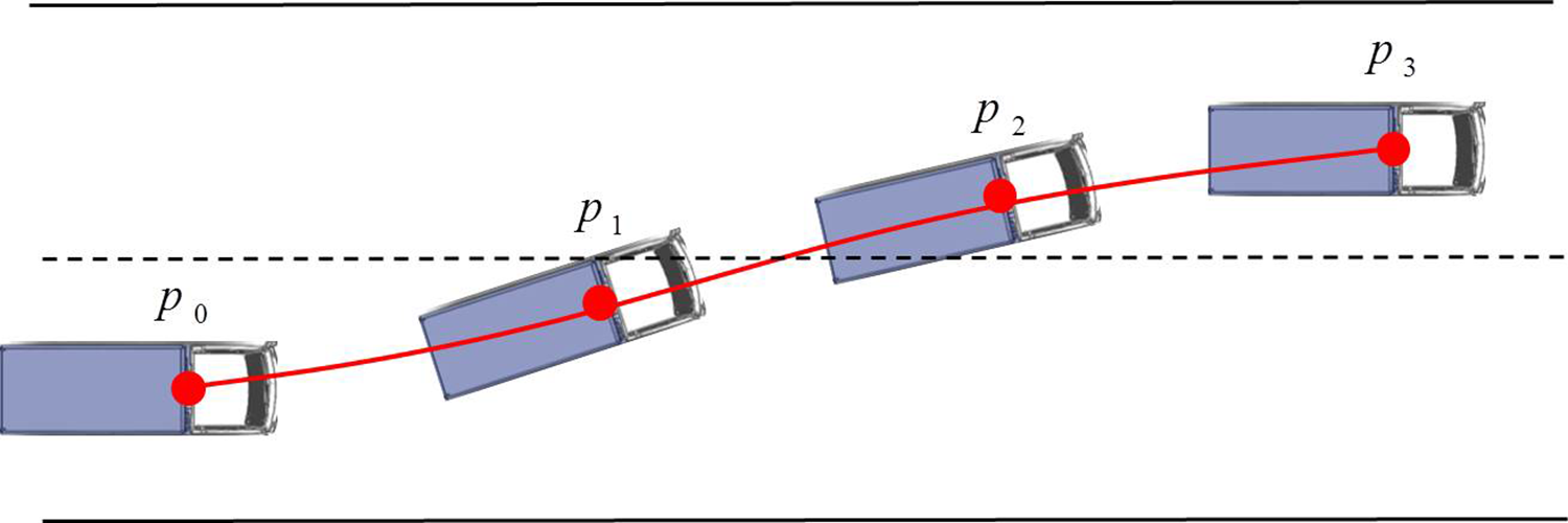
Illustration of control points.

Because changing direction in situ can damage the vehicle’s tires, it is necessary to let the vehicle follow a smooth trajectory. At the same time, when changing lanes or turning, it is necessary to follow traffic rules and go along a proper road when planning the trajectory. This article plans the vehicle’s trajectory points as mentioned earlier. The third-order Bezier curve determined by the four control points can be obtained by the following formula

\begin{matrix} T (t) = {(1 - t)}^{3} P_{0} + 3 t {(1 - t)}^{2} P_{1} \\ + 3 t^{2} (1 - t) P_{2} + t^{3} P_{3} \end{matrix}

T (t) = [\begin{matrix} t^{3} & t^{2} & t & 1 \end{matrix}] [\begin{matrix} - 1 & 3 & - 3 & 1 \\ 3 & - 6 & 3 & 0 \\ - 3 & 3 & 0 & 0 \\ 1 & 0 & 0 & 0 \end{matrix}] [\begin{matrix} P_{0} \\ P_{1} \\ P_{2} \\ P_{3} \end{matrix}]

Road experiments

Road experiments were carried out in a port to evaluate the performance of the proposed algorithm. In the experiment, the road is a four-lane dual carriageway with the width of 3.5 m. The horizontal distance between the start point and the end point is set to be 300 m. In this section, we present the results of the experiment in the lane change scene as shown in Figure 9.

Figure 9.

Lane change scene.

This lane change scene is a situation when the truck encounters a static vehicle in front of it during driving, and the truck needs to change lane to avoid the collision. The results of the experiment show that the truck smoothly changes the lane and avoids the obstacle and collision. The results of the experiment include the heading angle, the yaw, and the trajectory curvature of the truck. They are used to evaluate the motion control performance and comfortness of the vehicle.

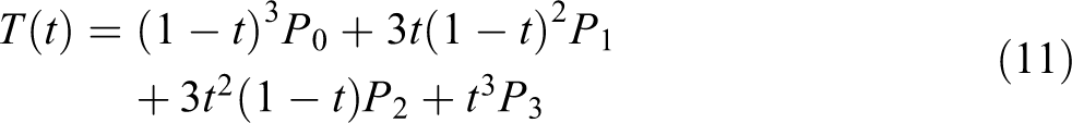
Since Figure 9 cannot show the lane change process of the truck, we use a schematic diagram to indicate the lane change process of the truck. The schematic diagram of truck lane change is shown in Figure 10.

Figure 10.

Truck lane change.

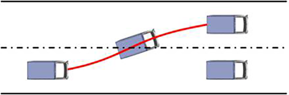
The trajectory curves

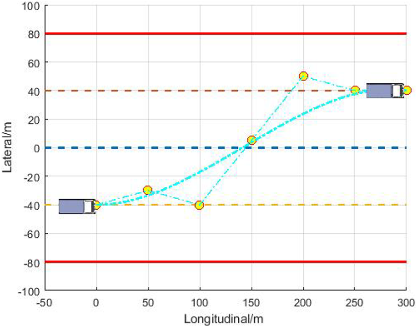
After the experiment, the trajectory curve generated by the truck is analyzed. The trajectory of the candidate sampling points is generated according to the Dijkstra algorithm with the cost function model, the Bezier curve, and the constraints of the vehicle’s direction. The heading angle of the truck at the starting point and the ending point is one of the constraints, which should be horizontal and suitable for the scene of the lane change. Through the improved Dijkstra method, the trajectory generated by the vehicle is shown in Figure 11. The polyline in the figure is generated by the Dijkstra algorithm combined with the cost function model, and the smooth curve is obtained by smoothing the polyline through the Bezier curve.

Figure 11.

The trajectory curve of the improved Dijkstra method.

The trajectory generated by the Dijkstra method is shown in Figure 12. The target trajectory shown by the polyline in the figure is generated using the Dijkstra algorithm, and then the smooth curve in the figure is obtained by smoothing the polyline with the Bezier curve.

Figure 12.

The trajectory curve of the Dijkstra method.

Similarly, the trajectory planning of the A-star method is considered for better comparison. The A-star algorithm is based on the combination of Dijkstra algorithm and a cost function model, like the improved Dijkstra algorithm. As is shown in Figure 13, the polyline represents the trajectory generated by the A-star algorithm, and the smooth curve represents the trajectory generated by the Bezier curve.

Figure 13.

The trajectory curves of the A-star method.

The results of the experiment

The trajectory curves of these three methods are shown in Figure 14. The trajectory generated by the improved Dijkstra method proposed in this article is different from that generated by the A-star method and the original Dijkstra method. Since it is not easy to obtain much information through the trajectory curves, the quantitative experiment results are also necessary to be compared.

Figure 14.

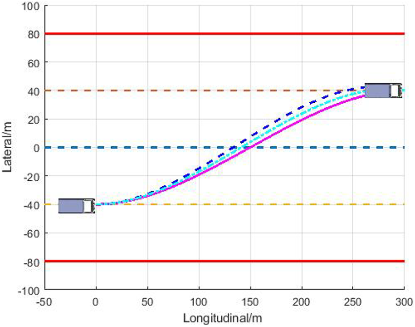
The comparison of three methods (purple curve: improved Dijkstra method, blue curve: Dijkstra method, and cyan curve: A-star method).

The heading angle represents the direction of the vehicle. The heading angle of the starting point and the ending point of the vehicle should be the same. The yaw value represents the rate of deflection change around the vertical axis. It has to be noticed that if the yaw value of the truck changes too fast, the sideslip or tail-flick will occur. As is shown in Figure 15, the heading angles and the yaw values of the three methods are calculated, respectively.

Figure 15.

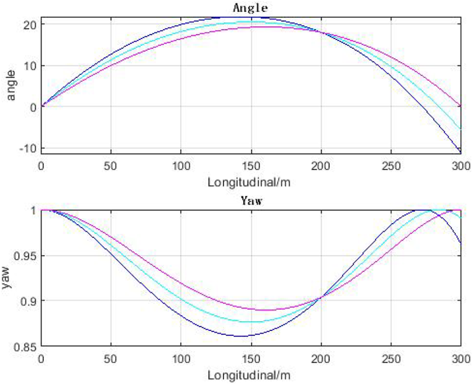
The (a) heading angle and the (b) yaw value of the truck trajectory with three methods (purple curve: improved Dijkstra method, blue curve: Dijkstra method, and cyan curve: A-star method).

The purple curve represents the improved Dijkstra method. The vehicle heading angle increases from $0^{\circ}$ to ${19.3785}^{\circ}$ , then decreases to $0^{\circ}$ . The starting heading angle is the same as the ending heading angle. The minimum yaw value is $0.8899 rad s^{- 1}$ , and the maximum yaw is $1 rad s^{- 1}$ .

The blue curve indicates the Dijkstra method. The vehicle heading angle increases from $0^{\circ}$ to ${21.8612}^{\circ}$ , decreases to $0^{\circ}$ before the vehicle arrives at the end point, and then overshoots to $- {11.3099}^{\circ}$ . The starting heading angle is different from the ending heading angle, which does not meet the requirement of the lane change scene. The minimum yaw value is $0.8613 rad s^{- 1}$ , and the maximum yaw is $1 rad s^{- 1}$ .

Similarly, the cyan curve represents the A-star method. The vehicle heading angle increases from $0^{\circ}$ to ${20.556}^{\circ}$ , and then also overshoots to $- {5.7106}^{\circ}$ . The heading angle of the starting point and the ending point does not meet the actual vehicle orientation. The minimum yaw value is $0.8767 rad s^{- 1}$ , and the maximum yaw is $1 rad s^{- 1}$ .To ensure the smoothness of the driving trajectory, it is necessary to judge the curvature of the trajectory. The smaller the curvature of the planning trajectory curve, the larger the lane radius and the better the ride comfortness. Otherwise, if the curvature of the planning trajectory curve is too large, the vehicle will roll over, which has a great impact on safety.

Furthermore, the curvature of the trajectory at each step should be considered comprehensively. The curvature k at point $(x, y)$ is

k (t) = \frac{x^{'} (t) {y^{'}}^{'} (t) - {x^{'}}^{'} (t) y^{'} (t)}{{(x^{'} {(t)}^{2} + y^{'} {(t)}^{2})}^{3 / 2}}

As is shown in Figure 16, the curvature of the trajectory is continuous. Among them, the curvature variation range of the improved Dijkstra method is $[- 0.0053, 0.0053] m^{- 1}$ , the curvature variation range of the Dijkstra method is $[- 0.0075, 0.0067] m^{- 1}$ , and the curvature variation range of the A-star method is $[- 0.0066, 0.0060] m^{- 1}$ .

Figure 16.

The curvature of the truck trajectory with three methods (purple curve: improved Dijkstra method, blue curve: Dijkstra method, and cyan curve: A-star method).

Comparisons are presented in Table 1 to show the performance parameters of the three methods. It can be seen that the maximum heading angle of the improved Dijkstra method is ${19.3785}^{\circ}$ , and it is smaller than the other two methods. The variation range of heading angle is smaller; the deviation of the vehicle is smaller, which is more conducive to the motion control of the vehicle. In addition, it meets the same requirements as the starting point and the ending point. The minimum yaw value of the improved Dijkstra method is larger than the other two methods, the yaw value decreases from $1 rad s^{- 1}$ to $0.8899 rad s^{- 1}$ and then returns to $1 rad s^{- 1}$ . The variation range of the yaw value is smaller, the impact on lateral vehicle control is smaller, and the comfortness is better. Similarly, the curvature of the improved Dijkstra method is the smallest and less than the limit of $0.08 m^{- 1}$ . Therefore, the vehicle motion control performance of this method is more effective.

Table 1.

The parameters of three methods.

Method	Maximum angle (°)	Minimum angle (°)
Improved-D	0	19.3785
Dijkstra	−11.3099	21.8612
A-star	−5.7106	20.556
Method	Maximum yaw value (rad s⁻¹)	Minimum yaw value (rad s⁻¹)
Improved-D	1	0.8899
Dijkstra	1	0.8613
A-star	1	0.8767
Method	Maximum curvature (m⁻¹)	Minimum curvature (m⁻¹)
Improved-D	0.0053	−0.0053
Dijkstra	0.0067	−0.0075
A-star	0.0060	−0.0066

Through comparisons of the results, it can be concluded that the improved Dijkstra method in this article is more suitable for the current trajectory planning of autonomous trucks than Dijkstra and A-star methods. It can generate an effective and smooth trajectory to help the truck change lane.

Conclusions and future work

This article proposes a new trajectory generation method, which combines the Dijkstra algorithm, the cost function model, and the Bezier curve. The trajectory planning model is used for a real truck experiment. The results of the road experiment demonstrate that the trajectory planning method in this article can realize effective and smooth vehicle lane changing and some basic autonomous functions in simple industrial parks and ports.

However, with the trajectory in complex scenes being too complicated, the real-time performance of this algorithm cannot meet the requirements of the complex road. Therefore, in future work, we will delve into the real-time strategy of RRT and study how to integrate RRT real-time strategy into the Dijkstra algorithm or cost function model. In addition, we hope that the application of the fifth-order Bezier curve into the trajectory algorithm can enable vehicles to be more effective and smoother when changing lanes, which is more similar to the driving method of humans. In view of the problem that the amount of computation caused by the fifth-order Bezier curve is greatly improved, we consider improving the computing capacity of the controller or optimize the Bezier curve.

Footnotes

Authors’ note

FZ and RX are co-first authors.

Declaration of conflicting interests

The author(s) declared no potential conflicts of interest with respect to the research, authorship, and/or publication of this article.

Funding

The author(s) disclosed receipt of the following financial support for the research, authorship, and/or publication of this article: This research was supported by the China Scholarship Council (201706160029).

ORCID iD

Xinxing Chen

Appendix

The Dijkstra algorithm, a typical single-source shortest path algorithm, is used to calculate the shortest path from one node to all other nodes in a weighted graph. The Dijkstra algorithm uses a greedy strategy, declaring an array “dis” to hold the shortest distance from the source point s to each vertex and a set of vertices T from which the shortest path to s have been found.

Initially, there is only one vertex in T and the source point s. If there is a directly reachable edge $(s, m)$ for the vertex s to vertex m, then dis[m] is set to the length of edge $(s, m)$ , $w (s, m)$ . Otherwise, dis[m] is set to infinity.

Then, add the vertex m with the minimum dis[m] to T. After that, check if the newly added vertex can be directly reached by other vertices and see if the path length through the vertex to other points is shorter than the direct arrival of the source point. If so, replace the corresponding value in “dis” with the shortest sum of length.

Repeat the above process until T contains all the vertices of the graph. The array “dis” is the length of the shortest path from the source node s to any other nodes.

References

Yin

Wang

. A machine learning based energy efficient trajectory planning approach for industrial robots. Procedia CIRP 2019; 81: 429–434.

Kim

Croft

. Online near time-optimal trajectory planning for industrial robots. Robot Comput-Integr Manuf 2019; 58: 158–171.

Fang

Liu

, et al. Smooth and time-optimal s-curve trajectory planning for automated robots and machines. Mech Mach Theory 2019; 137: 127–153.

Raj

Thakur

. Dynamically feasible trajectory planning for anguilliform-inspired robots in the presence of steady ambient flow. Robot Auton Syst 2019; 118: 144–158.

Wang

Huang

, et al. Smooth point-to-point trajectory planning for industrial robots with kinematical constraints based on high-order polynomial curve. Mech Mach Theory 2019; 139: 284–293.

Sathiya

Chinnadurai

. Evolutionary algorithms-based multi-objective optimal mobile robot trajectory planning. Robotica 2019; 37(8): 1363–1382.

Huang

Zhang

, et al. High-order disturbance observer based sliding mode control for mobile wheeled inverted pendulum systems. IEEE Trans Ind Electron 2019; 67: 2030–2041.

Huang

Cao

Xiong

, et al. An echo state Gaussian process-based nonlinear model predictive control for pneumatic muscle actuators. IEEE Trans Autom Sci Eng 2018; 16: 1071–1084.

Chen

Huang

. Combining particle filter algorithm with bio-inspired anemotaxis behavior: a smoke plume tracking method and its robotic experiment validation. Measurement 2020; 154: 107482.

10.

Badue

Guidolini

Carneiro

, et al. Self-driving cars: a survey. arXiv preprint arXiv:190104407, 2019.

11.

Werling

Ziegler

Kammel

, et al. Optimal trajectory generation for dynamic street scenarios in a Frenet frame. In: 2010 IEEE international conference on robotics and automation, Anchorage, AK, USA, 3–7 May 2010, pp. 987–993. Piscataway, New Jersey, US: IEEE.

12.

González

Pérez

Milanés

, et al. A review of motion planning techniques for automated vehicles. IEEE Trans Intell Transp Syst 2015; 17(4): 1135–1145.

13.

Paden

Čáp

Yong

, et al. A survey of motion planning and control techniques for self-driving urban vehicles. IEEE Trans Intell Veh 2016; 1(1): 33–55.

14.

McKeever

SD.

Path planning for an autonomous vehicle. Technical report, Massachusetts Institute of Technology, Cambridge, 2000.

15.

Papadatos

Research on motion planning of autonomous mobile robot. Technical report, Naval Postgraduate School, Monterey, CA, 1996.

16.

Pivtoraiko

Knepper

Kelly

. Differentially constrained mobile robot motion planning in state lattices. J Field Robot 2009; 26(3): 308–333.

17.

LaValle

Kuffner

Jr . Randomized kinodynamic planning. Int J Robot Res 2001; 20(5): 378–400.

18.

Broggi

Medici

Zani

, et al. Autonomous vehicles control in the VisLab intercontinental autonomous challenge. Annu Rev Control 2012; 36(1): 161–171.

19.

McNaughton

Urmson

Dolan

, et al. Motion planning for autonomous driving with a conformal spatiotemporal lattice. In: 2011 IEEE international conference on robotics and automation, Shanghai, China, 9–13 May 2011, pp. 4889–4895. Piscataway, New Jersey, US: IEEE.

20.

Zhao

Chen

Mei

, et al. Dynamic motion planning for autonomous vehicle in unknown environments. In: 2011 IEEE intelligent vehicles symposium (IV), Baden-Baden, Germany, 5–9 June 2011, pp. 284–289. IEEE.

21.

Wang

Ganjineh

Rojas

. Action annotated trajectory generation for autonomous maneuvers on structured road networks. In: The fifth international conference on automation, robotics and applications, Wellington, New Zealand, 6–8 December 2011, pp. 67–72. IEEE.

22.

Ziegler

Bender

Dang

, et al. Trajectory planning for Bertha—a local, continuous method. In: 2014 IEEE intelligent vehicles symposium proceedings, Dearborn, MI, USA, 8–11 June 2014, pp. 450–457. Piscataway, New Jersey, US: IEEE.

23.

Kelly

Stentz

. Rough terrain autonomous mobility—Part 1: a theoretical analysis of requirements. Auton Robot 1998; 5(2): 129–161.

24.

Howard

Kelly

. Optimal rough terrain trajectory generation for wheeled mobile robots. Int J Robot Res 2007; 26(2): 141–166.

25.

Howard

Pivtoraiko

Knepper

, et al. Model-predictive motion planning: several key developments for autonomous mobile robots. IEEE Robot Autom Mag 2014; 21(1): 64–73.

26.

Ferguson

Howard

Likhachev

. Motion planning in urban environments: Part II. In: 2008 IEEE/RSJ international conference on intelligent robots and systems, Nice, France, 22–26 September 2008, pp. 1070–1076. Piscataway, New Jersey, US: IEEE.

27.

Gómez-Bravo

Cuesta

Ollero

, et al.

Continuous curvature path generation based on

β

-spline curves for parking manoeuvres. Robot Auton Syst 2008; 56(4): 360–372.

28.

Xiao

. On-line planning of nonholonomic trajectories in crowded and geometrically unknown environments. In: 2009 IEEE international conference on robotics and automation, Kobe, Japan, 12–17 May 2009, pp. 3230–3236. Piscataway, New Jersey, US: IEEE.

29.

Zarzycki

. Applied geometry for computer graphics and CAD (2nd edn.), by Duncan Marsh. Pp. 350. £18.95. 2005. ISBN 1 85233 801 6 (Springer Verlag). Math Gaz 2007; 91(520): 183.

An optimal trajectory planning algorithm for autonomous trucks: Architecture,algorithm,and experiment

Abstract

Keywords

Introduction

Motivation

Related work

Autonomous truck

Trajectory planning algorithm

Trajectory generation model

Cost function based on vehicle motion constraints

Smooth trajectory curve

Road experiments

The trajectory curves

The results of the experiment

Conclusions and future work

Footnotes

Authors’ note

Declaration of conflicting interests

Funding

ORCID iD

Appendix

References