Sage Journals: Discover world-class research

Abstract

Lowering joint torques of a robotic manipulator enables lowering the energy it uses as well as increase in the longevity of the robotic manipulator. This article proposes the use of evolutionary computation algorithms for optimizing the paths of the robotic manipulator with the goal of lowering the joint torques. The robotic manipulator used for optimization is modelled after a realistic six-degree-of-freedom robotic manipulator. Two cases are observed and these are a single robotic manipulator carrying a weight in a point-to-point trajectory and two robotic manipulators cooperating and moving the same weight along a calculated point-to-point trajectory. The article describes the process used for determining the kinematic properties using Denavit–Hartenberg method and the dynamic equations of the robotic manipulator using Lagrange–Euler and Newton–Euler algorithms. Then, the description of used artificial intelligence optimization algorithms is given – genetic algorithm using random and average recombination, simulated annealing using linear and geometric cooling strategy and differential evolution. The methods are compared and the results show that the genetic algorithm provides best results in regard to torque minimization, with differential evolution also providing comparatively good results and simulated annealing giving the comparatively weakest results while providing smoother torque curves.

Keywords

Artificial intelligence cooperating robotic manipulators differential evolution genetic algorithm robot trajectory planning simulated annealing

Introduction

To achieve movement, the torque of robot manipulators actuator (e.g. an electrical motor) needs to be higher than the inertial torsion of the joint the actuator is moving.^1,2 The movement requires use of energy directly proportional to the actuator torque. Successfully minimizing the actuator torque, which is dependent on the joint trajectory, will mean that the movement of the robotic manipulator requires less energy, as well as prolong the work life of the robotic manipulator.³

It is possible to define the problem of joint torque optimization in a way that makes it possible to use artificial intelligence (AI) methods, namely the evolutionary computing optimization methods, in an attempt to achieve the lower amounts of actuator torque.^4
–6

Related work

Garg and Kumar⁷ show that optimization of robot manipulator paths in regard to joint torque is possible using a genetic algorithm (GA) in the case of simple robotic manipulators with two degrees of freedom (DOFs), and the authors propose that similar method can be used for a more complex robotic manipulators. Kazem et al.⁴ show the application of a GA on a three-link (redundant) robot arm for point-to-point planning. The paper demonstrated that the GA is an effective method of optimization in that case, capable of achieving multi-objective optimization. Albert et al.⁵ have applied GA to optimize joint angles of a three-link planar manipulator system in regard to path control and accuracy in a point-to-point pick-and-place situation. The paper concludes that GA is applicable when dealing with complex path control – giving improved search speed and approximate solution. Sharma et al.³ attempt to optimize a point-to-point path, interpolated with a fourth-order polynomial, in regard to energy consumed by the robotic manipulator and travelling time with upper limit on the torque. Furthermore, the paper compares the results of a GA with a geometric approach to path planning. The results show a drop in energy consumed when using the path planning with a GA. Wei et al.⁸ show the usage of evolutionary algorithms for the development of collective behaviours, specifically task allocation. Authors propose a two-step scheme for task partitioning and allocation to overcome problems presented by the bootstrapping and deception problems. The results obtained by authors show that the proposed approach leads to better performance in comparison with conventional evolutionary robotics approach. Abu-Dakka et al.⁹ evaluate the efficiency of the time and trajectory smoothness optimization by a multiple population GA using analysis of variance test. Authors conclude that the approach of using a multiple population GA is valid and produces results quickly. Larsen et al.¹⁰ show the application of evolutionary algorithms and rapidly exploring random trees (RRT) with various parameters on a robot system with KUKA KR210 and KUKA R3100 robots on a common axis to calculate collision-free paths. The results show superior results when using evolutionary algorithms in comparison with sampling methods, as well as concluding that the results gained using GA are superior to ones gained with RRT. Wei et al.¹¹ use deep Q-learning AI algorithm to develop end-to-end control policies for robotic swarms. It is shown that use of such techniques enables development of control policies using fewer computation resources, especially in cases with large solution spaces. El Haiek et al.¹² show the trajectory planning of a three-DOF spherical robot with evolutionary algorithms in regard to the minimization of travel time and joint travelling distance. The path is point-to-point and interpolated using polynomial interpolation. Based on the results, by using GA the robot can successfully find an optimal, collision-free, trajectory while minimizing the time and the length of the trajectory.

This article observes the usage of three different algorithms

GA (in two different configurations) which is an algorithm based on natural evolution,^13,14

simulated annealing (SA) (in two different configurations) which is an algorithm based on the metal annealing process^15,16 and

differential evolution (DE), an algorithm inspired by the differential equations.^17,18

The above algorithms are heuristic space search algorithm, designed to search the solution space in an attempt to find the optimal solution. Unlike the deterministic methods, like an extensive search of the solution space, the algorithms used do not guarantee the solution to be the optimal solution, but they often provide good solutions significantly faster in comparison with deterministic methods.^19,20 This article is based on research done in ‘Optimization techniques applied to multiple manipulators for path planning and torque minimization’ by Garg and Kumar,⁷ and attempts to apply the modified techniques on to a more complex case – using a robotic manipulator with six DOFs, as opposed to a robotic manipulator with two DOFs.

Hypothesis

To summarize the novelty of this article, the idea is to investigate

the possibility of evolutionary computing algorithms implementation for optimization of robot manipulator trajectory with respect to minimization of joint torques in cases of complex robotic manipulators and

performance comparison of multiple AI algorithms on solving trajectory planning of complex robot manipulators with minimization of joint torques.

This article compares the results and execution times of aforementioned algorithms and their configurations in two cases – a single robotic manipulator and two cooperating robotic manipulators, both for point-to-point path planning.

Research methodology

In this section, the methodology of the research article will be presented. First, the cases studied in this article will be described, followed with the description of algorithms used to calculate the kinematic and dynamic robotic manipulator equations, followed by the description of algorithms used for optimization.

Cases

This article observes two cases: a single robot manipulator with six DOFs (Figure 1) and two such manipulators working cooperatively by following the same path (Figure 2). Cooperating robotic manipulators are often used in industrial applications.^10,21 In both cases, the method is validated using ABB IRB 120 robotic manipulator. In observed cases, robotic manipulators are transporting a prismatic shaped object with weight of 2 kg along the calculated path.

Figure 1.

Case 1: single robotic manipulator.

Figure 2.

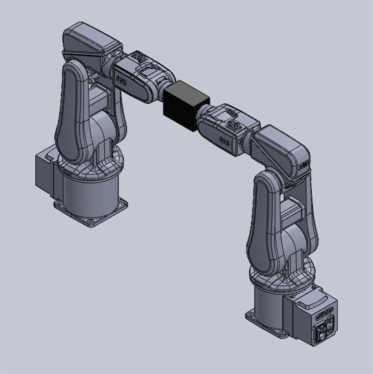
Case 2: two cooperating robotic manipulators.

For path planning, all joints of robotic manipulators start the movement in a position of 0 radian, and finish the movement in 1 radian. The robotic manipulators are stationary at the beginning and the end of the movement making their starting linear and angular velocities as well as the linear and angular accelerations equal zero.^7,22

Robot manipulator dynamics

To determine the dynamic equations, two different algorithms are used – Lagrange–Euler (L-E) and Newton–Euler (N-E). Both algorithms should produce the same results and can be used to check the validity of the calculated results.^23
–25 First step in determining the dynamics of the robotic manipulators is calculating the kinematic matrix. This is also needed for determining the inverse kinematic equations which are necessary for determining the path of the second robotic manipulator in the case with two cooperating robotic manipulators.²⁶

Kinematics

Kinematics are determined using the Denavit–Hartenberg (D-H) method. The D-H method sets the orthonormal coordinate systems in each joint of the robotic manipulator, in such way that axis z^k (where k is a counter determining the joint) matches the axis of movement of the joint k.²⁷ Once all the coordinate systems are positioned, the parameters $θ_{k}$ , d_k , a_k and $α_{k}$ are determined and they are placed in the homogeneous transformation matrix for the joint^28
–30

T_{k - 1}^{k} = [\begin{array}{l} C_{Θ_{k}} & - C_{α_{k}} S_{Θ_{k}} & S_{α_{k}} S_{Θ_{k}} & a_{k} C_{Θ_{k}} \\ S_{Θ_{k}} & C_{α_{k}} C_{Θ_{k}} & - S_{α_{k}} C_{Θ_{k}} & a_{k} S_{Θ_{k}} \\ 0 & S_{α_{k}} & C_{α_{k}} & d_{k} \\ 0 & 0 & 0 & 1 \end{array}]

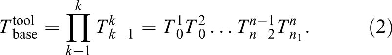
Because of the size of the equations, the shortened trigonometric format is used. When using this format, the trigonometric functions are written using only the first letter of their name, so sine is written as S and cosine as C. In addition, the arguments of the functions are written as indexes – so $sin (α_{1})$ becomes $S_{α_{1}}$ . If all the arguments are marked with the same letter, for example q ₁ and q ₂, then only the indexes of the variables can be used, for example $sin (q 1)$ becomes S ₁ and $cos (q 2)$ becomes C ₂. If the argument consists of multiple variables, then it can be written as $sin (q 1 + q 2) \to S_{12}$ or $cos (q 3 - q 4) \to C_{3 - 4}$ .

The homogeneous transformation matrix of the robot manipulator is calculated as a product of matrices of each joint using

T_{base}^{tool} = \prod_{k - 1}^{k} T_{k - 1}^{k} = T_{0}^{1} T_{0}^{2} \dots T_{n - 2}^{n - 1} T_{n_{1}}^{n} .

The resultant matrix is formatted as

T_{base}^{tool} (q) = [\begin{array}{l} R (q) & p (q) \\ v_{1}^{T} & σ \end{array}]

where $R (q) = [r^{1} r^{2} r^{3}]$ is tool orientation matrix ( $3 \times 3$ ), with r ¹ being the perpendicular vector, r ² being movement vector and r ³ being the approach vector; p(q) is the tool end position, $v_{1}^{T}$ being perspective vector (usually $[0 0 0]$ )³¹ and $σ$ being scaling coefficient (usually 1).^32,33

The inverse kinematics equations can be extracted from the homogeneous transformation matrix, where the position of the tool is defined with the vector w, with w defined with³⁴

w = [\begin{matrix} w^{1} \\ w^{2} \end{matrix}] = [\begin{matrix} {[x y z]}^{T} \\ {[Φ Θ Ψ]}^{T} \end{matrix}]

where x, y and z are tool positions in the tool configuration space and $Φ$ , $Θ$ and $Ψ$ are Euler angles (spin, nutation and precession).^35,36 Vectors w ¹ and w ² are defined from homogeneous transformation matrix given in equation (3) with equations shown in³⁷

w^{1} = p (q)

and

w^{2} = r^{3}

L-E algorithm

L-E algorithm is an iterative method of determining the differential equations defining the joint torque of the robotic manipulator.^22,38

The L-E algorithm defines the differential equations per^26,39

\begin{array}{l} \sum_{j = 1}^{n} [D_{i j} (q) q_{j}] + \sum_{k = 1}^{n} \sum_{j = 1}^{n} [C_{k j}^{i} (q) q_{k} q_{j}] + h_{i} (q) + b_{i} (q) = τ_{i} \end{array}

where i represents the robot manipulator link, $\sum_{j = 1}^{n} [D_{i j} (q) q_{j}]$ represents the inertial forces and moments, $\sum_{k = 1}^{n} \sum_{j = 1}^{n} [C_{k j}^{i} (q) q_{k} q_{j}]$ represents Coriolis forces, $h_{i} (q)$ is the effect of the gravity on the robotic manipulator, $b_{i} (q)$ is the friction within the robotic manipulator and $τ_{i}$ is the moment of the actuator.⁴⁰

Before the start of L-E algorithm, additional starting values need to be set. Those values are

T_{0}^{0} = [\begin{matrix} 1 & 0 & 0 & 0 \\ 0 & 1 & 0 & 0 \\ 0 & 0 & 1 & 0 \\ 0 & 0 & 0 & 1 \end{matrix}]

D (q) = [\begin{matrix} 0 & 0 & 0 \\ 0 & 0 & 0 \\ 0 & 0 & 0 \end{matrix}]

and $i = 1,$ where i is the counter that determines which joint of the robotic manipulator are the values being calculated for in the given step, where i is 1 for the joint next to the base of the robotic manipulator.

The first step in L-E algorithm is the determination of homogeneous coordinates of the link the calculation is being done for $Δ c^{i}$ , as well as the tensor of inertia $D_{i} (q)$ using

D_{i} (q) = [\begin{matrix} I_{x x} & I_{x y} & I_{x z} \\ I_{y x} & I_{y y} & I_{y z} \\ I_{z x} & I_{z y} & I_{z z} \end{matrix}] = [\begin{matrix} \int_{V_{k}} (y^{2} + z^{2}) ρ d V & - \int_{V_{k}} x y ρ d V & - \int_{V_{k}} x z ρ d V \\ - \int_{V_{k}} x y ρ d V & \int_{V_{k}} (y^{2} + z^{2}) ρ d V & - \int_{V_{k}} y z ρ d V \\ - \int_{V_{k}} x z ρ d V & - \int_{V_{k}} y z ρ d V & \int_{V_{k}} (y^{2} + z^{2}) ρ d V \end{matrix}]

The next step is calculating the vector $z^{i - 1} (q)$ as

z^{i - 1} (q) = R_{0}^{i - 1} (q) * i^{3}

Then the matrix of a complex homogeneous transformation is calculated as a product of transformation matrices for all the joints between the base and the current link as

T_{0}^{i} = T_{0}^{i - 1} (q) T_{i - 1}^{i} (q)

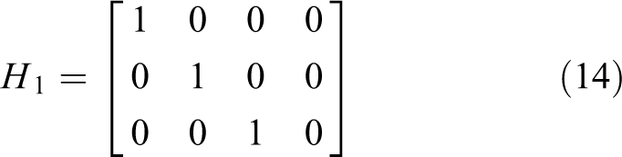
The matrix $T_{0}^{i}$ allows for calculating the position of the centre of mass coordinates for the link i in relation to the coordinate system of the base of the robotic manipulator per

c^{i} (q) = H_{1} T_{0}^{i} (q) Δ c^{i}

where H ₁ is defined as

H_{1} = [\begin{matrix} 1 & 0 & 0 & 0 \\ 0 & 1 & 0 & 0 \\ 0 & 0 & 1 & 0 \end{matrix}]

The tensor of inertia in relation to the base coordinate system is also determined as

D_{i} (q) = R_{0}^{i} (q) D_{i'} {[R_{0}^{i} (q)]}^{T}

Final step in the first part of the L-E algorithm is calculating the Jacobian matrix. The Jacobian matrix connects the infinitesimal movements of the manipulator joints to the infinitesimal movements of the tool and is defined using

J^{i} (q) = [\begin{array}{l} A^{k} (q) \\ B^{k} (q) \end{array}]

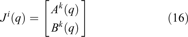
where matrices A and B are respectively defined with

A^{i} (q) = [\begin{matrix} \frac{\partial c^{i} (q)}{\partial q_{i}} & \dots & \frac{\partial c^{i} (q)}{\partial q_{i}} & 0 & \dots & 0 \end{matrix}]

and

B^{i} (q) = [\begin{matrix} θ_{1} z^{0} (q) & \dots & θ_{i} z^{i - 1} (q) & 0 & \dots & 0 \end{matrix}]

With these matrices calculated, the manipulator tensor of inertia can be determined as

D (q) = \sum_{i = 1}^{n} \{{[A^{i} (q)]}^{t} m_{i} [A^{i} (q)] + {[B^{i} (q)]}^{T} D_{i} (q) B^{k} (q)\}

When the manipulator’s tensor of inertia has been calculated, the value of the counter i is increased by one. If i is smaller or equal to n, where n is the number of joints of the robotic manipulator, the algorithm returns to the beginning of the process. If i is greater than n, the L-E algorithm proceeds with the second iterative part.

The beginning of the second iterative part is resetting the value of i to 1. Then, for the joint given by i, the speed connectivity matrix is calculated as

C_{k j}^{i} = \frac{\partial D_{i j} (q)}{\partial q_{k}} - \frac{1}{1} \frac{\partial D_{k j} (q)}{\partial q_{i}}, 1 \leq i, j, k \leq n

The gravity influence vector is calculated as

h_{i} (q) = - \sum_{k = 1}^{3} \sum_{j = 1}^{n} [g^{k} m_{j} A_{k} i^{j} (q)], 1 \leq i \leq n

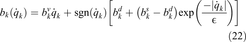
Furthermore, the friction is determined as

b_{k} ({\dot{q}}_{k}) = b_{k}^{v} {\dot{q}}_{k} + sgn ({\dot{q}}_{k}) [b_{k}^{d} + (b_{k}^{s} - b_{k}^{d}) exp (\frac{- |{\dot{q}}_{k}|}{ϵ})]

With this, all the necessary values are calculated and the L-E equation for the given link can be determined using

\begin{array}{l} τ_{i} = \sum_{j = 1}^{n} [D_{i j} (q) {\ddot{q}}_{j}] + \sum_{k = 1}^{3} \sum_{j = 1}^{n} [C_{k j}^{i} (q) {\dot{q}}_{k} {\dot{q}}_{j}] \\ + h_{i} (q) + b_{i} (q) \end{array}

The counter i is increased. If the value is smaller or equal to n, the algorithm returns to the first step of second iterative part and the calculation is repeated for the given link. If the value of i is greater than n, the L-E algorithm is finished.

N-E algorithm

N-E algorithm is a recursive method used to calculate the dynamic differential equations. It has two parts: the calculation ‘forward’ in which the linear and angular speeds and accelerations are calculated, and the calculation ‘backward’ in which the forces and momenta acting upon the link are calculated.⁴¹ In the calculation ‘forward’, the values are calculated for the links in the direction from the base of the robotic manipulator towards the tool, while in the calculation ‘backward’ the values are calculated from the direction from the tool to the base.^22,42,43 This is illustrated in Figure 3.

Figure 3.

The illustration of N-E algorithm.⁴⁴ N-E: Newton–Euler.

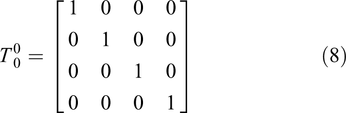
Before starting the calculation, the starting values need to be set to $T_{0}^{0} = I$ , $f^{n + 1} = - f^{tool}$ , $n^{n + 1} = - n^{tool}$ , $v^{0} = 0$ , $d v^{0} / d t = - g$ , $ω^{0} = 0$ , $d ω^{0} / d t = 0$ and counter $i = 1$ . When these values are set, the algorithm progresses into its first part – calculation ‘forward’.

The first part of the calculation ‘forward’ is the same as the start of the first iterative part of L-E algorithm in which the vector $z^{i - 1}$ is determined as

z^{i - 1} = R_{0}^{i - 1} * i^{3}

The next step is the calculation of the angular speed as

ω^{k} = ω^{i - 1} + ξ_{i} (\frac{d q_{i}}{d t}) z^{i - 1}

where $ξ_{i}$ is defined as

(\begin{array}{l} ξ_{i} = 1, & for revolutional joint \\ ξ_{i} = 0, & for linear joint \end{array}

Then the value of angular acceleration is calculated per

{\dot{ω}}^{i} = {\dot{ω}}^{i - 1} + ξ_{i} [(\frac{d^{2} q_{i}}{d t^{2}}) z^{i - 1} + ω^{i - 1} \times (\frac{d q_{i}}{d t} z^{i - 1})]

As in the L-E algorithm, the complex homogeneous transformation matrix is determined

T_{0}^{i} = T_{0}^{i - 1} T_{i - 1}^{k}

followed by the vector $Δ s$ as

Δ s^{i} = H_{1} (T_{0}^{i} - T_{0}^{i + 1}) i^{4}

Final part of calculation forward is calculating the linear acceleration using

\begin{array}{l} \frac{d v^{i}}{d t} = \frac{d v^{i - 1}}{d t} + \frac{d ω^{i}}{d t} \times Δ s^{i} + ω^{i} \times (ω^{i} \times Δ s^{i}) \\ + (1 - ξ_{i}) [\frac{d^{2} q_{i}}{d t^{2}} z^{i - 1} + 2 ω^{i} \times ({\dot{q}}_{i} z^{i - 1})] \end{array}

After the linear acceleration is calculated, the counter i is increased by one. If the value of i is lesser than n, the calculation repeats for the next link. If the value is greater than n, the algorithm proceeds to the calculation ‘backward’. Calculation ‘backward’ is started by calculating the vector r^k

Δ r^{k} = H_{1} T_{0}^{k} (Δ c^{k} - i^{4})

and the tensor of inertia of the robotic manipulator link given by i in relation to the base of robotic manipulator

D_{k} = R_{0}^{k} D_{k}^{′} {(R_{0}^{k})}^{T}

Then the forces and the momentum acting upon the link given by i are calculated as

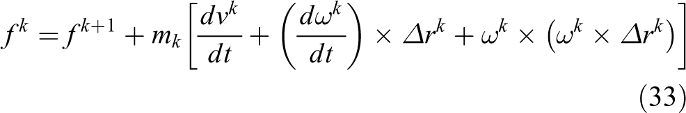
f^{k} = f^{k + 1} + m_{k} [\frac{d v^{k}}{d t} + (\frac{d ω^{k}}{d t}) \times Δ r^{k} + ω^{k} \times (ω^{k} \times Δ r^{k})]

and

\begin{array}{l} n^{k} = n^{k + 1} + (Δ s^{k} + Δ r^{k}) \times f^{k} - Δ r^{k} \times f^{k + 1} + D_{k} (\frac{d ω^{k}}{d t}) + ω^{k} \times (D_{k} ω^{k}) \end{array}

The final calculation is determining the value of the joint actuator momentum using the equation

τ_{k} = ξ_{k} {(n^{k})}^{T} z^{k - 1} + (1 - ξ_{k}) {(f^{k})}^{T} z^{k - 1} + b_{k} ({\dot{q}}_{k})

The value of i is then lowered by one. If the value of i is larger than zero, the calculation ‘backward’ is repeated for the next joint. If the value of i is zero, the base of the robotic manipulator has been reached and the N-E algorithm is finished.

Used algorithms

In this article, five different algorithms were utilized and these are:

GA with average recombination,

GA with random recombination,

SA with linear cooling strategy,

SA with geometric cooling strategy and

DE.

Used algorithms will be discussed in this chapter.

All of the above are evolutional computing algorithms, which are based on performing the iterative method on a certain population of agents to achieve an optimal result from the solution space. Solution space is defined as the n-dimensional mathematical space containing all the possible solutions to a given problem,^45,46 with each solution having a value calculated with a fitness function defining how well does the given solution satisfy the conditions given for solving the problem.^47,48 Each agent is a point in the solution space – an instance of a solution containing genotype data. Genotype is the simplified representation of the solution to the given problem which is the phenotype of the problem.⁴⁹ In this article, phenotype is the movement of the robotic manipulator through the space, while the genotype is the parameters of equations that describe the movement of the robotic manipulator. A group of agents upon which the optimization is performed is called the population ^50,51 and each iteration of the evolutionary algorithm is called a generation. ⁵² All algorithms end when an end condition ^53,54 is fulfilled. End condition is usually fulfilled after a certain amount of generations have passed or when there was not a change in the best achieved value of fitness function for a certain amount of generations.⁵⁵ All algorithms are run with population of 20 agents for the period of 50 generations.

Genetic algorithm

GA is an optimization algorithm that imitates the process of biological evolution using the mechanisms of crossover and mutation.^55,56

Crossover is a mechanism in which the new agent (child) is created by randomly choosing two existing agents from the population (parents) and generating the values of parameters of the child agent from the values of parameters of parent agents. The idea of crossover is that by generating new agents, and consistently keeping the better fitting agents in the population, through the recombination of agents, the optimal solution will be found.⁵⁶ The wish is for the crossover to result in the better fitting gene which will replace a worse fitting agent currently in the population. If the new agent is not of a higher quality, then the current gene is kept.^57,58

There are multiple ways to cross the agent’s parameters to generate a new agent. In this article, two mechanisms are used: random recombination and average recombination.^59,60

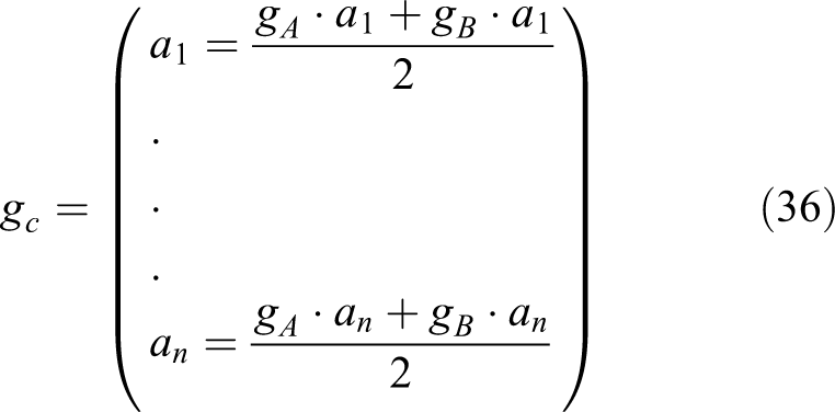
When using the average recombination, the values of child agent’s (g_c ) parameters (a_i ) are calculated as the average value of the parameter of the parent agents (g_A and g_B ). This is given as

g_{c} = (\begin{array}{l} a_{1} = \frac{g_{A} \cdot a_{1} + g_{B} \cdot a_{1}}{2} \\ . \\ . \\ . \\ a_{n} = \frac{g_{A} \cdot a_{n} + g_{B} \cdot a_{n}}{2} \end{array})

In the case of random recombination, the parameter values of the child agent are randomly chosen between the appropriate parameter values of the two parent agents, as

g_{c} = (\begin{array}{l} a_{1} \cap \{g_{A} \cdot a_{1}, g_{B} \cdot a_{1}\} \\ . \\ . \\ . \\ a_{n} \cap \{g_{A} \cdot a_{n}, g_{B} \cdot a_{n}\} \end{array})

Mutation is the process in which an agent’s parameters are randomly chosen from the solution space and the agent created in that way replaces an agent in the population, with no attention paid to the fitness function values – so a worse mutated agent can replace the better one.⁴⁵ The mutation mechanism is necessary to avoid the stagnation that can happen when only the crossover mechanism is implemented. It allows the GA to move away from the situation where all the agents are in the local optimum of solution space and give it ability to find the global optimum.⁶¹ Mutation is used in a low amount of cases (1% of the iterations), as opposed to the crossover which is used comparatively often (80% of the iterations).^62,63

The described procedure of GA is shown in Figure 4.

Figure 4.

Flow chart of GA. GA: genetic algorithm.

Simulated annealing

SA is an optimization algorithm inspired by the process of metal annealing. The SA algorithm has a system temperature which lowers, according to the cooling strategy, through the algorithm iterations.^64,65 The algorithm selects a solution from the neighbouring solution space to the current solution and, if that solution is better, replaces the current solution with it. The system temperature determines the likelihood of the algorithm accepting the worse solution. The likelihood of the worse solution being chosen is proportional to the system temperature. This is usually implemented by generating a random value in the possible temperature range and accepting a worse solution if that value is lower than the current temperature. This mechanism serves a similar purpose as the mutation mechanism does in the GA. This gives the SA algorithm the capability to select a different solution if the current solution is located in the local minimum of the solution space.^66,67

The likelihood of choosing a worse solution at some point of the algorithm execution can be configured by choosing a cooling strategy.⁶⁸ Two strategies are used in this article - linear as shown

t_{k} = t_{0} - α k

and geometric strategy as

t_{k} = t_{0} * β^{k}

where k is the current algorithm iteration, t_k is the current system temperature, t ₀ is the starting system temperature and α and $β$ are cooling factors which determine the speed at which the system cools.⁶⁹ The process which SA algorithm uses to find the optimal solution is shown in Figure 5. In this article, the starting temperature of the SA algorithm is set to 100, with the coefficient α for linear cooling strategy being set to 1, and coefficient $β$ for geometric cooling strategy being set to 0.5.

Figure 5.

Flow chart of SA. SA: simulated annealing.

Differential evolution

DE is an AI optimization algorithm, which uses differential equations as the inspiration. This algorithm is particularly fitting for the solution spaces that are not smooth and have interruptions.^70,71 DE algorithm creates a new agent by combining three agents using

g_{y} = (\begin{array}{l} a_{1} = g_{a} \cdot a_{1} + F * (g_{b} \cdot a_{1} - g_{c} \cdot a_{1}) \\ . \\ . \\ . \\ a_{n} = g_{a} \cdot a_{n} + F * (g_{b} \cdot a_{n} - g_{c} \cdot a_{n}) \end{array})

where F is a constant that determines how distant the new solution will be in the solution space from a randomly selected agent g_a , and has a value in range $F \in 〈 0, 2]$ .^72,73

Three agents are randomly picked from the population and the values of new agent are calculated. If the value of the new agent is better than the agent in the current iteration, it replaces the current agent.⁷⁰ Unlike SA algorithm, DE does not have a mechanism which allows it to select a worse solution, nor does it have a mechanism similar to mutation such as can be seen in GA. DE avoids stagnation by having a large search area (configured by parameter F).⁷⁴ A larger value of the parameter F will give a larger search area, but will increase the time it takes for the algorithm to converge to a solution, while the smaller value will cause a faster convergence to a solution, but it will be more likely the found solution will be a local instead of a global optimum. In this research, parameter F is set to 1.2, which is the starting value used in most research.⁷¹ The process of DE algorithm is shown in Figure 6.

Figure 6.

Flow chart of DE algorithm. DE: differential evolution.

Agent construction

In the cases observed in this article, the phenotype of the robotic manipulator movement is represented with a parameter of the equation describing that movement as^75
–77

θ (q) = a t^{4} + b t^{3} + c t^{2} + d t + e

Parameters b, c, d, and e can be removed from the equation if the following conditions are observed^22,77: the starting time is zero ( $t_{s} = 0 s$ ) and the movement lasts 2 s ( $t_{f} = 2 s$ ) the robotic manipulator joints move from 0 radian to 1 radian ( $θ (0) = 0$ rad, $θ (2) = 1$ rad), it starts movement as stationary – the starting speeds and accelerations are zero ( $v (t_{s}) = 0$ m/s, $\frac{d v}{d t} (t_{s}) = 0$ m/s², $ω (t_{s}) = 0$ rad/s, $\frac{d ω}{d t} (t_{s}) = 0$ rad/s²) and it ends the movement stationary – the ending speeds and accelerations are equal to zero ( $v (t_{f}) = 0$ m/s, $\frac{d v}{d t} (t_{f}) = 0$ m/s², $ω (t_{f}) = 0$ rad/s, $\frac{d ω}{d t} (t_{f}) = 0$ rad/s²).

The parameter e is eliminated using the condition that the starting joint angle equals 0

\begin{array}{l} t & = 0 \\ q (0) & = 0 \\ q (0) & = a * 0^{4} + b * 0^{3} + c * 0^{2} + d * 0 + e \\ q (0) & = e \Rightarrow e = 0 \end{array}

Parameter d can be eliminated by the derivation of equation (41) to get the equation describing the angular joint velocity and using the starting condition of initial angular joint velocity being 0

\begin{array}{l} ω (t) & = \frac{d q}{d t} \\ ω (t) & = 4 a t^{3} + 3 b t^{2} + 2 c t + d \\ t & = 0 \\ ω (0) & = 0 \\ ω (0) & = 4 a * 0^{3} + 3 b * 0^{2} + 2 c * 0 + d \\ ω (0) & = d \Rightarrow d = 0 \end{array}

Second derivation of equation (41) is the expression for the joint’s angular acceleration is derived. If the condition that the initial joint’s angular acceleration is zero is used, the parameter c is eliminated per

\begin{array}{l} \frac{d ω}{d t} (t) & = \frac{d^{2} q}{d t^{2}} \\ \frac{d ω}{d t} (t) & = 12 a t^{2} + 6 b t + 2 c \\ t & = 0 \\ \frac{d ω}{d t} (0) & = 0 \\ \frac{d ω}{d t} (0) & = 12 a * 0^{2} + 6 b * 0 + 2 c \\ \frac{d ω}{d t} (0) & = 2 c \Rightarrow c = 0 \end{array}

Parameter b can be defined using

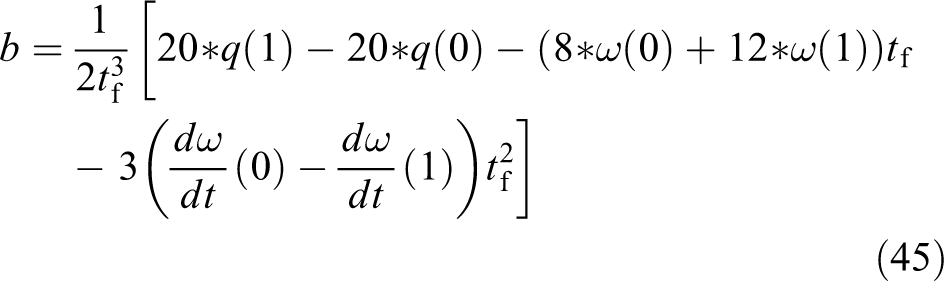
b = \frac{1}{2 t_{f}^{3}} [20 * q (1) - 20 * q (0) - (8 * ω (0) + 12 * ω (1)) t_{f} - 3 (\frac{d ω}{d t} (0) - \frac{d ω}{d t} (1)) t_{f}^{2}]

By inserting the starting and ending conditions, parameter b can be eliminated per

\begin{array}{l} b = \frac{1}{2 * 1^{3}} [20 * 1 - 20 * 0 - (8 * 0 + 12 * 0) * 1 - 3 (0 - 0) * 1^{2}] \\ b = \frac{1}{2} * 20 \Rightarrow b = 10 \end{array}

making it equal to a constant.

With these parameters eliminated, the only remaining parameter is parameter a which will describe the movement of each joint of the robotic manipulator.

In the case of the single robotic manipulator, the joint movements are described by six parameters a_i , where i is the joint number. Since this is the parameter used for optimization, it can be referred to as optimization parameter. In the case of two robotic manipulators, the joint movements need to be calculated using the inverse kinematic equations. The values of vector w are calculated according to equations (4) to (6). Vector w contains the equations containing values of all six joints. The joint variables (q ₁, q ₂, q ₃, q ₄, q ₅ and q ₆) can be extracted from these equations which gives a set of six inverse kinematic equations that define the joint values as function of the end-effector position in space (vector w).^78
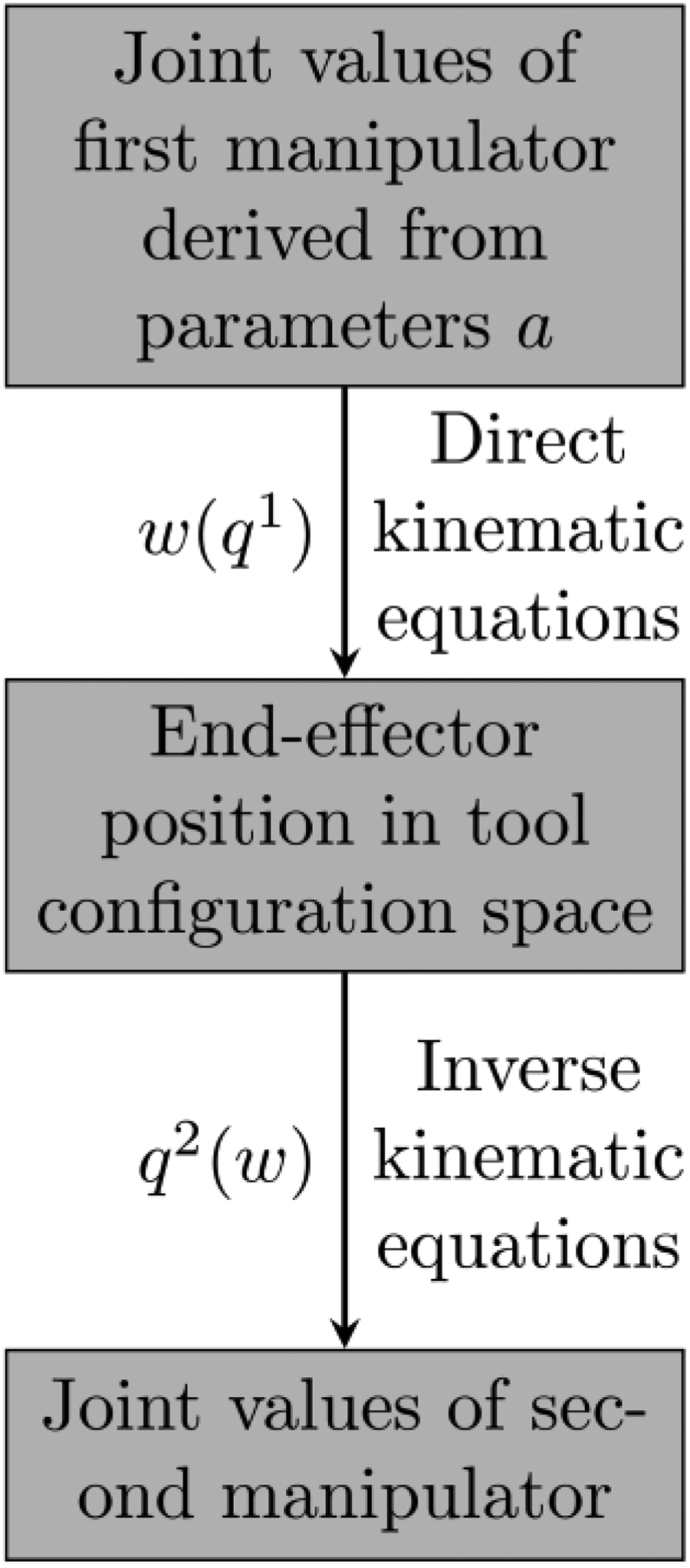
–80 By entering the values of vector w into these inverse kinematic equations, it is possible to get the values of joint variables needed to achieve the position described by vector w. Hence, if the joint variable values of the first robotic manipulator ( $q_{1}^{1}$ , $q_{2}^{1}$ , $q_{3}^{1}$ , $q_{4}^{1}$ , $q_{5}^{1}$ and $q_{6}^{1}$ ) are determined from the optimization parameters a_i , the direct kinematic equations (5) and (6) can be used to determine the position of end-effector in the space, defined by vector w.^21,38 Using the inverse kinematic equations to determine the joint variables of second robotic manipulator ( $q_{1}^{2} (w)$ , $q_{2}^{2} (w)$ , $q_{3}^{2} (w)$ , $q_{4}^{2} (w)$ , $q_{5}^{2} (w)$ and $q_{6}^{2} (w)$ ) will result in the end-effector position of the second robotic manipulator following the positioning of the first robotic manipulator, enabling cooperative behaviour.^39,76,78 This process is shown in Figure 7.

Figure 7.

Process of allowing calculating the second robotic manipulator joint values to achieve cooperative behaviour.

That means that in both observed cases generating only a single set of parameters a_i (one for each joint) is necessary, as those will be used for determining the movement of the first robot and the second robotic manipulator’s movement will be determined by the movement of the first, which gives the genotype shape defined by

g = \{a_{1}, a_{2}, a_{3}, a_{4}, a_{5}, a_{6}\}

where a_i is part of the interval

a_{i} \in [- 10, 10]

Fitness function

To be able to determine how well does each agent solve a problem, it is necessary to define a fitness function which will provide a value describing it.

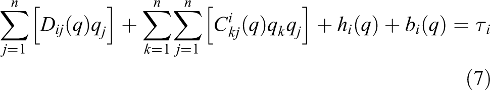
In this instance, the fitness function is defined as the sum of the total torsion on each point of the trajectory, where the total joint torque is defined as the sum of joint torques on each joint of the robotic manipulator(s).⁷ This is defined by the equation

f (g) = \sum_{m = 1}^{M} \sqrt{\sum_{i = 1}^{n} τ_{i}^{2}},

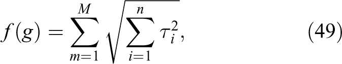
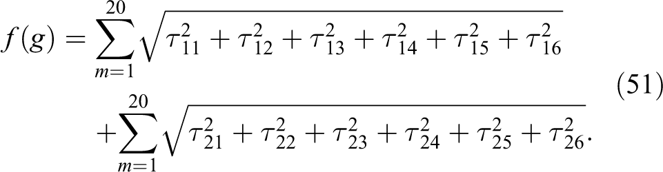
where M is the number of points in the trajectory, n is the total number of joints of the robotic manipulator and $τ_{i}$ is torque of the ith joint. Squaring each torque and taking the square root of their sum in each step of the trajectory provides the absolute value of all joint torques acting on the robotic manipulator.

Since the observed cases in this article have 20 points in their trajectory and n is either 6 (in the case of a single robotic manipulator) or 12 (in the case of the two cooperating robotic manipulators), the fitness function for each of the two cases can be defined for the case with the single robotic manipulator as

f (g) = \sum_{m = 1}^{20} \sqrt{τ_{1}^{2} + τ_{2}^{2} + τ_{3}^{2} + τ_{4}^{2} + τ_{5}^{2} + τ_{6}^{2}},

and for the case with two cooperating robotic manipulators as

\begin{matrix} f (g) = & \sum_{m = 1}^{20} \sqrt{τ_{11}^{2} + τ_{12}^{2} + τ_{13}^{2} + τ_{14}^{2} + τ_{15}^{2} + τ_{16}^{2}} \\ + \sum_{m = 1}^{20} \sqrt{τ_{21}^{2} + τ_{22}^{2} + τ_{23}^{2} + τ_{24}^{2} + τ_{25}^{2} + τ_{26}^{2}} . \end{matrix}

Results

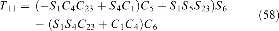
The result of the D-H method can be written in the following form

T_{0}^{6} = [\begin{matrix} T_{00} & T_{01} & T_{02} & T_{04} \\ T_{10} & T_{11} & T_{12} & T_{14} \\ T_{20} & T_{21} & T_{22} & T_{24} \\ T_{30} & T_{31} & T_{32} & T_{34} \end{matrix}]

where

\begin{matrix} T_{00} = & ((S_{1} S_{4} + C_{1} C_{4} C_{23}) C_{5} - S_{5} S_{23} C_{1}) C_{6} \\ + (S_{1} C_{4} - S_{4} C_{1} C_{23}) S_{6} \end{matrix}

\begin{array}{l} T_{10} = & ((S_{1} C_{4} C_{23} - S_{4} C_{1}) C_{5} - S_{1} S_{5} S_{23}) C_{6} \\ - (S_{1} S_{4} C_{23} + C_{1} C_{4}) S_{6} \end{array}

T_{20} = - (S_{5} C_{23} + S_{23} C_{4} C_{5}) C_{6} + S_{4} S_{6} S_{23}

T_{30} = 0

\begin{array}{l} T_{01} = & (- (S_{1} S_{4} + C_{1} C_{4} C_{23}) C_{5} + S_{5} S_{23} C_{1}) S_{6} \\ + (S_{1} C_{4} - S_{4} C_{1} C_{23}) C_{6} \end{array}

\begin{array}{l} T_{11} = & (- S_{1} C_{4} C_{23} + S_{4} C_{1}) C_{5} + S_{1} S_{5} S_{23}) S_{6} \\ - (S_{1} S_{4} C_{23} + C_{1} C_{4}) C_{6} \end{array}

T_{21} = (S_{5} C_{23} + S_{23} C_{4} C_{5}) S_{6} + S_{4} S_{23} C_{6}

T_{31} = 0

T_{02} = - (S_{1} S_{4} + C_{1} C_{4} C_{23}) S_{5} - S_{23} C_{1} C_{5}

T_{12} = (- S_{1} C_{4} C_{23} + S_{4} C_{1}) S_{5} - S_{1} S_{23} C_{5}

T_{22} = S_{5} S_{23} C_{4} - C_{5} C_{23}

T_{32} = 0

\begin{array}{l} T_{03} = & - l_{4} S_{1} S_{4} S_{5} - l_{4} S_{5} C_{1} C_{4} C_{23} - l_{4} S_{23} C_{1} C_{5} \\ - l_{1} S_{23} C_{1} + l_{3} C_{1} C_{2} + l_{5} C_{1} C_{23} \end{array}

\begin{array}{l} T_{13} = & - l_{4} S_{1} S_{5} C_{4} C_{23} - l_{4} S_{1} S_{23} C_{5} - l_{1} S_{1} S_{23} \\ + l_{3} S_{1} C_{2} + l_{5} S_{1} C_{23} + l_{4} S_{4} S_{5} C_{1} \end{array}

\begin{array}{l} T_{23} = & - l_{3} S_{2} + l_{4} S_{5} S_{23} C_{4} - l_{5} S_{23} - l_{4} C_{5} C_{23} \\ - l_{1} C_{23} + l_{2} \end{array}

T_{33} = 1

In the results, the algorithms used are given shortened names: GA-A represents the GA with average recombination, GA-R represents the GA with random recombination, SA-L represents the SA algorithm with linear cooling strategy and SA-G represents SA with geometric cooling strategy.

The comparison of results between algorithms is given in Table 1. The best results and shortest execution times are shown in bold in the table for emphasis. In Table 1, $\bar{Δ}$ represents the average over multiple runs of the difference between the best fitness value from the initial randomly picked population and the best fitness value from the final optimized population, $Δ = f (g_{p_{1}}) - f (g_{p_{50}})$ .

Table 1.

Result comparison between used algorithms and their execution times in both observed cases.

	Single manipulator		Dual manipulators
	$\bar{Δ}$ Nm	$\bar{t}$ m:s	$\bar{Δ}$ Nm	$\bar{t}$ h:m:s
GA-A	104.78	02:28	86.09	05:55:43
GA-R	177.96	02:17	54.84	06:50:38
SA-L	70.25	20.16	36.79	10:56:49
SA-G	100.82	08:20	14.94	17:03:10
DE	165.49	02:18	63.44	05:58:40

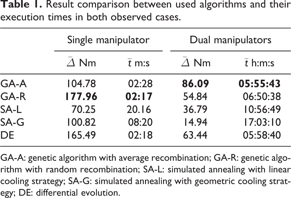
GA-A: genetic algorithm with average recombination; GA-R: genetic algorithm with random recombination; SA-L: simulated annealing with linear cooling strategy; SA-G: simulated annealing with geometric cooling strategy; DE: differential evolution.

In Figure 8, a drop in the fitness function value is shown, which was calculated using equation (49), as is expected – considering this is an optimization problem which has the goal of lowering the value of fitness function which represents the total joint torques of robotic manipulators. The fitness shown is the fitness function value of the best agent in the population of 20 agents in the given generation. The initial drop to a better solution happens in the first few generations, with a further drop down before the 30th generation. The last drop of the fitness function value happens around the 35th generation and then it stays at the lowest optimized value. Figure 8 shows a significant drop in the fitness function value, most probably due to a rather suboptimal initial randomly selected solution.

Figure 8.

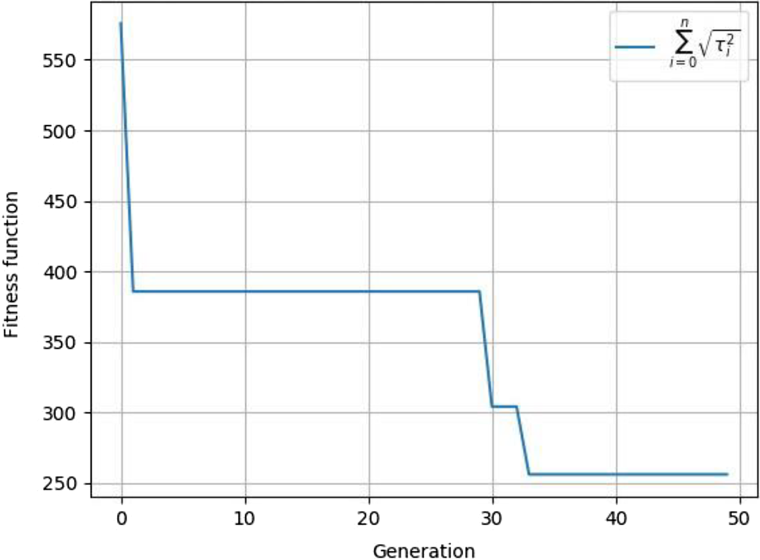
Example of the change of the fitness function through the generations for a case with a single robotic manipulator.

In Figure 9, the joint trajectory after the optimization process is shown. It can be seen that the joints start at the position of 0 radian and end in the position of 1 radian. The calculated joint trajectories are smooth, without any sudden jumps and changes that would cause large differences in joint torques or generate sudden movements of the robotic manipulator.

Figure 9.

Joint trajectory for the case of a single robotic manipulator.

Figures 10 and 11 show the resultant trajectories of joints of robotic manipulators in the case with two cooperating robotic manipulators. The joint trajectories for the case of two cooperating robotic manipulators have been shown on two separate figures for easier viewing. Trajectories of both robotic manipulators show smooth curves.

Figure 10.

Joint trajectory for the case of a cooperative robotic motion for first robotic manipulator.

Figure 11.

Joint trajectory for the case of a cooperative robotic motion for second robotic manipulator.

Figure 12 shows the change of joint torque on each joint of the robotic manipulator. It can be seen that in the optimal case found in this particular optimization run, the joint torque shows a drop into negative values followed by a smooth raise. The smooth changes in the joint torques like these have shown to be common when using SA algorithms. The joint torque of the second joint exhibits the highest rise, caused by the robotic manipulator configuration where the second joint is placed under most stress.

Figure 12.

Change of joint torques over the trajectory for the case of a single robotic manipulator.

Figures 13 and 14 show the change of joint torques on the first and second robotic manipulator. As with the joint trajectories for dual manipulators, the joint torques have been split into two figures for easier viewing. Some sudden changes can be seen in the direction of the joint torques (observe 14 at 0.5 s). This is prominent with the use of GA and DE for the optimization process. The sudden changes like these are also especially prominent on the second robotic manipulator for which the joint angles are determined using inverse kinematics as opposed to the first manipulator for which the joint angles are determined using equation (41). On both robotic manipulators, joint torque of the second robotic manipulator joint shows the highest torque, which is caused by the robotic manipulator configuration.

Figure 13.

Change of joint torques over the trajectory in the case of a cooperative robotic motion for the first dual robotic manipulator.

Figure 14.

Change of joint torques over the trajectory in the case of a cooperative robotic motion for the second dual robotic manipulator.

Discussion

The results show a successful decrease in the total joint torque in the robotic manipulator in comparison with the initial randomly selected parameters. The best results and the fastest execution time are shown by the GA using average recombination for the dual cooperating manipulator and random recombination for the case with the single manipulator. The DE shows good results in both cases, having better results than the average recombination GA in the single manipulator case and better results than the random recombination algorithm in the dual manipulator case. DE shows fast execution times in both cases, comparable with the GA. SA shows mixed results, with the linear cooling strategy showing the weakest results in both cases. The SA with geometric cooling strategy shows results comparable with the average recombination GA (although significantly weaker compared to the random recombination GA) in the single manipulator case, but it shows the weakest results in the dual manipulator case. SA shows the longest execution time necessary to complete optimization, with the linear cooling strategy being the longest running algorithm of all compared in this article. The results consistently show that the largest joint torque is the torque of the second joint of the robotic manipulator ( $τ_{2}$ ). These large torque values are caused due to the configuration of the robotic manipulator where the second joint has most stress placed on it during the movement of the robotic manipulator. This can be observed when optimizing with all used algorithms, and is especially pronounced when optimizing with DE. Large values of joint torques near the end of the trajectory that sometimes happen are caused by the fact that the end conditions guarantee the robotic manipulator ending its movement in the defined position, making it harder to optimize the trajectory near the end of the movement. It is important to note that, despite providing the weakest improvements in regard to the amount of total joint torque lowered, the SA (in both configurations) is the only algorithm that provides results with the smooth torque and joint curves in almost all instances. The curves provided by the GA have a tendency to show sudden changes in joint torque, which can negatively impact the durability of the robotic manipulator, while the ones provided by the DE have a tendency to have one of the joints of the robotic manipulator have a high torque, with very low joint torques on the other joints. While this does result in a low total joint torque, it might not be appropriate depending on the robotic manipulator used. This points towards the SA being the best algorithm for producing a smooth joint torque curves after the optimization.

Conclusion

The results show a successful optimization in both observed cases using evolutionary algorithms. The best results among the used algorithms are provided using GA with random recombination for single robotic manipulator and with average recombination for dual cooperating manipulators. DE has also shown good results in comparison with other algorithms. For the objectives optimized in this article, SA shows the worst results. But, the generated results are not optimal in regard to the smoothness of the curves, where SA shows the best results in comparison with other algorithms used, and stress placed on second joint of robotic manipulator(s). This article shows successful application of evolutionary algorithms on the problem of path optimization of the realistic six-DOF robotic manipulator, where earlier research had only shown application on simpler manipulators. In practice, this means that by applying evolutionary algorithms to perform optimization on the planned paths, the amount of energy used for the robotic manipulators to perform work could be lowered, as well as the longevity of the robotic manipulators raised due to less damages caused by the torsion developed in the joints during the movement. The work done in the article does come with certain limitations. First is that the dynamic model used is not general. While this means the optimization results are high quality for the used robotic manipulator, it also means that to apply the algorithms described on a different robotic manipulator entire dynamics need to be recalculated to be used for optimization. Additionally, this article describes methods as used on the point-to-point planning, and do not apply to widely used continuous path planning – which would require the way joints values are calculated to be adjusted. Future work could concentrate on multi-objective optimization that would attempt to lower the joint torques as one objective, and provide a smooth curve as the other and more equal joint torque distribution. Additionally, future work could concentrate on wider parameter variations, friction implementation and continuous path planning. Instead of using the recommended algorithm parameter values, such as they were in this article, performance of algorithms could be tested with different variations of their parameters in an attempt to increase the performance further. Friction, as mentioned, was not included in the model used in this article, because of complexity of determining the appropriate friction model. Friction in the manipulator could be modelled using different approaches, and the influence of them on the optimization process measured. Finally, while point-to-point path planning has wide applications, modifying the algorithm to perform optimization over continuous paths could provide wider application for this research.

Footnotes

Declaration of conflicting interests

The author(s) declared no potential conflicts of interest with respect to the research, authorship, and/or publication of this article.

Funding

The author(s) disclosed receipt of the following financial support for the research, authorship, and/or publication of this article: This research has been (partly) supported by the CEEPUS network CIII-HR-0108, European Regional Development Fund under the grant KK.01.1.1.01.0009 (DATACROSS), University of Rijeka scientific grant uniri-tehnic-18-275-1447 and the project VEGA 1/0504/17.

ORCID iD

Zlatan Car

References

Pfeiffer

Johanni

. A concept for manipulator trajectory planning. IEEE J Robot Autom 1987; 3(2): 115–123.

Wang

. Design and fabrication of a soft robotic manipulator driven by fiber-reinforced actuators. In: 2018 IEEE international conference on mechatronics, robotics and automation (ICMRA), Hefei, China, 18–21 May 2018, pp. 157–161. IEEE.

Sharma

Singh

. Optimization of energy in robotic arm using genetic algorithm. Int J Comp Sci Technol 2011; 2(2): 315–317.

Kazem

Mahdi

Oudah

. Motion planning for a robot arm by using genetic algorithm. Jjmie 2008; 2(3): 131–136.

Albert

Koh

Chen

, et al. Optimizing joint angles of robotic manipulator using genetic algorithm. In: International conference on computer engineering and applications IPCSIT (ed Othman

), vol. 2. 2011, pp. 134–140. Singapore: IACSIT Press.

Nassehi

Essink

Barclay

. Evolutionary algorithms for generation and optimization of tool paths. CIRP Annals 2015; 64(1): 455–458.

Garg

Kumar

. Optimization techniques applied to multiple manipulators for path planning and torque minimization. Eng Appl Artif Intel 2002; 15(3–4): 241–252.

Wei

Hiraga

Ohkura

, et al. Autonomous task allocation by artificial evolution for robotic swarms in complex tasks. Artif Life Robot 2019; 24(1): 127–134.

Abu-Dakka

Assad

Alkhdour

, et al. Statistical evaluation of an evolutionary algorithm for minimum time trajectory planning problem for industrial robots. Int J Adv Manuf Technol 2017; 89(1–4): 389–406.

10.

Larsen

Schuster

Kim

, et al. Path planning of cooperating industrial robots using evolutionary algorithms. Procedia Manuf 2018; 17: 286–293.

11.

Wei

Nie

Hiraga

, et al. Developing end-to-end control policies for robotic swarms using deep Q-learning. J Adv Comput Intel Intel Inform 2019; 23(5): 920–927.

12.

El Haiek

Aboulissane

El Bakkali

, et al. Optimal trajectory planning for spherical robot using evolutionary algorithms. Procedia Manuf 2019; 32: 960–968.

13.

Mirjalili

Genetic algorithm. In: Kacprzyk

(ed.) Evolutionary algorithms and neural networks. Berlin: Springer, 2019, pp. 43–55.

14.

Zhao

Zhu

Luo

. Multitask-based trajectory planning for redundant space robotics using improved genetic algorithm. Appl Sci 2019; 9(11): 2226.

15.

Fang

Ming

, et al. Multi-objective evolutionary simulated annealing optimisation for mixed-model multi-robotic disassembly line balancing with interval processing time. Int J Prod Res 2019; 58(3): 846–862.

16.

Sakamoto

Ozera

Barolli

, et al. Implementation of an intelligent hybrid simulation systems for WMNs based on particle swarm optimization and simulated annealing: performance evaluation for different replacement methods. Soft Comput 2019; 23(9): 3029–3035.

17.

Back

Fogel

Michalewicz

. Evolutionary computation 1: basic algorithms and operators. Florida: CRC Press, 2018.

18.

Prabhu

SGR

Seals

Kyberd

, et al. A survey on evolutionary-aided design in robotics. Robotica 2018; 36(12): 1804–1821.

19.

Atta

Mahapatra

PRS

Mukhopadhyay

. Deterministic and randomized heuristic algorithms for uncapacitated facility location problem. In: Satapathy

Tavares

Bhateja

Mohanty

(eds) Information and decision sciences. Berlin: Springer, 2018, pp. 205–216.

20.

Car

Mikac

. Evolutionary approach for solving cell-formation problem in cell manufacturing. Adv Eng Inform 2006; 20(3): 227–232.

21.

Lopes

Pires

Barbosa

. Design of a parallel robotic manipulator using evolutionary computing. Int J Adv Robot Syst 2012; 9(1): 27.

22.

Yoshikawa

. Foundations of robotics: analysis and control. Cambridge, MA: MIT Press, 1990.

23.

de Farias

da Cruz Figueredo

Ishihara

. Performance study on dqRNEA – a novel dual quaternion based recursive Newton-Euler inverse dynamics algorithms. In 2019 third IEEE international conference on robotic computing (IRC), Naples, Italy, 25–27 February 2019, pp. 94–101. IEEE.

24.

Al-Shuka

Corves

Zhu

. Dynamics of biped robots during a complete gait cycle: Euler-Lagrange vs. Newton-Euler formulations. School of Control Science and Engineering. Shandong University, 2019, pp. 1–39. https://hal.archives-ouvertes.fr/hal-01926090/document (accessed 18 February 2020).

25.

Tsai

LW.

Robot analysis: the mechanics of serial and parallel manipulators. New Jersey: John Wiley and Sons, 1999.

26.

Spong

Vidyasagar

. Robot dynamics and control. New Jersey: John Wiley and Sons, 2008.

27.

Becerra

Arbulu

Soto

, et al. A comparison among the Denavit-Hartenberg, the screw theory, and the iterative methods to solve inverse kinematics for assistant robot arm. In: International conference on swarm intelligence (eds Tan

Shi

Niu

), Chiang Mai, Thailand, 26–30 July 2019, pp. 447–457. New York: Springer.

28.

Corke

. A simple and systematic approach to assigning Denavit–Hartenberg parameters. IEEE Trans Robot 2007; 23(3): 590–594.

29.

Kim

Mishra

Limosani

, et al. Control strategies for cleaning robots in domestic applications: a comprehensive review. Int J Adv Robot Syst 2019; 16(4): 1–21. DOI: 10.1177/1729881419857432.

30.

Gao

Sun

, et al. Structural parameter identification for 6 DOF industrial robots. Mech Syst Signal Process 2018; 113: 145–155.

31.

Cristoiu

Nicolescu

. New approach for forward kinematic modeling of industrial robots. Res and Sci Today 2017; 13: 136.

32.

Valayil

Selladurai

Ramaswamy

. Kinematic modeling of a serial robot using Denavit-Hartenberg method in Matlab. (TAGA) Journal of grahic technology 2018; 14: 2347–2445. http://www.tagajournal.com/gallery/v14.230.pdf (accessed 18 February 2020).

33.

Klug

Schmalstieg

Gloor

, et al. A complete workflow for automatic forward kinematics model extraction of robotic total stations using the Denavit-Hartenberg convention. J Intel Robot Syst 2019; 95(2): 311–329.

34.

Parker

Khoogar

Goldberg

. Inverse kinematics of redundant robots using genetic algorithms. In: Proceedings, 1989 international conference on robotics and automation, Scottsdale, AZ, USA, 14–19 May 1989, pp. 271–276. IEEE.

35.

Diebel

Representing attitude: Euler angles, unit quaternions, and rotation vectors. Matrix 2006; 58(15–16): 1–35.

36.

Khomchenko

. Robot manipulator end-effector orientation setting methods. Journal of Physics: Conference Series 2019; 1210: 012062.

37.

Petrescu

. Direct and inverse kinematics to the anthropomorphic robots. Engevista 2016; 18: 109–124.

38.

Hussain

Awad

Junaid

, et al. Dynamic modeling and numerical simulations of a passive robotic walker using Euler-Lagrange method. In: 2018 11th international symposium on mechatronics and its applications (ISMA), Sharjah, United Arab Emirates, 4–6 March 2018, pp. 1–6. IEEE.

39.

Lewis

Dawson

Abdallah

. Robot manipulator control: theory and practice. Florida: CRC Press, 2003.

40.

Kurfess

TR.

Lagrangian dynamics. In: Kurfess

(ed.) Robotics and automation handbook. Florida: CRC Press, 2018, pp. 73–88.

41.

Hwang

Cheng

Truong

. Dynamic analysis and control of industrial robotic manipulators. In: Applied mechanics and materials. Vol. 883. Switzerland: Trans Tech Publications Ltd, 2018, pp. 30–36.

42.

Nagurka

ML.

Newton-Euler dynamics of robots. In: Kurfess

(ed.) Robotics and Automation Handbook. Florida: CRC Press, 2018, pp. 63–72.

43.

Valverde

Tsiotras

. Modeling of spacecraft-mounted robot dynamics and control using dual quaternions. In: 2018 annual American control conference (ACC) (ed Spall

), Milwaukee, WI, USA, 27–29 June 2018, pp. 670–675. IEEE.

44.

ABB, Affolternstrasse 44 8050 Zurich Switzerland. Product Specification IRB-120, t ed, 2019.

45.

Mohammed

Ghani

MKA

Hamed

, et al. Solving vehicle routing problem by using improved genetic algorithm for optimal solution. J Comput Sci 2017; 21: 255–262.

46.

Xie

Yuille

. Genetic CNN. In: Proceedings of the IEEE international conference on computer vision, Venice, Italy, 22–29 October 2017, pp. 1379–1388. Piscataway, NJ: IEEE.

47.

Abualigah

LMQ

Hanandeh

. Applying genetic algorithms to information retrieval using vector space model. Int J Comp Sci Eng Appl 2015; 5(1): 19.

48.

Yuan

Elhoseny

El-Minir

, et al. A genetic algorithm-based, dynamic clustering method towards improved WSN longevity. J Netw Syst Manage 2017; 25(1): 21–46.

49.

Akdemir

Sanchez

Jannink

. Optimization of genomic selection training populations with a genetic algorithm. Genet Select Evol 2015; 47(1): 38.

50.

Umbarkar

Joshi

Hong

. Comparative study of diversity based parallel dual population genetic algorithm for unconstrained function optimisations. Int J Bio-Insp Comput 2016; 8(4): 248–263.

51.

Gao

Yang

Lin

, et al. Wind turbine layout optimization using multi-population genetic algorithm and a case study in Hong Kong offshore. J Wind Eng Ind Aerod 2015; 139: 89–99.

52.

Ganguly

Samajpati

. Distributed generation allocation on radial distribution networks under uncertainties of load and generation using genetic algorithm. IEEE Trans Sustain Energy 2015; 6(3): 688–697.

53.

Tian

Gao

. Wireless sensor network node optimal coverage based on improved genetic algorithm and binary ant colony algorithm. EURASIP J Wirel Commun Netw 2016; 2016(1): 1–11.

54.

Altunbey

Alatas

. Overlapping community detection in social networks using parliamentary optimization algorithm. Int J Comput Netw Appl 2015; 2(1): 12–19.

55.

Eiben

Smith

. Introduction to evolutionary computing. Vol. 53. Berlin: Springer, 2003.

56.

Walker

Hauser

. Evolving optimal learning strategies for robust locomotion in the spring-loaded inverted pendulum model. Int J Adv Robot Syst 2019; 16(6): 1–13. DOI: 10.1177/1729881419885701.

57.

Farahmandrad

Ganjefar

Talebi

, et al. Design of higher-order sliding mode controller based on genetic algorithm for a cooperative robotic system. Int J Dynam Control 2019; 7: 1–9.

58.

Momani

Abo-Hammour

Alsmadi

. Solution of inverse kinematics problem using genetic algorithms. Appl Math Inform Sci 2016; 10(1): 225.

59.

Lim

Sultan

ABM

Sulaiman

, et al. Crossover and mutation operators of genetic algorithms. Int J Mach Learn Comput 2017; 7(1): 9–12.

60.

Umbarkar

Sheth

. Crossover operators in genetic algorithms: a review. ICTACT J Soft Comput 2015; 6(1): 1083–1092.

61.

Rejer

. Genetic algorithm with aggressive mutation for feature selection in BCI feature space. Pattern Anal Appl 2015; 18(3): 485–492.

62.

Kramer

. Genetic algorithm essentials. Vol. 679. Berlin: Springer, 2017.

63.

Wright

AH.

Genetic algorithms for real parameter optimization. In: Rawling

GJE

(ed.) Foundations of genetic algorithms. Vol. 1. Amsterdam: Elsevier, 1991, pp. 205–218.

64.

Tang

Zhang

. Minimizing energy consumption and cycle time in two-sided robotic assembly line systems using restarted simulated annealing algorithm. J Clean Prod 2016; 135: 508–522.

65.

Pandey

Parhi

Mobile robot navigation and obstacle avoidance techniques: a review. Int Rob Auto J 2017; 2(3): 00022.

66.

Kirkpatrick

Gelatt

Vecchi

. Optimization by simulated annealing. Science 1983; 220(4598): 671–680.

67.

Alshibli

ElSayed

Kongar

, et al. A robust robotic disassembly sequence design using orthogonal arrays and task allocation. Robotics 2019; 8(1): 20.

68.

Wang

Emmerich

Back

. Cooling strategies for the moment-generating function in Bayesian global optimization. In: 2018 IEEE congress on evolutionary computation (CEC) (ed Louis

), Rio de Janeiro, Brazil, 8–13 July 2018, pp. 1–8. IEEE.

69.

Bellio

Ceschia

Di Gaspero

, et al. Feature-based tuning of simulated annealing applied to the curriculum-based course timetabling problem. Comput Operat Res 2016; 65: 83–92.

70.

Storn

Price

. Differential evolution – a simple and efficient heuristic for global optimization over continuous spaces. J Global Optim 1997; 11(4): 341–359.

71.

Das

Mullick

Suganthan

. Recent advances in differential evolution – an updated survey. Swarm Evol Comput 2016; 27: 1–30.

72.

Yan

Dai

. A hybrid discrete differential evolution algorithm for dynamic scheduling in robotic cells. In: 2016 13th international conference on service systems and service management (ICSSSM) (ed Yang

), Kunming, China, 24–26 June 2016, pp. 1–6. IEEE.

73.

Penunuri

Cab

Carvente

, et al. A study of the classical differential evolution control parameters. Swarm Evol Comput 2016; 26: 86–96.

74.

Fan

Xie

Zhou

. Optimum manipulator path generation based on improved differential evolution constrained optimization algorithm. Int J Adv Robot Syst 2019; 16(5): 1–9. DOI: 10.1177/1729881419872060.

75.

Ravankar

Kobayashi

, et al. Path smoothing techniques in robot navigation: state-of-the-art, current and future challenges. Sensors 2018; 18(9): 3170.

76.

Anđelić

Blazevic

Car

. Trajectory planning using genetic algorithm for three joints robot manipulator. In: International conference on innovative technologies, IN-TECH 2018 (eds Tomaž

Car

Kudlaček

), Zagreb, Croatia, 5–7 September 2018. Faculty of Engineering, University of Rijeka.

77.

Craig

. Introduction to robotics: mechanics and control. 3rd ed. Bengaluru: Pearson Education India, 2009.

78.

Dereli

Koker

. IW-PSO approach to the inverse kinematics problem solution of a 7-DOF serial robot manipulator. Sigma J Eng Nat Sci 2018; 36: 77–85.

79.

Chen

Lee

, et al. Digital hardware implementation of the forward/inverse kinematics for a SCARA robot manipulator. In: 2018 IEEE international conference on applied system invention (ICASI) (ed Zhao

T Meen

), Chiba, Japan, 13–17 April 2018, pp. 54–57. IEEE.

80.

Blazevic

Anđelić

Car

. Research of unstable behavior of iterative path planning algorithm for robot manipulator. In: IN-TECH 2017 international conference on innovative technologies (eds Tomaž

Car

Kudlaček

). Ljubljana, Slovenia, 13 November 2017. Faculty of Engineering, University of Rijeka.

Path planning optimization of six-degree-of-freedom robotic manipulators using evolutionary algorithms

Abstract

Keywords

Introduction

Related work

Hypothesis

Research methodology

Cases

Robot manipulator dynamics

Kinematics

L-E algorithm

N-E algorithm

Used algorithms

Genetic algorithm

Simulated annealing

Differential evolution

Agent construction

Fitness function

Results

Discussion

Conclusion

Footnotes

Declaration of conflicting interests

Funding

ORCID iD

References