Sage Journals: Discover world-class research

Abstract

Free space algorithms are kind of graphics-based methods for path planning. With previously known map information, graphics-based methods have high computational efficiency in providing a feasible path. However, the existing free space algorithms do not guarantee the global optimality because they always search in one connected domain but not all the possible connected domains. To overcome this drawback, this article presents an improved free space algorithm based on map decomposition with multiple connected domains and artificial bee colony algorithm. First, a decomposition algorithm of single-connected concave polygon is introduced based on the principle of concave polygon convex decomposition. Any map without obstacle is taken as single-connected concave polygon (the convex polygon map can be seen as already decomposed and will not be discussed here). Single concave polygon can be decomposed into convex polygons by connecting concave points with their visible vertex. Second, decomposition algorithm for multi-connected concave polygon (any map with obstacles) is designed. It can be converted into single-connected concave polygon by excluding obstacles using virtual links. The map can be decomposed into several convex polygons which form multiple connected domains. Third, artificial bee colony algorithm is used to search the optimal path in all the connected domains so as to avoid falling into the local minimum. Numerical simulations and comparisons with existing free space algorithm and rapidly exploring random tree star algorithm are carried out to evaluate the performance of the proposed method. The results show that this method is able to find the optimal path with high computational efficiency and accuracy. It has advantages especially for complex maps. Furthermore, parameter sensitivity analysis is provided and the suggested values for parameters are given.

Keywords

Path planning free space artificial bee colony (ABC)map decomposition

Introduction

Path planning problems include coverage path planning, obstacle avoidance path planning, and target tracking path planning. There are many methods for obstacle avoidance path planning from the initial point to the target point, such as Voronoi graph algorithm, artificial potential field (APF) method, A* algorithm, D* algorithm, and rapidly exploring random tree (RRT) algorithm. These algorithms are usually divided into classic methods, heuristic methods, graphics methods, and so on.^1,2

The classic approaches suffer from great time consumption in high dimensions and trapping in local minima, which make them inefficient in practice. As a typical classic method, APF guides the robot to the target point through the potential field generated by the obstacles and the target point. Although the APF can quickly compute the solution, it suffers from the problem of trap area.^3,4

To improve the efficiency of classic methods, heuristic methods have been developed. A* algorithm is a fast search algorithm that can find a feasible path in a complex map environment, but the searching time and memory usage increase as the complexity of the map environment grows.^5,6 Such searching algorithms also include D* algorithms which can dynamically reconstruct map for moving obstacles.⁷ RRT and probabilistic road maps are algorithms based on sampling, ensuring probabilistic completeness.⁸ This means with enough iteration times, the probability of finding path, if exists, approaches one. Based on the RRT algorithm, an algorithm called rapidly exploring random tree star (RRT*) was proposed in 2011, which can make the path converge faster.^9

–13

The Voronoi graph algorithm belongs to graphics-based path planning methods.^14,15 This algorithm finds a feasible path by generating several arcs or lines that are at the same distance from the edge of the obstacle. For tangent graph algorithm, the path is created by connecting tangents of obstacles or common tangents between obstacles.^16

–19 The obstacles can be modeled as polygon or curve and the paths are searched while boundaries are determining. These algorithms usually need on-board sensors for obstacles detection while finding suboptimal results for unknown environment.^17,18 For known maps, global optimal results can be obtained.¹⁹ Graphics-based algorithm also includes cell decomposition (also known as multi-resolution path planning): the map is decomposed into a set of simple cells, and the adjacency relationships among the cells are computed. A collision-free path between the start and the goal configuration of the robot is found by first identifying the two cells containing the start and the goal and then connecting them with a sequence of connected cells.²⁰

The research work of this article is based on free space algorithm, which also belongs to graphic methods. The main idea is to decompose the map into several polygonal subregions and select a set of subregions to obtain connected regions. And then feasible paths are found in the connected region with optimization algorithms. Chatila suggested a method to break up the free area into nonoverlapping convex polygons and then the connected region would be existed.²¹ Based on this, Habib and Asama use the Dijkstra algorithm (DA) to find one of the connected regions and plan a feasible path in it.²² After that, various optimization algorithms have been used to optimize the path obtained by DA, like particle swarm optimization (PSO), simulated annealing algorithm, ant colony algorithm, genetic algorithm (GA), and so on.^{16,23

–28}

These above DA-based methods search feasible path just in one of the connected domains; however, the global optimal path is not necessarily right in this connected domain. There is such a situation that a local optimal path is obtained in a certain connected domain while the global optimal one is in another domain. In this article, we consider using artificial bee colony (ABC) algorithm to search all the connected domains to improve the optimality of the searching results. At first, a new map decomposing algorithm is designed and multiple connected domains formed by different convex polygons are obtained. Then ABC algorithm is used to search all the connected domains for the global optimal path. It can avoid falling into the local minimum. The main idea of the map decomposition algorithm is converting the multi-connected concave polygon (map with obstacles) into single-connected domain polygons (map without obstacle) by introducing virtual links. And then the single-connected concave polygon is decomposed based on the principle of concave polygon convex decomposition. The simulation results for simple map and complex map are both given and it turns out that the proposed method can find the global optimal path with fast speed. Furthermore, comparisons with traditional free space algorithm and RRT* are carried out to demonstrate the efficiency and rapidity of the new method. The traditional free space algorithm just finds a local feasible path while the proposed method successfully finds the global optimal one for the same map. Compared with RRT*, the proposed method can obtain shorter length path for simple maps and has remarkable advantages for complex maps in both planning time and path length. At last, we provide the suggested values of two important parameters based on sensitivity analysis with a great number of simulations.

Preliminary material of free space method

The preliminary material of this article is presented in this section.

Given the state space X, the obstacle space is represented as $X_{o b s} \subset X$ . The free space is $G = X / X_{o b s} = g_{1} \cup g_{2} \cup \dots \cup g_{n}$ , where g_i is free subspace divided by free links (the definition of free link will be introduced later) $e_{i} \in E$ , and $E \subset G$ is a set of free links. The start and end points of the path are denoted as $x_{i n i t} \in G$ and $x_{g o a l} \in G$ , respectively.

Free space consists of a number of free links, and free links can be expressed as follows:

A line whose two ends are either corners of two polygonal obstacles or one of them is a polygonal corner and the other is a point on a working space boundary wall. A connection among the corners of the same obstacle is also considered.

Each free link is an open edge between two adjacent free convex areas.

A free link should not intersect with any edge of the obstacles within the environment.

The boundary of each free convex area to be constructed will have at least two links as a part of its total number of edges.

The method for finding a feasible path in the free space G is as follows:

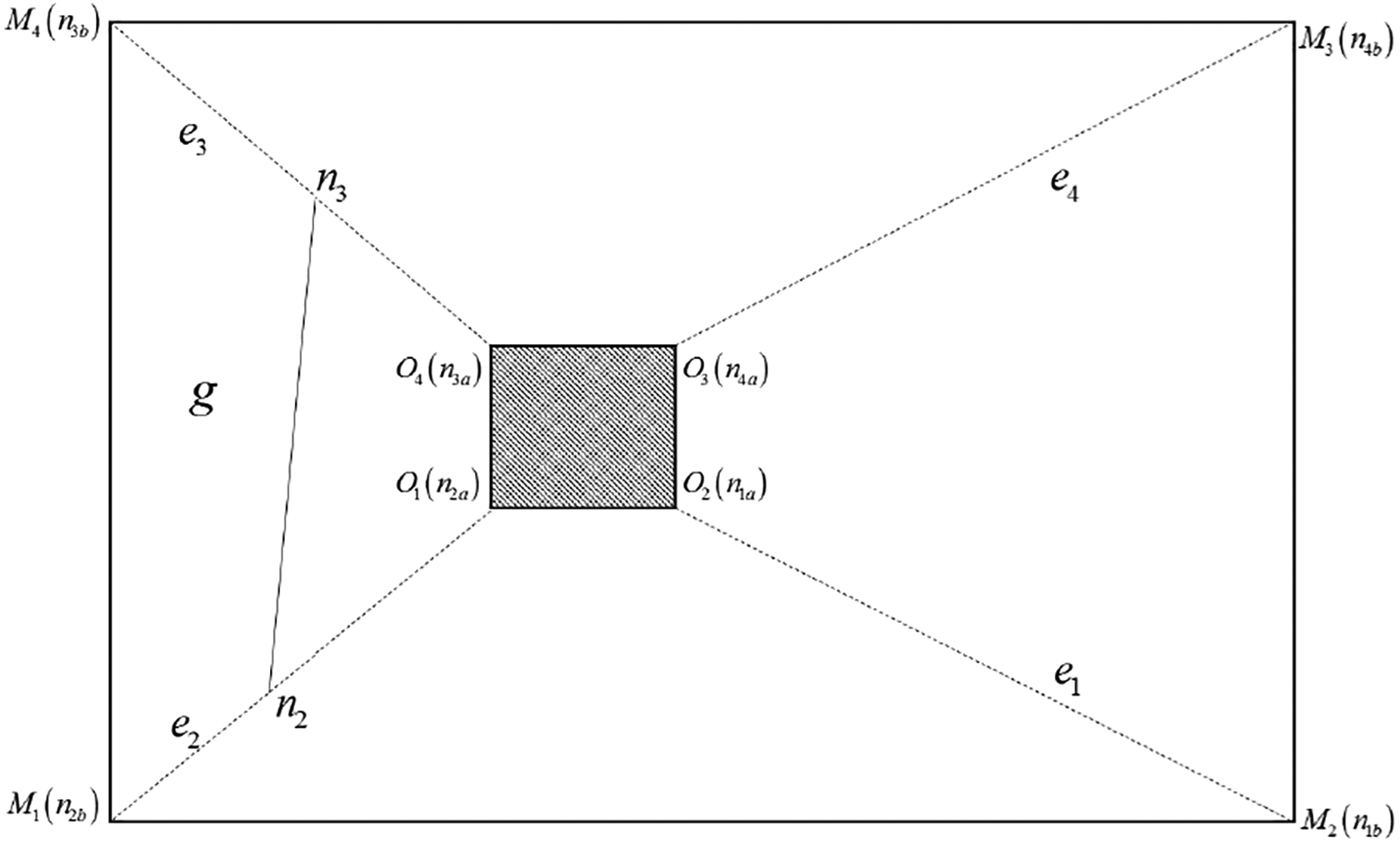
Select a node $n_{i} = n_{i a} + (n_{i b} - n_{i a}) α_{i}$ on each free link $e_{i} \in E$ , where $α_{i} \in [0, 1]$ , $n_{i a}$ and $n_{i b}$ are the two end points of the free link. Any two nodes n_n and n_m in the same free subspace g can be connected as a segment $n_{m n}$ of a feasible path. As Figure 1 shows, $M_{1} M_{2} M_{3} M_{4}$ and $O_{1} O_{2} O_{3} O_{4}$ are the map boundary and the obstacle boundary, respectively. $e_{1}, e_{2}, e_{3}, e_{4} \in E$ are four free links and n ₂ and n ₃ are two nodes in the same free subspace $g (n_{3 b} n_{3 a} n_{2 a} n_{2 b})$ .

Figure 1.

A feasible path in free subspace.

Several paths $p_{i} = \{x_{i n i t}, n_{i 1}, n_{i 2}, \dots, n_{i n}, x_{g o a l}\}$ from the start point to the end point can be obtained by connecting these nodes sequentially, where $n_{i j} (j = 1, \dots, n)$ is the $j th$ node of the $i th$ path. Two adjacent nodes on each path belong to the same free subspace g. For example, in Figure 2, $n_{11}$ and $n_{12}$ are the nodes on two free links which belong to the same free subspace g. Usually the parameter is set as $α_{i} = 1 / 2$ and a feasible path will be obtained under the above conditions, which means, the path p is the connection of the middle points of free links in a certain order. Then, the path p will be optimized with an optimization algorithm through adjusting parameter α. As Figure 2 shows, $p_{1} = \{x_{i n i t}, n_{11}, n_{12}, x_{g o a l}\}$ and $p_{2} = \{x_{i n i t}, n_{21}, n_{22}, x_{g o a l}\}$ are two different paths from $x_{i n i t}$ to $x_{g o a l}$ .

Figure 2.

A feasible path in free space.

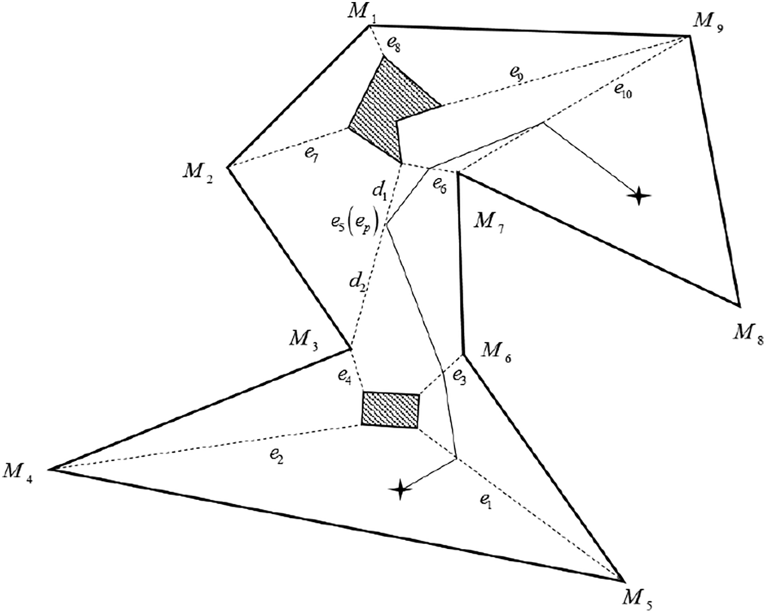
However, the result obtained by this method is not necessarily the optimal path. For example, as shown in the case of Figure 3, the DA algorithm will get the path $p_{1} = \{x_{i n i t}, n_{1}, n_{4}, x_{g o a l}\}$ . Then the path p ₁ can be optimized to get path $p_{2} = \{x_{i n i t}, O_{1}, O_{4}, x_{g o a l}\}$ . However, the optimal path is path $p_{4} = \{x_{i n i t}, O_{2}, O_{3}, x_{g o a l}\}$ which is optimized from path $p_{3} = \{x_{i n i t}, n_{2}, n_{3}, x_{g o a l}\}$ .

Figure 3.

A feasible path found by the traditional free space method.

From the above analysis, it can be seen that the traditional methods based on DA algorithm cannot guarantee that the global optimal path is in the selected connected domain and the optimization result can only be called local optimal path. Instead of using the DA algorithm to select connected domain and optimal algorithms to search the path, in this article a new map decomposition algorithm is designed to obtain multiple connected domains and each of them is composed of convex polygons. Then the ABC algorithm is used to search the optimal path in all the connected domains. The ABC algorithm will constantly search for new connected domain and discard the worse domains according to the searching results. It can guarantee that the result will not fall into a local minimum.

A new map decomposition method

The basic idea of the free space methods is to decompose the map into several free subspaces which are convex polygons. This article transforms the process of constructing free space into a problem of decomposing a concave polygon into several convex polygons. Firstly, we design a map decomposing algorithm for single-connected concave polygon (it stands for map without obstacle) based on the principle of concave polygon convex decomposition in the “Decomposition of single-connected concave polygon” section. Then, the algorithm for multi-connected concave polygon (it stands for map with obstacles) is proposed in the “Decomposition of multi-connected concave polygon” section. The multi-connected concave polygon can be converted into a single-connected concave polygon by excluding obstacles using virtual links. Thus, any map with obstacles can be decomposed into convex polygons.

Decomposition of single-connected concave polygon

Positive and negative determination of a polygon

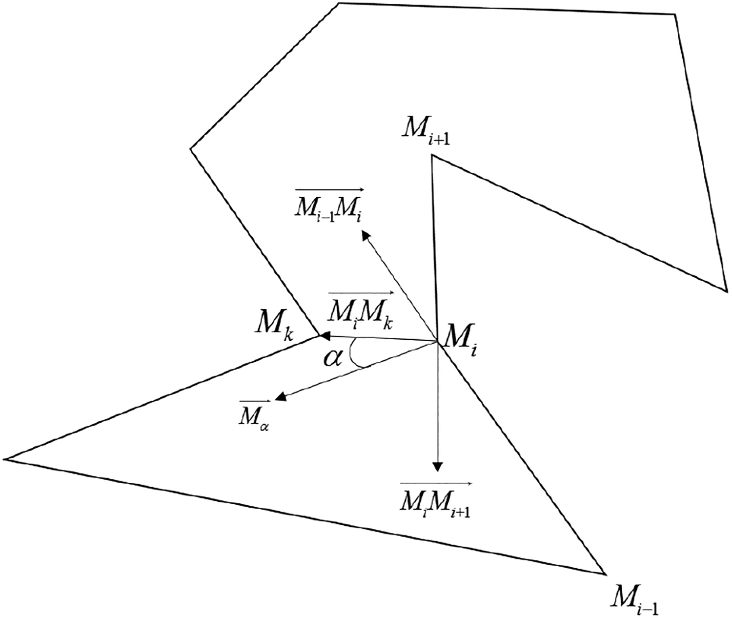
The positive or negative of a polygon refers to the order of the vertices of the polygon. A polygon is positive if the vertices are arranged counterclockwise, or negative if the vertices are arranged clockwise. The determining steps are as follows:

Find the convex vertices of the polygon M_i : the extreme point of the contour must be the convex vertex of the polygon.

Use convex vertices to determine whether the polygon is positive or negative: the two points adjacent to the convex vertex M_i are $M_{i - 1}$ and $M_{i + 1}$ , respectively, and the composed vectors are $\vec{M_{i - 1} M_{i}}$ and $\vec{M_{i} M_{i + 1}}$ .

If $\vec{M_{i - 1} M_{i}} \times \vec{M_{i} M_{i + 1}} > 0$ , the polygon is positive.

If $\vec{M_{i - 1} M_{i}} \times \vec{M_{i} M_{i + 1}} < 0$ , the polygon is negative.

Because three consecutive vertices of a polygon are not collinear, that $\vec{M_{i - 1} M_{i}} \times \vec{M_{i} M_{i + 1}} \neq 0$ . The above method of judging whether a polygon is positive or negative is shown in Figure 4.

Figure 4.

Positive and negative determination of a polygon.

The concave vertex of polygon

For a vertex M_i of a positive polygon, the two points that are adjacent to the vertex M_i are $M_{i - 1}$ and $M_{i + 1}$ . And the vectors composed of them are $\vec{M_{i - 1} M_{i}}$ and $\vec{M_{i} M_{i + 1}}$ .

If $\vec{M_{i - 1} M_{i}} \times \vec{M_{i} M_{i + 1}} > 0$ , the vertex M_i is a convex vertex.

If $\vec{M_{i - 1} M_{i}} \times \vec{M_{i} M_{i + 1}} < 0$ , the vertex M_i is a concave vertex.

Because three consecutive vertices of a polygon are not collinear, that $\vec{M_{i - 1} M_{i}} \times \vec{M_{i} M_{i + 1}} \neq 0$ . The above method of finding visible vertex is shown in Figure 5.

Figure 5.

The visible vertex.

The visible vertex

For a given vertex M_i of a polygon, its connection to any vertex M_j is $M_{i} M_{j}$ . If $M_{i} M_{j}$ is all inside or above the polygon, the vertex M_j is called the visible vertex of the vertex M_i .

For a given concave vertex M_i , the two points that are adjacent to the vertex are $M_{i - 1}$ and $M_{i + 1}$ and the composed vectors are $\vec{M_{i - 1} M_{i}}$ and $\vec{M_{i + 1} M_{i}}$ . The angle bisector of $\vec{M_{i - 1} M_{i}}$ and $\vec{M_{i + 1} M_{i}}$ is denoted as $\vec{M_{a}}$ . If the visible vertex is M_k , the vector of the visible vertex and the concave vertex is $\vec{M_{a} M_{k}}$ . α is the angle between $\vec{M_{a}}$ and $\vec{M_{i} M_{k}}$ , where $cos α = \frac{\vec{M_{a}} \cdot \vec{M_{a} M_{k}}}{|\vec{M_{a}}| \cdot |\vec{M_{a} M_{k}}|}$ . The smaller the α is, the better the visible vertex is.

Decomposition steps

Determine whether the polygon is positive or negative. If the polygon is positive, go to the next step. Otherwise, reverse the order of the vertices of the polygon.

Search for concave vertices starting from the first vertex. If there is no concave vertex, the polygon is a convex polygon. Otherwise go to the next step.

Select one of the concave vertices and search for the visible points of the concave vertex.

If there are concave vertices in the visible vertices, select the optimal visible vertices in the concave vertices. If there are no concave vertices in the visible vertices, the optimal visible vertex is selected among all visible vertices.

Connect the concave vertices and the optimal visible vertices. Decompose a polygon into multiple sub-polygons until all sub-polygons are convex polygons.

Decomposition of multi-connected concave polygon

Basic ideas and principles

According to the “Decomposition of single-connected concave polygon” section, any concave polygon without obstacle can be decomposed into several convex polygons. Here we consider a multi-connected concave polygon (map with obstacles). The main idea of this section is to convert a multi-connected concave polygon into a single-connected concave polygon. The most critical part is the introducing of virtual links which can exclude the obstacles from the original map and the left part of the map will be a single-connected concave polygon. Then the single-connected concave polygon can be decomposed into several convex polygons through the algorithm described in the “Decomposition of single-connected concave polygon” section.

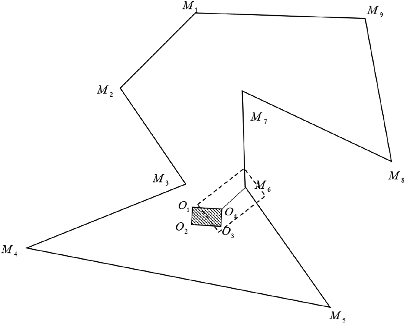
As Figure 6 shows, there is an obstacle $O_{1} O_{2} \dots O_{n}$ in the map $M_{1} M_{2} \dots M_{n}$ , and by connecting one of the vertices O_i of the obstacle with one of the vertices M_i of the map boundary, we can get a line and denote as $O_{i} M_{i}$ . Its vector can have two directions $\vec{O_{i} M_{i}}$ and $\vec{M_{i} O_{i}}$ . Assuming that there is a distance between the two vectors $\vec{O_{i} M_{i}}$ and $\vec{M_{i} O_{i}}$ and it is $Δ D \to 0$ , as shown in Figure 7. Connect the vertex O_i of obstacles to the vertex M_i of the map with these two vectors. Then the map becomes a single-connected domain polygon $M_{1} M_{2} \dots M_{i} O_{i} O_{i + 1} \dots O_{n} O_{1} \dots O_{i} M_{i} \dots M_{n}$ . If there are multiple polygon obstacles in the map, it is necessary to make sure that each obstacle is directly or indirectly connected with the vertex of the map boundary, as shown in Figure 8.

Figure 6.

A map with single obstacle.

Figure 7.

Local amplification of the link $O_{4} M_{6}$ .

Figure 8.

A map with multi-obstacle.

Converting steps

Given a set of map boundary vertices M_p , the set of obstacle polygons is $X_{o b s t a c l e}$ . Find all visible points in the map boundary vertex for each convex vertex in X and calculate the distance.

Connect a pair of vertices with the shortest distance. Insert the obstacle vertices sequence into the map boundary vertices sequence to form a new map boundary $M_{p n}$ . And remove the obstacle from the set of obstacles $X_{o b s t a c l e}$ .

If the set $X_{o b s t a c l e}$ is an empty set, the conversion from multiple connected domain map to single connected domain map is completed. Otherwise, return to step 1.

ABC algorithm

In the ABC algorithm, the colony of artificial bees contains three groups of bees: employed bees, onlooker bees, and scout bees. The scout bees are responsible for searching a new food source (global search). The employed bees can send the nectar information of the food sources to onlooker bees. The onlooker bees can evaluate the nectar information taken from all employed bees and choose a food source with a probability related to its nectar amount. Moreover, the employed bees and the onlooker bees can find a new food source in the neighborhood of the present one (neighborhood search). The employed bee whose food source has been abandoned becomes a scout.

Based on the above behavior of the bees, each cycle of the search consists of three steps for the ABC algorithm:

At the initialization stage, each half of the colony consists of the employed bees and the onlooker bees, respectively. A set of food source positions are randomly selected by the employed bees and their nectar amounts are determined. Each employed bee finds a new food source in the neighborhood of the present one and selects the better one.

At the second stage, the employed bees send the nectar information of the food sources to onlooker bees. Each onlooker bee chooses food source according to the nectar information (quality of the food source). As the nectar amount of a food source increases, the probability with which that food source is chosen by an onlooker increases, too.

At the third stage, after arriving at the selected area, each of the onlooker bees finds a new food source in the neighborhood of the present one and selects the better one. If a food source is not improved by a predetermined number of trials, then it will be abandoned by its employed bee or the employed bee is converted to a scout.

Each position of food source $X_{i} (i = 1, 2, \dots, S N)$ is a D-dimensional vector and can be represented as $X_{i} = [x_{i 1} x_{i 2} x_{i 3} \dots x_{i D}]$ .

An artificial onlooker bee chooses a food source depending on the probability value associated with that food source, p_i , which is calculated by the following expression

p_{i} = \frac{f i t_{i}}{\sum_{n = 1}^{S N} f i t_{n}}

where $f i t_{i}$ is the fitness value of the solution and SN is the number of solutions (food source positions). In ABC algorithm, the position of a food source represents a possible solution to the optimization problem and the nectar amount of a food source corresponds to the quality (fitness) of the associated solution.

In the ABC algorithm, while the exploration process carried out by artificial scouts is good for global optimization, the exploitation process managed by artificial onlookers and employed bees is very efficient for local optimization.

Karaboga and Basturk²⁹ compared the performance of the ABC with GA, PSO, and PS-EA by testing them on five high-dimensional numerical benchmark functions that have multimodality. They pointed out that the ABC algorithm has the ability to get out of a local minimum and can be efficiently used for multivariable, multimodal function optimization. Generally speaking, global searching methods such as ant colony algorithms and GAs can be used here. There are no restrictions on the use of global optimal algorithm for the proposed method. In this article, we give preference to ABC for its advantages in multimodal problems.

Path planning method

The path planning method proposed in this article mainly includes two parts:

Constructing a free space map.

Using the constructed free space and ABC algorithm to find the shortest path. The main structure is shown in algorithm 1.

Algorithm 1.

Body.

Algorithm 2 is a sub-function of algorithm 1. It is the process of constructing a free space by decomposing the map into free subspaces of several convex polygons. The meanings of the variables are given as follows:

Algorithm 2.

ConstructFreeSpace.

$X_{c o n v e x}$ and $X_{c o n c a v e}$ represent the set of convex polygon subspace and concave polygon subspace, respectively, where $X_{c o n v e x}, X_{c o n c a v e} \in X_{f r e e} = X / X_{o b s t a c l e}$ . Any concave polygon subspace in the concave polygon subspace set is denoted as $x_{c o n c a v e} \in X_{c o n c a v e}$ . $X_{p o l y g o n}$ is another form of X and both of them represent the entire map. $X_{p o l y g o n}$ represents the map by a polygon, but X represents the map by obstacles and map boundary. $e \in E$ represents the free links used to decompose the concave polygon. $x_{1}, x_{2} \in x_{c o n c a v e}$ represent two polygons obtained by decomposing a concave polygon with a free link.

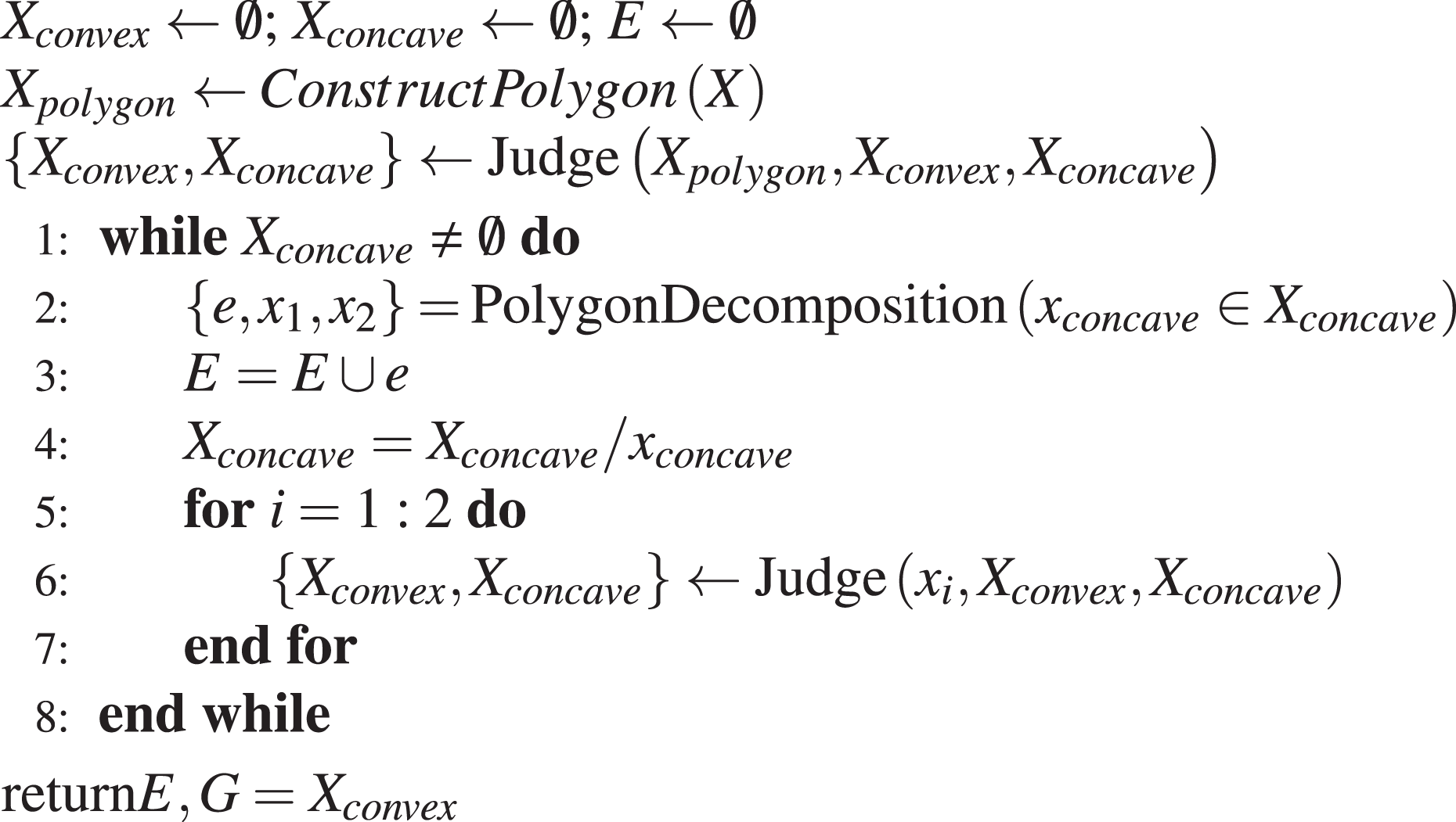
The function in algorithm 2 is introduced as follows:

ConstructPolygon: Construct a map with obstacles to a single-connected domain polygon. The method and steps are shown in the “Decomposition of multi-connected concave polygon” section.

Judge: Determine whether the polygon is a concave polygon or a convex polygon, and save it in the corresponding set.

PolygonDecomposition: Decompose a polygon into two polygons. The method and steps are shown in the “Decomposition of single-connected concave polygon” section.

Algorithm 3 is the ABC algorithm to find the shortest path.

Algorithm 3.

GeneratePath.

InitialPath (search the initial feasible path): Perform a global search to find a set of free links. Take the path nodes in the free links, and create an initial path by connecting them with the start point and the end point. The steps are as follows, and the illustration is shown in Figure 9:

Figure 9.

The illustration of how the initial path obtained.

Decompose the free area $X_{f r e e}$ of the map into several convex polygons. The free link is $e_{1}, e_{2}, \dots, e_{n}$ .

Determine the starting point and the target point to which the convex polygon $x_{p o l y g o n}^{s t a r t}$ and $x_{p o l y g o n}^{e n d}$ belongs. If $x_{p o l y g o n}^{s t a r t} = x_{p o l y g o n}^{e n d}$ , go to step 6. Otherwise, go to step 3.

Find all the free links that belong to $x_{p o l y g o n}^{s t a r t}$ and select a random one e_i . And save this free link into the set E.

Find another convex polygon $x_{p o l y g o n}^{n e x t}$ which e_i belongs. If $x_{p o l y g o n}^{n e x t} = x_{p o l y g o n}^{e n d}$ , go to step 6. Otherwise, randomly select a free link e_j that does not belong to set E among all the free links that belong to $x_{p o l y g o n}^{n e x t}$ .

Find another convex polygon $x_{p o l y g o n}^{n e x t}$ which e_j belongs. If $x_{p o l y g o n}^{n e x t} = x_{p o l y g o n}^{e n d}$ , go to step 6. Otherwise, randomly select a free link e_j that does not belong to set E among all the free links that belong to $x_{p o l y g o n}^{n e x t}$ . If e_j exists, store it in the set E, and repeat step 5. Otherwise, empty the set E and return to step 3.

Take a point on each free link in the set E, and connect them with the start and end points to generate the initial path.

Cost: Calculate the cost $b e n e f i t_{1}$ of the path $P_{i} = \{x_{i n i t}, p_{i 1}, p_{i 2}, \dots, p_{i n}, x_{g o a l}\}$ . The path cost in this article is the Euclidean distance of the path:

b e n e f i t_{1} = ‖p_{i 1} - x_{i n i t}‖ + ‖p_{i n} - x_{g o a l}‖ + \sum_{j = 1}^{n - 1} ‖p_{i (j + 1)} - p_{i j}‖

SearchTimes: Determine the times of each neighborhood search based on $b e n e f i t_{i}$ . The lower the path cost $b e n e f i t_{i}$ is, the larger the search time T_i is.

NeighbourhoodPath: This function is used to search for feasible paths in the neighborhood of the present one. In this method, the neighborhood search is defined as moving a certain path node on its own free link. The methods and steps are as follows:

Randomly select a free link e_p in set E. The path node on the free link is $P_{e p}$ , and the distances from the two end points $P_{e p 1}$ and $P_{e p 2}$ of e_p are d ₁ and d ₂, respectively. This step is shown in Figure 10.

Figure 10.

Random selection of free link e_p .

Randomly adjust the position of the path node $P_{e p}$ within a certain range: Move $P_{e p}$ to any end point $P_{e p i}$ of e_p by a random distance d, where $0 \leq d \leq a$ . If $r > d_{i}$ , $a = d_{i}$ . If $r \leq d_{i}$ , $a = r$ , where r is the setting adjustment range, $i = 1, 2$ . This step is shown in Figure 11.

Figure 11.

The neighborhood search of the path.

Results and discussion

Simulation of the proposed method

Usually obstacles in a map can be taken as simple polygons. A map with polygon obstacles, as shown in Figure 12, is taken for example to explain the method of this article. After convex decomposition, it can be seen that the map has been decomposed into several convex polygons and multiple connected domains can be obtained by composing different convex polygons. Figures 13 and 14 show two examples of the connected domain. There are many other connected domains in the map, which are not enumerated out one by one here. It means there will be different feasible paths in different connected domains. The simulation result of the proposed method is shown in Figure 12, the path is the shortest one. Figures 13 and 14 will be used to demonstrate the virtue of the proposed method in the next section while comparing with traditional free space methods.

Figure 12.

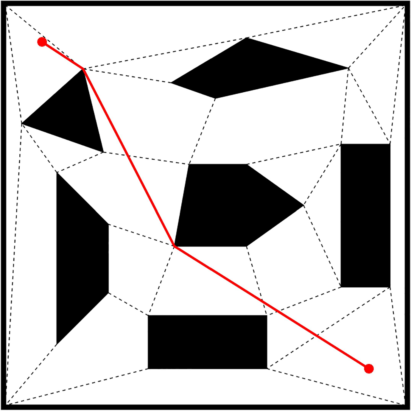
A map with simple multi-obstacle.

Figure 13.

Connected domain A.

Figure 14.

Connected domain B.

Besides the ordinary polygon obstacle cases, there are also some complex maps for path searching. From the simulation results of Qureshi and Ayaz,¹³ we can find that it is very difficult to get a feasible path in this kind of map as Figure 15 using classic methods or heuristic methods. This kind of map is usually a labyrinth or the target point surrounded by a continuous obstacle. It is easy to fall into local minimum and always takes a very long time to get a path. The proposed method has advantages in finding the shortest path easily and quickly. Take the map of Figure 15 for example, the searching time is about 1 s using the proposed method while about more than 10 s for the methods by Qureshi and Ayaz.¹³

Figure 15.

A map with complex obstacle.

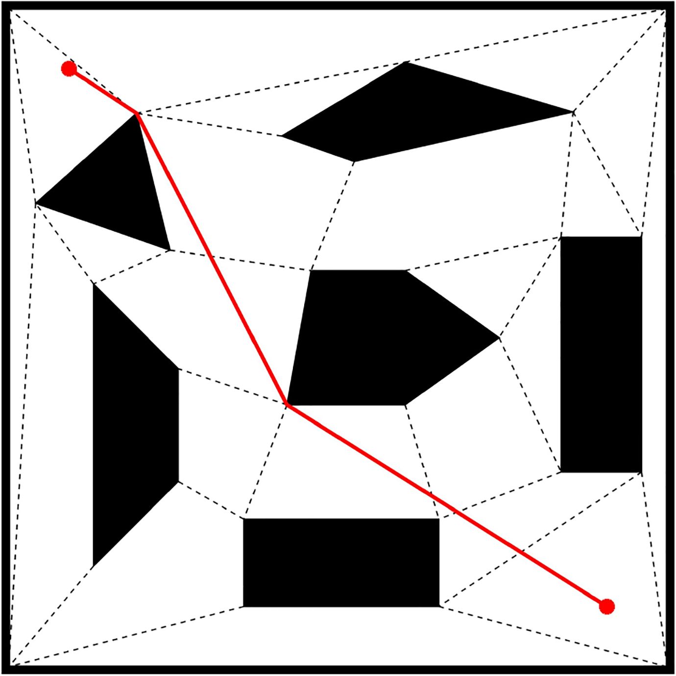
To prove the efficiency and the applicability of the proposed method, we consider the more complicated situation by adding both of the above obstacles to the map at the same time. The results are shown in Figure 16. It can be seen that it is the shortest path from the start point to the end point. And the searching time is also about 1 s.

Figure 16.

A map with combination obstacles.

Parameter sensitivity analysis

There are several important parameters of the ABC algorithm such as the maximum global search times $T_{limit}$ , the maximum neighborhood search times $T_{max}$ , and the number of employed bees N. These parameters have a great influence on the results. Here we will analyze the impact of these parameters based on a large number of simulation data.

To conduct the analysis, we will adjust one parameter at a time while the others are fixed. First, it is found that in the case of the above map in Figure 16, the path quality is high when the number of employed bees N is 3–5, and the planning process takes a short time. So the number of employed bees N is set to 3. Then, the maximum global search times $T_{limit}$ is analyzed as an independent variable to find the trend of path length and planning time. For each value of $T_{max}$ , we conduct 500 times of simulation and obtain the average path lengths. The results are shown in Figure 17. It can be seen that the average path length decreases as the maximum global search times $T_{limit}$ increases. The rate of decrease gradually slows down, and the average path length gradually approaches the theoretical shortest path length.

Figure 17.

Average path length for different $T_{max}$ .

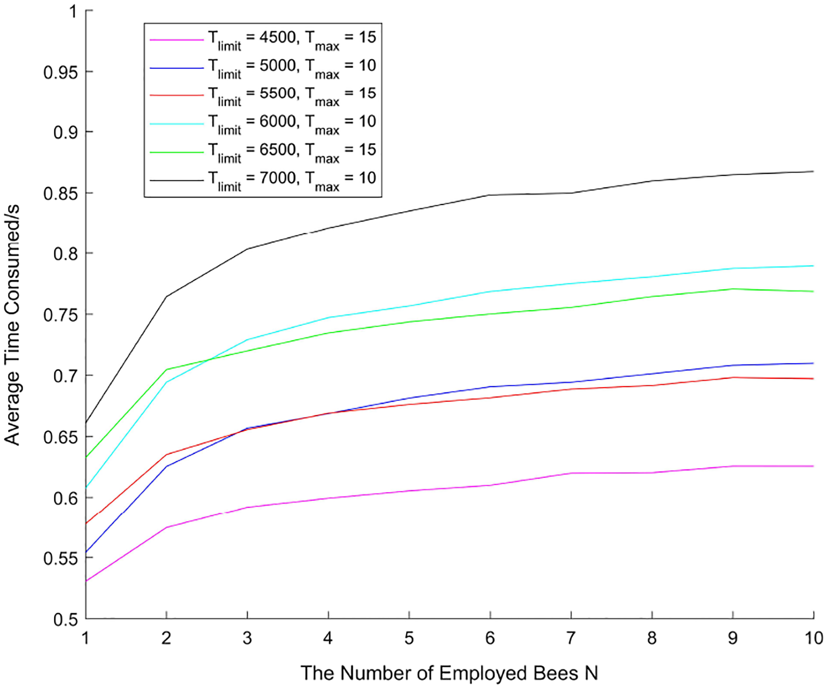
Also, we can get the average time consumption as shown in Figure 18. It can be seen that the average planning time increases while the maximum global search times $T_{limit}$ increases.

Figure 18.

Average time consumption for different $T_{max}$ .

The impacts of the maximum global search times $T_{limit}$ and the maximum neighborhood search times $T_{max}$ on path length and time consumption are also calculated as shown in Figures 19 and 20. The standard deviations of the path length and planning time are given.

Figure 19.

Standard deviation of path length.

Figure 20.

Standard deviation of time consumption.

From the statistical results in Figures 19 and 20, it can be seen that when the maximum neighborhood search times $T_{max}$ is around 10, we can get shorter path length while using less planning time. When the maximum neighborhood search times $T_{max}$ is 5–15 and the maximum global search time $T_{limit}$ is more than 4500, the average path length decreases, the path quality becomes better, and also the path length and the path planning time tend to converge.

Based on the above results, the influence of employed bees number N on the length of path and time consumption is analyzed under the following conditions: (1) $T_{limit} = 4500$ , $T_{max} = 15$ ; (2) $T_{limit} = 5000$ , $T_{max} = 10$ ; (3) $T_{limit} = 5500$ , $T_{max} = 15$ ; (4) $T_{limit} = 6000$ , $T_{max} = 10$ ; (5) $T_{limit} = 6500$ , $T_{max} = 15$ ; (6) $T_{limit} = 7000$ , $T_{max} = 10$ .

As shown in Figures 21 and 22, when the number of employed bees N changes from 1 to 2, the average path length drops sharply. However, when the number of employed bees N gradually increases, the average path length does not change significantly. With the increase of the number of employed bees N, the average planning time gradually increases, but the increasing rate gradually decreases, and the planning time tends to converge.

Figure 21.

Average path length for different parameters.

Figure 22.

Average time consumption for different parameters.

From the above simulation results of this section, it can be seen that the proposed method can get a high-quality path in a short time by choosing appropriate parameters. The simulation time is usually within 1 s.

Comparison with the other free space method

DA was widely used in the free space methods to find the connected domain from the starting point to the end point.^{16,22

–28}. In DA-based methods, usually the midpoints of two free links are connected and the length of the connected line is set as the weight to choose the better connected domain. Then, the shortest path from the starting point to the end point will be searched in the chosen connected domain by using optimization algorithms. Local minimum path can be found in the connected domain, but the global shortest path may not be in the selected connected domain.

Here we still take the map of Figure 12 for example. The shadow parts in Figures 23 and 25 present two different connected domains, and the length of the line from the start point to the end point is the weight of the connected domain. The connected domain in Figure 23 is better than the one in Figure 25 for it has less weight. Thus the domain in Figure 23 will be selected and the DA-based method searches the shortest path in it. The line in Figure 24 is the local shortest path found by DA-based method.

Figure 23.

The weight of connected domain A.

Figure 24.

The shortest path in connected domain of Figure 23.

Figure 25.

The weight of connected domain B.

However, the global shortest path in this map is actually in the connected domain of Figure 25. The path shown in Figure 26 is the global shortest one which is obtained by the method proposed in this article. It is shorter than the one in Figure 24. The using of the bee colony algorithm can help searching multiple connected domains and avoid falling into the local solution.

Figure 26.

The shortest path in connected domain of Figure 25.

Comparison with RRT* algorithm

For the map of Figure 12, the performances of RRT* and the proposed method are compared based on a great number of simulations. One thousand simulations have been conducted for different values of global maximum search times $T_{limit}$ and 1000 simulations for different branch length d of search tree in RRT*. r is the other parameter of RRT*. The average search time and average path length for each 1000 simulations have been obtained and shown in Table 1. For the proposed method, it can be seen that the larger the $T_{limit}$ is, the longer the path planning time is, and the shorter the average path length is. Compared with RRT*, the path length obtained by the proposed method is much shorter when $T_{limit}$ is bigger than 25,000 and the path planning time does not significantly increase. For this kind of simple maps, the proposed method does not show many advantages in time consumption, but it can get better path. Figure 27 shows one of the feasible paths found by RRT* algorithm.

Figure 27.

The result of RRT* algorithm for simple-obstacle map. RRT*: rapidly exploring random tree star.

Table 1.

Comparison with RRT* for simple-obstacle map.

The proposed method
$T_{limit}$	$T_{max}$	Time	Length of path
15,000	15	0.9494 s	626.5595
25,000	15	1.7585 s	602.8108
50,000	15	3.0317 s	592.2346
RRT* algorithm
d	r	Time	Length of path
20	40	0.5630 s	650.7118
15	45	0.9594 s	631.9194
25	75	0.4505 s	619.5313

RRT*: rapidly exploring random tree star.

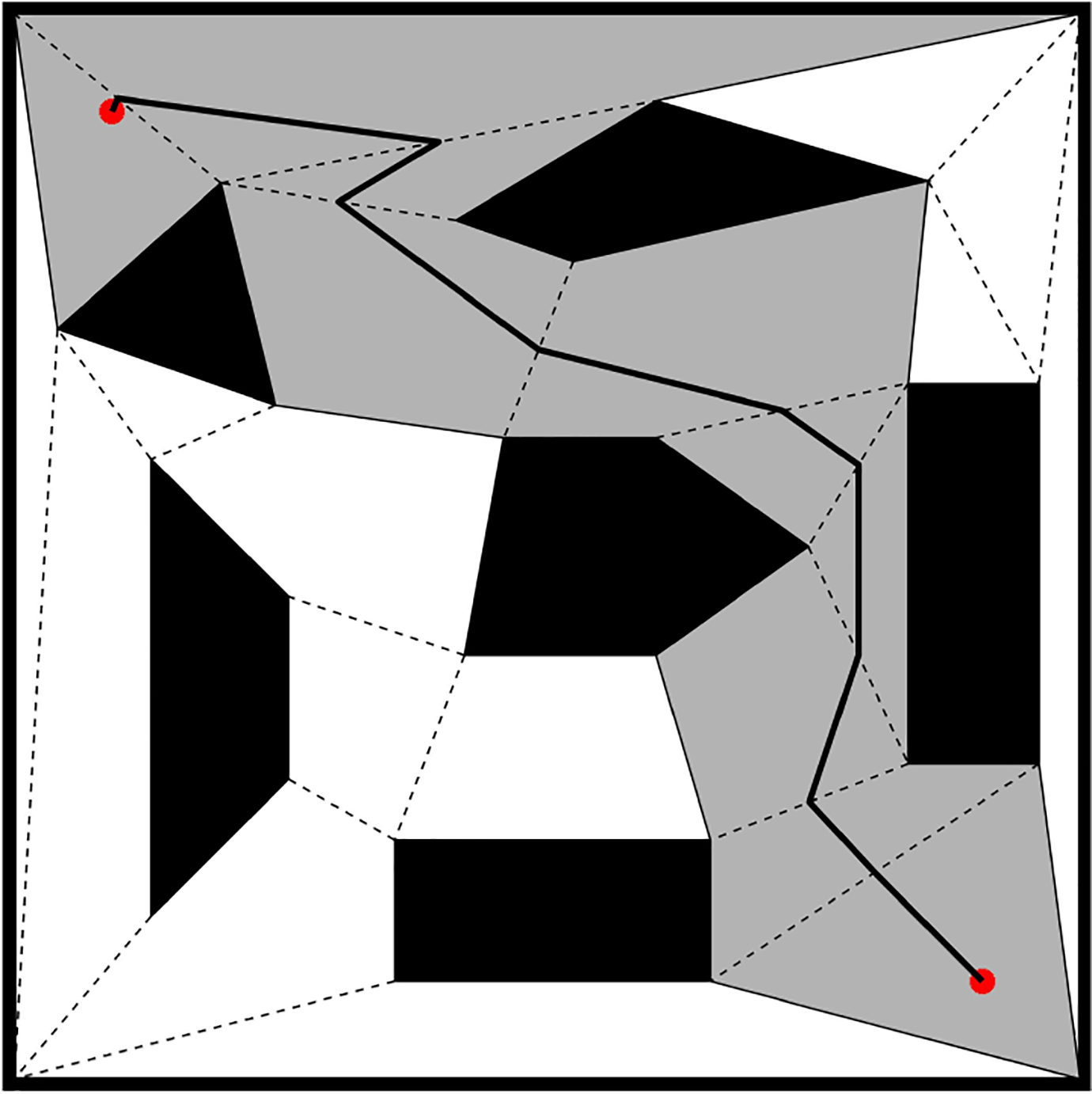
Then we take a complex map for example to show the advantages of the proposed method. In this map, obstacles are no longer independent simple convex polygons, but are irregular obstacles which increase difficulties for path planning. The two methods are simulated under different groups of parameters. Each group is simulated for 1000 times and the average planning time and average path length are shown in Table 2. The proposed method can get better paths while the planning time is much shorter than RRT*. Figures 28 and 29 show the results obtained by the proposed method and RRT*.

Table 2.

Comparison with RRT* for complex-obstacle map.

The proposed method
$T_{limit}$	$T_{max}$	Time	Length of path
2000	15	0.1160 s	749.0245
5000	15	0.2892 s	727.2539
10,000	15	0.6865 s	726.0352
RRT* algorithm
d	r	Time	Length of path
20	60	38.8282 s	756.1831
20	80	36.1654 s	774.8951
30	120	15.5060 s	796.9362

RRT*: rapidly exploring random tree star.

Figure 28.

The result of the proposed method for complex-obstacle map.

Figure 29.

The result of RRT* algorithm for complex-obstacle map. RRT*: rapidly exploring random tree star.

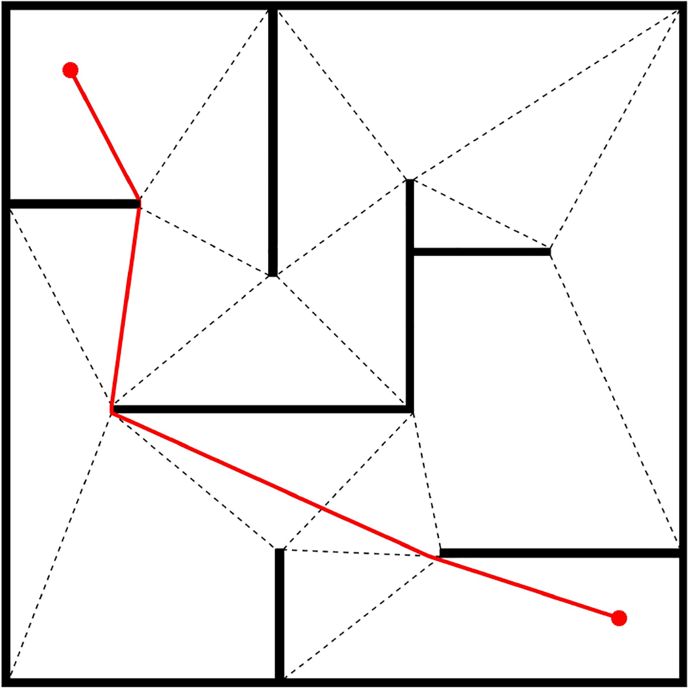
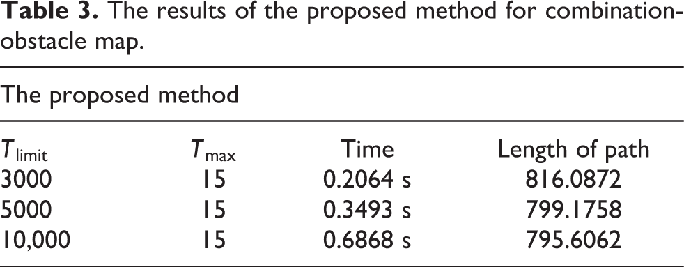
However, for the maps shown in Figures 15 and 16, which are even more complex than Figures 12 and 28 as there is labyrinth obstacle in it, the proposed method has more advantages than RRT*. Here also 1000 simulations have been conducted for each different parameter to find shortest path in Figure 16. RRT* algorithm cannot find a feasible path in a very long time (about 1 min), but the proposed method can still find the shortest path in a short time (about 1 s). The results are shown in Table 3.

Table 3.

The results of the proposed method for combination-obstacle map.

The proposed method
$T_{limit}$	$T_{max}$	Time	Length of path
3000	15	0.2064 s	816.0872
5000	15	0.3493 s	799.1758
10,000	15	0.6868 s	795.6062

Application

The proposed method can be applied on the situation of urban environment and field environment, for both mobile robot and UAV. It is especially efficient for planar mobile robot in the urban environment since the maps are easier to simplify. An example is given to show the application in urban environment.

Figure 30 is a satellite map. We need to find a shortest path from A to B. The buildings in the map are taken as obstacles. First these obstacles are simplified as polygons by defining their boundaries (black lines as shown in Figure 31). Then the problem is turned to search path from A to B avoiding these obstacles. The red line shown in Figure 31 is the result obtained by the proposed method.

Figure 30.

The satellite map.

Figure 31.

The result of proposed method for satellite map.

To further illustrate the application scenario of this method, the following satellite map of the sea surface is taken. The method is applied for ship route planning between A and B. First the coastline has been redrawn in straight lines and the boundary is determined (the black thick lines in the figure). Then the islands are taken as obstacles presented by black thin lines. The original satellite map now becomes a polygon map. The shortest route from A to B can be obtained by the proposed method (as the red line shown in Figure 32).

Figure 32.

The result of proposed method for another satellite map.

Based on the above two examples, it can be seen that the proposed method can be applied in many different scenarios. It has short time consumption even for complex maps such as narrow or labyrinth terrain. Unlike Shiller,¹⁷ Savkin and Hoy,¹⁸ and Liu and Arimoto,¹⁹ to apply the method, the obstacles in the map and the map boundaries should be treated as polygons first. The polygonization of map may cause small loss of accuracy for some irregular maps, but it is still acceptable. For most cases, the proposed method can find the optimal path with high accuracy and short time consumption.

As the development of robot technique, path planning technology in future will be widely applied in robot field such as multi-robot collaboration, complex environment, multi-dimensional environment, and so on. Also the characteristics of robot should be taken into account for more application scenario such as bionic robot, space robot, and other under-actuated robotics.³⁰ The robot ability of path tracking should be considered when planning a feasible path. Furthermore, real-time planning should be considered for unknown environment such as in the study of Shiller¹⁷ and Savkin and Hoy,¹⁸ and the proposed method needs to be improved based on the information obtained by detection sensors.

Conclusions

This article presents a new path planning method based on concave polygon convex decomposition and ABC algorithm. Several simulation and comparison with other methods are carried out. The results show that the proposed method has high computational efficiency in providing the optimal path due to its high efficiency in segmenting the map and the multi-domain searching. Compared with the traditional free space methods and RRT*, it is more able to find the global optimal path with efficiency and rapidity, especially for complex maps. Also, numerical sensitivity analysis on critical parameters is done. It is found that the maximum neighborhood search times, $T_{max}$ , and the number of employed bees, N, are the most important parameters for path searching. The suggested values are 15–20 for $T_{max}$ and 3–5 for N. If these two parameters are determined, the greater the maximum global search times $T_{limit}$ is, the better the path quality is and the shorter the search time is. The path quality and search time will significantly improve if the maximum global search times, $T_{limit}$ , comes close to a specified value.

Algorithm 4.

NeighbourhoodSearch.

Footnotes

Declaration of conflicting interests

The author(s) declared no potential conflicts of interest with respect to the research, authorship, and/or publication of this article.

Funding

The author(s) received no financial support for the research, authorship, and/or publication of this article.

ORCID iD

Zhaoying Li

References

Raja

Pugazhenthi

. Optimal path planning of mobile robots: a review. Int J Phys Sci 2012; 7(9): 1314–1320.

Elbanhawi

Simic

. Sampling-based robot motion planning: a review. IEEE Access 2014; 2: 56–77.

Wang

Zhu

Wang

, et al. An improved artificial potential field method of trajectory planning and obstacle avoidance for redundant manipulators. Int J Adv Robot Syst 2018; 15(5): 1–13.

Luo

Mei

, et al. UAV path planning in mixed-obstacle environment via artificial potential field method improved by additional control force. Asian J Control 2015; 17(5): 1600–1610.

Long

Gong

Dai

, et al. Mobile robot path planning based on ant colony algorithm with A* heuristic method. Front Neurorobot 2019; 13: 15.

Nemec

Gregor

Bubenková

, et al. Improving the hybrid A* method for a non-holonomic wheeled robot. Int J Adv Robot Syst 2019; 16(1): 1–12.

Setiawan

Pratama

Sang

, et al. Experimental comparison of A* and D* lite path planning algorithms for differential drive automated guided vehicle. Lect Notes Electr Eng 2014; 282: 555–564.

Yan

Liu

Xiao

. Path planning in complex 3D environments using a probabilistic roadmap method. Int J Auto Comput 2013; 10(6): 525–533.

Karaman

Frazzoli

. Incremental sampling-based algorithms for optimal motion planning. arXiv preprint arXiv:1005.0416 , 2010.

10.

Karaman

Frazzoli

. Sampling-based algorithms for optimal motion planning. Int J Robot Res 2011; 30(7): 846–894.

11.

Véras

LGDO

Medeiros

FLL

Guimarães

LNF

. Rapidly exploring random tree* with a sampling method based on Sukharev grids and convex vertices of safety hulls of obstacles. Int J Adv Robot Syst 2019; 16(1): 1–19.

12.

Jeong

Lee

Kim

. Quick-RRT*: triangular inequality-based implementation of RRT* with improved initial solution and convergence rate. Expert Syst Appl 2019; 123: 82–90.

13.

Qureshi

Ayaz

. Potential functions based sampling heuristic for optimal path planning. Auton Robot 2016; 40(6): 1079–1093.

14.

Xiong

Chen

, et al. Path planning of multiple autonomous marine vehicles for adaptive sampling using Voronoi-based ant colony optimization. Robot Auton Syst 2019; 115: 90–103.

15.

Garrido

Moreno

Abderrahim

, et al. Path planning for mobile robot navigation using Voronoi diagram and fast marching. In: 2006 IEEE/RSJ international conference on intelligent robots and systems, Beijing, China, 9–15 October 2006, pp. 2376–2381. IEEE.

16.

Eslami

. A real-time global optimal path planning for mobile robot in dynamic environment based on artificial immune approach. GSTF J Comput (JoC) 2018; 2(1): 104–109.

17.

Shiller

. Online suboptimal obstacle avoidance. Int J Robot Res 2000; 19(5): 480–497.

18.

Savkin

Hoy

. Reactive and the shortest path navigation of a wheeled mobile robot in cluttered environments. Robotica 2013; 31(2): 323–330.

19.

Liu

Arimoto

. Path planning using a tangent graph for mobile robots among polygonal and curved obstacles. Int J Robot Res 1992: 4(4): 376–382.

20.

Kloetzer

Mahulea

Gonzalez

. Optimizing cell decomposition path planning for mobile robots using different metrics. In: 19th international conference on system theory, control and computing (ICSTCC), Cheile Gradistei, Romania, 14–16 October 2015, pp. 565–570. IEEE.

21.

Chatila

. Path planning and environment learning in a mobile robot system. In: Proceedings of the 5th European conference on artificial intelligence, Orsay, France, 1–3 July 1982, pp. 211–215. ACM.

22.

Habib

Asama

.Efficient method to generate collision free paths for an autonomous mobile robot based on new free space structuring approach. In: Proceedings IROS’91: IEEE/RSJ international workshop on intelligent robots and systems’91, Osaka, Japan, 3–5 November 1991, pp. 563–567. IEEE.

23.

Yang

Gao

Luo

.An improved ant colony system algorithm for optimal path planning problem of mobile robots. In: 2010 second international conference on computer modeling and simulation, vol. 1, Sanya, Hainan, China, 22–24 January 2010, pp. 526–530. IEEE.

24.

Guan-Zheng

TAN

Huan

Sloman

. Ant colony system algorithm for real-time globally optimal path planning of mobile robots. Acta Automatica Sinica 2007; 33(3): 279–285.

25.

Kang

Lee

Kim

.Path planning algorithm using the particle swarm optimization and the improved Dijkstra algorithm. In: 2008 IEEE Pacific-Asia workshop on computational intelligence and industrial application, vol. 2, Wuhan, China, 19–20 December 2008, pp. 1002–1004. IEEE.

26.

Liang

.Global path planning for mobile robot based genetic algorithm and modified simulated annealing algorithm. In: Proceedings of the first ACM/SIGEVO summit on genetic and evolutionary computation, Shanghai, China, 12–14 June 2009, pp. 303–308. ACM.

27.

Shen

Yuan

. A novel poly-clone particle swarm optimization algorithm and its application in mobile robot path planning. In: 2010 Chinese control and decision conference, Xuzhou, China, 26–28 May 2010, pp. 2271–2276. IEEE.

28.

Hao

Shen

Zhao

.Path planning for aircraft based on MAKLINK graph theory and multi colony ant algorithm. In: 2009 international joint conference on computational sciences and optimization, vol. 2, Sanya, Hainan, China, 24–26 April 2009, pp. 232–235. IEEE.

29.

Karaboga

Basturk

. A powerful and efficient algorithm for numerical function optimization: artificial bee colony (ABC) algorithm. J Global Optim 2007; 39(3): 459–471.

30.

Wang

Liu

. Underactuated robotics: a review. Int J Adv Robot Syst 2019; 16(4): 1–29.

A new path planning method based on concave polygon convex decomposition and artificial bee colony algorithm

Abstract

Keywords

Introduction

Preliminary material of free space method

A new map decomposition method

Decomposition of single-connected concave polygon

Positive and negative determination of a polygon

The concave vertex of polygon

The visible vertex

Decomposition steps

Decomposition of multi-connected concave polygon

Basic ideas and principles

Converting steps

ABC algorithm

Path planning method

Results and discussion

Simulation of the proposed method

Parameter sensitivity analysis

Comparison with the other free space method

Comparison with RRT* algorithm

Application

Conclusions

Footnotes

Declaration of conflicting interests

Funding

ORCID iD

References