Sage Journals: Discover world-class research

Abstract

Leg stiffness plays a critical role in legged robots’ speed regulation. However, the analytic solutions to the differential equations of the stance phase do not exist, of course not for the exact analytical solution of stiffness. In view of the challenge in dealing with every circumstance by numerical methods, which have been adopted to tabulate approximate answers, the “harmonic motion model” was used as approximation of the stance phase. However, the wide range leg sweep angles and small fluctuations of the “center of mass” in fast movement were overlooked. In this article, we raise a “triangle motion model” with uniform forward speed, symmetric movement, and straight-line center of mass trajectory. The characters are then shifted to a quadratic equation by Taylor expansion and obtain an approximate analytical solution. Both the numerical simulation and ADAMS-Matlab co-simulation of the control system show the accuracy of the triangle motion model method in predicting leg stiffness even in the ultra-high-speed case, and it is also adaptable to low-speed cases. The study illuminates the relationship between leg stiffness and speed, and the approximation model of the planar spring–mass system may serve as an analytical tool for leg stiffness estimation in high-speed locomotion.

Keywords

High-speed locomotion stiffness stance time analytical approximation SLIP

Introduction

The research on robot’s high-speed movement and operation^1

–4 is a significant topic, especially for legged robots, which could be used as an all-terrain platform in various missions.⁵ In 1899, Muybridge used stop-motion photography to document animals’ locomotion, such as cats, dogs, camels, and horses.⁶ Based on a large number of experimental biological data, researchers have summarized a spring-loaded inverted pendulum (SLIP)⁷ model to describe the nature of animals’ dynamic motion, among which, spring represents the mechanical properties of animal tissues, such as bones, muscles, tendons, and ligaments. The SLIP model has become the most widely used model of legged robots in dynamic running. In this model, the centralized mass of the body and the stiffness of the legs have a decisive influence on energy storage and efficiency.⁸ Based on the spring–mass model, Raibert and Tello had successfully developed a control scheme for legged robots from monopod to quadruped.⁹ The iSprawl used tuned axial stiffness in conjunction with feed-forward position profiles of the prismatic leg.¹⁰ The MIT Cheetah demonstrated a stable trot via the stiffness control of the stance legs.¹¹ These studies confirm the importance of “leg stiffness” on locomotion behaviors. Legged robots’ high-speed locomotion is one of the challenging issues in robotic research.^11

–14 However, few studies covered the qualitative change of leg stiffness with the running speed increasing.

The use of mechanical impedance to control legged robots has been motivated by animals of different sizes and leg layouts using spring-like interactions with the ground.^15

–19 Many previous evidence have indicated that leg stiffness is independent of the forward speed, the stiffness of the leg (K _leg) changes slightly with speed in all observed animals (dogs, goats, horses, and kangaroos with a speed under 5 m/s),^15,20,21 while other researchers reported a positive correlation between running speed and leg stiffness.^22

–26 The deviation comes from the different applied velocity, different leg sweeping angle, and the measurement accuracy. Animals are generally inclined to develop a lower leg stiffness if a larger sweep angle is available to support the velocity increment.²⁴ Without significant changes in leg stiffness, a relatively stable unit-transportation-energy-consumption (COT) is achieved when speed increased gradually.^21,27 However, the greatest touchdown angle by the leg spring during the ground contact phase was almost the same (around 28°) in animals of various body sizes,¹⁵ indicating that all locomotion is restricted by the friction cone from increasing the sweep angle infinitely.

In 1990, a unique concept of “vertical leg stiffness” (K _vert) was raised by McMahon and Cheng to embrace the multivariables in running and it was quoted in many research works.^15,24,25,28 The coupling mechanics show that the leg stiffness increases linearly and slowly with the horizontal velocity, while K _vert presents a significantly quadratic exponential growth when the other parameters remain unchanged. K _vert describes the vertical motion of the center of mass (COM) during the ground contact time and is essential in determining how long the spring–mass system remains on the ground.²⁵ The vertical stiffness could be calculated by leg compression length and ground reaction force (GRF) (Figure 1(a)), where the maximum GRF can be measured by the force sensors installed on the feet/floor or by methods from TH Witte.²⁹ K _vert is valuable in estimating the critical parameter, Stance Time.³⁰ Since seeking the exact analytical solution of the motion during stance remains unsettled due to the nonintegral terms contained in the nonlinear dynamic equations, a common approach to tackle it is to simply the equations,^{15,25,31

–34} resulting in an approximate solution of the state parameters. A mass–spring oscillator in the vertical direction was the most commonly used model to calculate the stance time as the gravitational force is ignored compared with the initial reaction force. In this article, we call this approximate model “harmonic motion model” (HMM)¹⁵. Under the approximation, the system will remain in contact with the ground for half of a resonant period of vertical vibration which is positively correlated with the reciprocal of K _vert, and K _vert is equal to K _leg when hopping vertically.¹⁵

Figure 1.

Concept of the ‘Vertical stiffness’ and the ‘Triangle motion model’ in SLIP: (a) The ‘Vertical stiffness’ relies on the compression under the line between touchdown and liftoff and (b) the ‘triangle motion model’ assumes that the trajectory of the center of mass is a straight line. SLIP: spring-loaded inverted pendulum.

Nonetheless, the current definition of “vertical stiffness” still retains some ambiguities since it is difficult to distinguish the vertical displacement change which is caused by the tilting of the inverted pendulum or by the spring compression (view Figure 1(a)). In extreme cases, when an uncompressible inverted pendulum touches down with angle θ and is pushed up to the vertical position by inertia force, it will produce a negative △y, and △l equals to zero. Another case is that when the leg spring is hard enough, the compression of the leg in the vertical direction may be close to zero, which makes it difficult to calculate the actual value of △y. Therefore, it is hard to use the theory to estimate the stance time. In some instances of small leg sweep angle, researchers would use leg stiffness to replace vertical stiffness, and use the stance time of hopping in place to replace that with initial horizontal velocity and modify it step by step in the feedback process.⁹ Since the Stance Time plays a key role in bridging stiffness selection and touchdown angle preparation on the premise of symmetric movement and neutral point theory, a more precise analytical equation of the stance time was adopted by taking gravity into account in McMahon and Chen’s paper.^25,31,32

For the high-forward-velocity robots, more accurate analytical models were introduced. Geyer et al. derived analytical solutions to the stance map of the energy conservative SLIP model on symmetric stride. It was assumed that the sweep angle Δθ and the spring compression Δl during stance are sufficiently small (approach to zero).³³ These remarkable assumptions guarantee the success of the approximating process. Similar assumptions were also used in Haitao Yu’s regular perturbation method,³⁴ and both of them derived straightforward expansion solutions with high predicted precision. However, the approximations lose accuracy rapidly with an angular velocity at touchdown and radial spring compression rate increased, which are the classic characters of high-speed running.

With both the conciseness and accuracy in mind, and after extensive numerical simulations, a numerical fitting approach was taken to describe the relation between stance time and velocity. Then a modified stiffness with speed-related quadratic growth was applied to calculate the stance time.³² Other empirical fitting formulas of stiffness from experiments were also accessible.²⁵ However, the diversity of the actual robot system makes it laborious to fit the stiffness curve without pre-verified data under specific boundary conditions.

To sum up, accurate knowledge of leg stiffness is important as it is the basis for stabilizing control. It may lead to rapid failure in ultra-high-speed dynamic running if sustained errors are accumulated.³¹ Although these studies have demonstrated the effectiveness of stiffness increment in high-speed running, yet almost none of them reported a rapid-response analytical approach for stiffness to handle the ultra-short contact phase.³⁵ A better estimation of stiffness is required to avoid the wide range errors of the touchdown point as well as inadequate utilization of leg sweep angle. This work aims to pursue an accurate approximation of stance map validity in high-speed locomotion. The study illuminates the relationship between leg stiffness and speed, and the approximation model of the planar spring–mass system may serve as an analytical tool for estimating leg stiffness in high-speed locomotion, which is beneficial for making full use of the leg sweep angle and maintaining stability.

The remainder of this article is structured as follows: In the second section, the concise modeling of the SLIP while in high-speed locomotion is formulated in the “Problem formulation,” meanwhile a kind of “triangle motion model” (TMM) containing the simplest high-speed features is proposed. In the third section, the simplified solution of the stance phase is obtained by TMM and the stiffness strategy is introduced. In the fourth section, the method accuracy is analyzed by comparing the results between different analytical approaches and the results of numerical simulations. Multi-body dynamic simulations in ADAMS platform are outlined to consider the disturbance in the actual physical system and verify the theory. In the fifth section, limited conditions associated with incremental stiffness and the suitable range of the model are discussed. Finally, the sixth section presents the conclusion.

Problem formulation

As depicted in Figure 1(b), the conservative system consists of a point mass m and a massless prismatic leg connected to the hip with Hooke’s law. The spring–mass system lands on the ground with an initial touchdown angle θ ₀, forward velocity u, and downward velocity v_y ₀. The velocity u takes the forward direction of bounce as positive and v_y ₀ is positive if it takes a vertical upward direction. The alternative touchdown and liftoff events contribute to the switching between the stance and flight phase. It is a passive model with no torque applied at the hip or active thrust in the elastic leg during the contact. The foothold keeps stationary without slipping. The system reaches the bottom as the vertical velocity decreases to zero. If the foothold falls on the “neutral point,” the trajectory of the COM will be symmetrical along the vertical line with a uniform touchdown and liftoff angle, and the forward velocity between the moment of touchdown and liftoff will be equal, while the symbol of the vertical velocity is reversed.

The incident point is taken as the origin of the horizontal motion. On the left side of the vertical line, the angle between the spring leg and the vertical line is negative, and on the right side of the vertical line, the angle is positive. As in high-speed locomotion, the touchdown angle is always swept to its maximum, which is represented as θ ₀. If the friction coefficient between the toe and the ground is represented by f, then the angle θ ₀ will be defined as a scalar that $θ_{0} \in [0 °, arctan (f))$ .

As mentioned above, leg stiffness acts as a critical bridge in speed regulation which determines the stance time and influences the leg sweep angle. The following equation describes the motion of the SLIP model in the vertical direction during the stance phase. It can be organized into a differential form

m a_{y} = K_{leg} Δ l cos θ - m g

\ddot{y} + ω^{2} y = ω^{2} l_{0} cos θ - g

In this equation, ω denotes the undamped natural frequency. $ω^{2} = K_{leg} / m$ . △l is the compression of the leg. Due to the nonlinear term $ω^{2} l_{0} cos θ$ in the right side of equation (2), the analytic solutions to the differential equations of the stance phase do not exist, of course not for the exact analytical solution of stiffness. Additionally, the wide range leg sweep angle which concerns cos θ is a major characteristic of high-speed locomotion to maximize stride length. It is important to note that, most research ignored this vital factor when simplifying the differential equations.^25,31

–34

For the fast response control in ultra-high-speed locomotion, we have to obtain an approximated analytical solution of equation (2) by eliminating the nonlinear term while introducing the leg sweep angle θ and forward velocity u.

To simplify the equation, we reuse three similar assumptions as Marc Raibert used in the “neutral point” theory⁹ which is accompanied by the feedback loop for fast error correction:

The forward velocity is nearly uniform in the contact phase, and the horizontal velocity u when the toe touches the ground is taken as the average velocity in the stance process.

The COM trajectory is symmetrical to the normal direction in steady running. Since it is unlikely to change stiffness frequently within one step, it is a good choice to maintain symmetry. The stance time error caused by the asymmetric motion is regarded as a disturbing factor which is corrected from step to step in the feedback process.

The COM trajectory is approximately a straight line connecting the incident point and the departure point.

Different from hopping in place, we call this “Triangle Motion Model” since the area in which the leg sweeps over forms a triangle. The kinematics and inertial navigation module can help obtain the horizontal velocity and apex height required in the application of these assumptions.

The TMM is a precise description of the SLIP model in high-speed motion. With these assumptions, we can revisit the dynamic equation of the contact phase to obtain a more accurate stiffness.

Method

Approximating the stance phase

As in the dynamics equation of the stance phase, we can replace cos (θ) in the nonhomogeneous terms as a square term Taylor expansion to realize linearization. The truncate error is no more than 0.0036 with a maximum touchdown angle θ ₀ = 30°, which covers almost the whole conventional friction cone,¹⁵ thus equation (2) becomes

\ddot{y} + ω^{2} y = ω^{2} l_{0} (1 - θ^{2} / 2) - g

Combining the approximations of (a) and (b), we can obtain the stance time (T_s ₀) required for the intended landing when the leg stretches to its maximum touchdown angle in high-speed running

T_{s 0} \approx 2 l_{0} sin θ_{0} / u (u > 0)

The constraint equation of real-time sweep angle is determined by the assumptions of (a) and (c) when timing begins at the moment of touching down

θ = arctan (\frac{u t - l_{0} sin θ_{0}}{l_{0} cos θ_{0}}) (0 \leq t \leq T_{s 0})

We can expand arctan (x) to obtain a linearized expression of leg sweep angle as x because the maximum truncate error between the tangent angle and the real-time sweep angle is not more than 0.0538 within the contact phase

θ \approx \frac{u t}{l_{0} cos θ_{0}} - tan θ_{0} (θ \in [- θ_{0}, θ_{0}])

Thus, a time-varying nonhomogeneous term involved with velocity and touchdown angle elements is

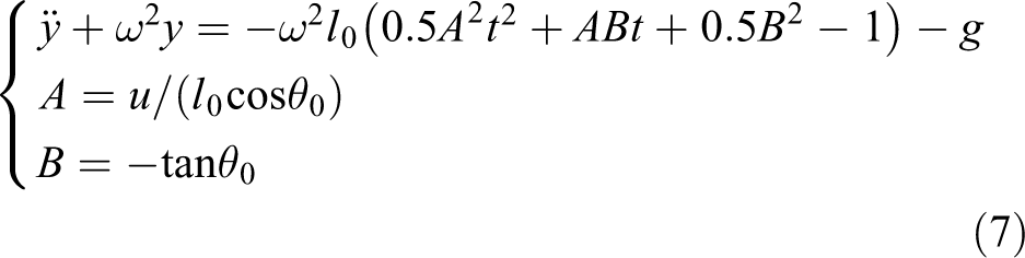
\{\begin{matrix} \ddot{y} + ω^{2} y = - ω^{2} l_{0} (0.5 A^{2} t^{2} + A B t + 0.5 B^{2} - 1) - g \\ A = u / (l_{0} cos θ_{0}) \\ B = - tan θ_{0} \end{matrix}

The general solution of equation (7) consists of a linear combination of the solution from the homogeneous differential equation and a special solution from the inhomogeneous equation generated by the undetermined coefficient method as equation (8)

y (t) = C_{1} cos (ω t) + C_{2} sin (ω t) + a t^{2} + b t +c

Also, the first-order derivative of equation (8) is

\dot{y} (t) = - C_{1} ω sin (ω t) + C_{2} ω cos (ω t) + 2 a t + b

By combining the three equations above and substituting the initial boundary conditions below (equation (10)), we obtain the coefficients of the general solution in equation (11)

\{\begin{matrix} y (t = 0) = l_{0} c o s θ_{0} \\ \dot{y} (t = 0) = v_{y 0} \end{matrix}

\{\begin{cases} C_{1} = (0.5 B^{2} + cos θ_{0} - 1) l_{0} + (g - A^{2} l_{0}) / ω^{2} \\ C_{2} = (v_{y 0} + A B l_{0}) / ω \\ a = - 0.5 A^{2} l_{0} \\ b = - A B l_{0} \\ c = l_{0} - 0.5 B^{2} l_{0} + (A^{2} l_{0} - g) / ω^{2} \end{cases}

The symmetry assumption (b) helps to reduce the dimension of ω that the spring is deflected to its maximum and the vertical velocity of the COM is zero at mid-stance

\dot{y} (t = T_{s 0} / 2) = 0

Substitute equation (12) into equation (9), we get the symmetric function

C_{1} ω sin (ω T_{s0} / 2) - C_{2} ω cos (ω T_{s0} / 2) = a T_{s0} + b

To solve ω, we introduced a new angular variable ϕ and scalar r. They satisfy the following definitions

\{\begin{cases} r = ω \sqrt{C_{1}^{2} + C_{2}^{2}} \\ sin φ = C_{2} ω / r \\ cos φ = C_{1} ω / r \end{cases}

equation (13) can be rewritten as followed

r [sin (ω T_{s 0} / 2) cos φ - cos (ω T_{s 0} / 2) sin φ] = a T_{s 0} + b

thus

sin (ω T_{s 0} / 2 - φ) = (a T_{s} + b) / r

With the equation (3), we were surprised to find that

a T_{s 0} + b = \frac{u (2 l_{0} sin θ_{0} - u T_{s})}{2 l_{0} {cos}^{2} θ_{0}} =0

which means that

\{\begin{cases} φ = ω T_{s 0} / 2 \\ tan φ = C_{2} / C_{1} \end{cases}

Unfortunately, C ₁, C ₂ are polynomial coefficients containing ω. We need to use Taylor expansion to solve the function since equation (18) is an implicit form. As we all know from traditional stance time estimation that T _s0 ≈ T/2, thus ωT _s0/2 ≈ π/2, which means that a duplication formula has to be used to achieve acceptable accuracy of Taylor expansion. As a trade-off, we used the triple-angle-formula

tan (\frac{ω T_{s 0}}{2}) = \frac{3 tan (ω T_{s 0} / 6) - {tan}^{3} (ω T_{s 0} / 6)}{1 - 3 {tan}^{2} (ω T_{s 0} / 6)} \approx \frac{108 T_{s 0} ω - ω^{3} T_{s 0}^{3}}{216 - 18 T_{s 0}^{2} ω^{2}}

For the convenience of reading, we stipulate that

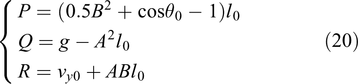
\{\begin{cases} P = (0.5 B^{2} + cos θ_{0} - 1) l_{0} \\ Q = g - A^{2} l_{0} \\ R = v_{y 0} + A B l_{0} \end{cases}

thus

\frac{108 T_{s 0} ω - ω^{3} T_{s 0}^{3}}{216 - 18 T_{s 0}^{2} ω^{2}} = \frac{C_{2}}{C_{1}} \frac{R ω}{P ω^{2} + Q}

Since ω ² = K _leg/m, the function can be simplified as

T_{s 0}^{3} P {(ω^{2})}^{2} + (Q T_{s 0}^{3} - 18 R T_{s 0}^{2} - 108 P T_{s 0}) (ω^{2}) + (216 R - 108 T_{s 0} Q) = 0 (θ_{0} > 0)

With the computerized assistance we obtained the symbols of the coefficients in this quadratic equation and the solution

\{\begin{cases} Δ = {(Q T_{s 0}^{3} - 18 R T_{s 0}^{3} - 108 P T_{s 0})}^{2} - 4 T_{s 0}^{3} P (216 R - 108 T_{s 0} Q) \\ K_{leg} = m ω^{2} = [\sqrt{Δ} - (Q T_{s 0}^{3} - 18 R T_{s 0}^{2} - 108 P T_{s 0})] / (2 T_{s 0}^{3} P) \end{cases}

So far, equation (23) constitutes the approximate analytical description of the leg stiffness of a high-speed system in passive motion. An accurate and stable stiffness could be obtained by one-step calculation compared with the multistep integrations and iterations in the numerical method.

It is important to note that, with the symmetric character, although the formula is derived on the scenario that the leg swings to its maximum touch angle θ ₀ in high-speed running, the approximation can also be applied to low-speed running while θ _td < θ ₀ based on the following definition

\{\begin{cases} T_{s 0} = T_{s_specify} \\ θ_{0} = arc sin (u T_{s_specif y} / (2 l_{0})) \end{cases}

where T _{s_specify} is the stance time specified by the programmer.

Stiffness strategy

High-speed running animals have their own stiffness strategy. Step-length adjustment is the first choice of speed regulation in the low-speed movement. However, due to the limitation of structure and friction cone, further speed improvement can only be achieved by increasing leg stiffness and reducing the stance time.³⁰ Based on the biological characteristics, a pre-calculated touchdown angle (θ _{0_pre}) deduced by the desired speed and the target stance time will be treated as the basis for strategy switching. As depicted in Figure 2.

Figure 2.

Process of stiffness selection in analytical solution.

When θ _{0_pre} < θ ₀, the touchdown angle increases with speed, while the stance time remains constant. θ _td = θ _{0_pre}.

When θ _{0_pre} ≥ θ ₀, the stance time decreases with speed, while the touchdown angle retains as θ ₀·θ _td = θ ₀.

Numerical simulation

We apply a numerical method in Matlab to evaluate the performance of the analytical solutions because the numerical method can obtain a sufficiently accurate solution satisfying locomotion details. The iterative process is shown in Figure 3.

Figure 3.

The monotonicity character and Newton method: (a) The monotonicity relationship between leg stiffness and stance time on the premise of a single variable (data from the simulation results in the next section) and (b) convergence function constructed by the Newton iteration method.

With the monotonicity^24
–26 of the function (see Figure 3(a)), we obtain a stance time with reasonable initial stiffness and state-values by Runge–Kutta method in the inner layer of the program and then construct an iteration formula in the outer layer to search the appropriate leg stiffness by the Newton-Iteration-method. The simulations are performed using the Runge–Kutta integrator, ode45 with event detection of leg touchdown and liftoff.

The analytical solutions of local linearization are used as the initial value of the search to accelerate the convergence speed since the Newton-iteration-method is sensitive to the initial values. The initial parameters of the SLIP model are set as in Table 1, which is close to the parameters of an adult cheetah.³⁵

Table 1.

Model parameters for iteration.

Nomenclature	Symbol	Value
Total mass	m	30 kg
Initial height of the COM	h ₀	0.8 m
Length of the leg	l ₀	0.65 m
Original stance time	T _s0	0.2 s
Maximum touchdown angle	θ ₀	25°

COM: center of mass.

In regard to the parameters, we systematically change the input parameters relevant to the locomotion. It is important to note that, similar to animals, the maximum touchdown angle at low speed was restricted to 15° and increased gradually to 30° below 3 m/s and keeps this final maximum touchdown angle even in higher speed. Thus, preventing the calculated leg from being too soft.

Co-simulation platform

The Adams-Matlab co-simulation platform was also used to simulate the real physical environment of single leg hopping as well as to test the control performances. Comparisons are taken between the effects of TMM and HMM method on the accuracy of stiffness estimation and stable performance.

As seen in Figure 4, the robot consists of three parts: the body, the thigh, and the shank. A rotational joint connects the thigh to the body and a translational joint connects the shank to the thigh. It is constrained to move along a straight planar path. A body mass of 30 kg has been chosen. This is approximately half of the mass of an adult cheetah, allowing us to compare to this cursorial runner. The mass ratio between the body and the leg is set to 20:1 to avoid a significant influence on body posture when leg swings and the mass of the leg is evenly distributed. The static and dynamic friction coefficients were set to 0.8/0.75 because the maximum touchdown angles of most cursorial animals are around 28.¹⁵

Figure 4.

The screenshot of co-simulation platform: Capture of the posture changes in one hopping cycle.

We adopted the well-regarded control strategy ‘Three-part Controller’ to manipulate rebound height, running speed and body attitude independently.³⁶ The forward speed was controlled by the ‘neutral point’ theory with speed sampling at the beginning of the flight phase and the actual stance time of the final hopping cycle was selected during the calculation of the touchdown angle.

Within the boundaries of the stiffness estimation model, the desired touchdown angle and the desired stance time also include the PID value of velocity deviation during the calculation process because feedback was applied in the actual control framework and the estimation model should use data that is consistent with reality.

Since actual locomotion systems must have energy dissipation and injection,³⁷ a damping ratio of 10 N·m/s was added to the translational joint to prevent leg tremor, also a rotational damping ratio of 10⁻⁶N·m·s/deg was added to the hip. A thrust was applied in the radius direction when the leg rebounds from the ground and the pitch angle was adjusted during the stance phase with a small hip torque.

The total hopping parameters used in the simulation are presented in Table 2.

Table 2.

Parameters in high-speed hopping.

Parameters	Value
Body mass	30 kg
Mass ratio between body and leg	20:1
Static friction coefficients	0.8
Dynamic friction coefficients	0.75
Maximum touchdown angle	25°
Translational damping ratio	10 N·m/s
Rotational damping ratio	5 × 10⁻⁷ N·m·s/deg
Acceleration	0.2 m/s² /0.1 m/s²
Initial stance time	0.2 s
Minimum stance time	0.07 s

To avoid the influence of acceleration on observation, we set up the acceleration process with a multistep approach with a time interval for each speed. The predetermined initial stance time is 0.2 s, and the minimum stance time in super high-speed is set to 70 ms because the leg inertia is insurmountable.

Result

Numerical simulation result

Comparisons between the analytical and numerical methods for the required leg stiffness are illustrated in Figure 5. As in Figure 5(a), the TMM method (red solid line) fits well with the numerical result (blue solid line) because the touchdown angle and velocity have been taken into account within the model. The maximum stiffness error is less than 12% even in ultra-high-speed, while the method of HMM draws a significant gap as the speed increased to 10 m/s, almost twice as much as other methods. The vertical stiffness ‘K _vert’ (Pink dotted line) which is derived from the leg stiffness of numerical results is highly consistent with Thomas’s findings¹⁵ when contrasting with K _leg.

Figure 5.

Stiffness increase with vertical speed: (a) Stiffness estimation results influenced by forwarding speed; (b) local enlargement of Figure 1(a); (c) stiffness estimation results influenced by the touchdown angle; and (d) stiffness estimation results influenced by the vertical velocity of the COM. COM: center of mass.

As seen in Figure 5(b), all these methods obtain a very similar stiffness prediction when forward velocity is less than 3 m/s. The HMM method is smaller than the numerical result at first and then grows significantly at the high-speed component, while the TMM method remains a little larger than the numerical result. Due to the limitation of Taylor’s expansion accuracy (Higher accuracy requires solving the complex quaternary equation), the TMM method could not fit with the numerical result completely. On the other hand, the symmetry of the numerical simulation is influenced by the assumption of constant forward velocity, which may cause the deviation of the touchdown angle from the theoretical value. It can also be seen in Figure 5(b) that leg stiffness increases dramatically with maximum touchdown angle θ ₀ becomes steeper since a smaller step length requires a much shorter stance time.

In Figure 5(c), K _leg is plotted vs the vertical velocity v_y ₀, and it is apparent that K _leg increases approximately linearly with v_y ₀ as the forward velocity is set up as a constant value of 10 m/s.

By using different model results as the initial values of the numerical searching, the iteration time is presented in Figure 6(a). The TMM result is sufficiently close to the real value that most iterations can be completed within three steps, while HMM fits best at the intersection point but performs poorly in other points. As depicted in Figure 6(b), the stance time errors by substituting K _leg from TMM and HMM results also reveal the accuracy of the estimation, and the relative error trend in TMM is much smaller than HMM.

Figure 6.

The accuracy of the new analytical solution: (a) Iteration times by different initial values; the TMM method is sufficiently close to the real value that most iterations can be completed in three steps; (b) Error of stance time by different calculation method, the relative error in TMM is smaller than HMM. TMM: triangle motion model; HMM: harmonic motion model.

Adams-Matlab co-simulation

Despite the simplicity of the control law mentioned above, the simulation results show the stability of the forward speed, maximum height, and posture in both applications. However, detailed graphs in Figure 7 show a better velocity tracking with less fluctuation and higher stable speed by using the TMM method. Since the fluctuation in the stance time has a strong correlation with planned touchdown angle, the feedback system has to work consistently to compensate for the velocity changes during stance phase if the HMM method is adopted. The fluctuation is small in relation to velocity itself in high-speed locomotion, which is consistent with the assumptions of uniform horizontal velocity at stance phase.

Figure 7.

Velocity tracking: (a) velocity tracking by TMM method. The TMM method achieves a higher and more stable speed without oscillation; (b) velocity tracking by HMM method. TMM: triangle motion model; HMM: harmonic motion model.

Figure 8 (a) and (b) shows the leg sweep angle and its symmetricity during stance by TMM method. The magnitude of asymmetry during stance is relatively small when compared with the touchdown angle, which clarifies the validity of assumption (b). Due to the feedback within the physical system, the desired stance time in Figure 8(c) and (d) varied slightly with different methods. But the stance time in the TMM method is fundamentally consistent with the desired stance time, particularly during the high-speed interval (3–8 m/s). Yet the HMM method has considerable deviations at low-speed and high-speed sections and the minimum deviation occurs around 3 m/s, which is the intersection point of the two stiffness curves in Figure 6(b). What can be found particularly is the highly consistency of the stance time errors between Figure 6(b) and Figure 8. These phenomena were caused by the fact that HMM adopts lower stiffness at low speed, while much higher stiffness at high speed. Compared with the ultra-short stance time in ultra-high-speed locomotion, any small error will have an impressive effect on stability.

Figure 8.

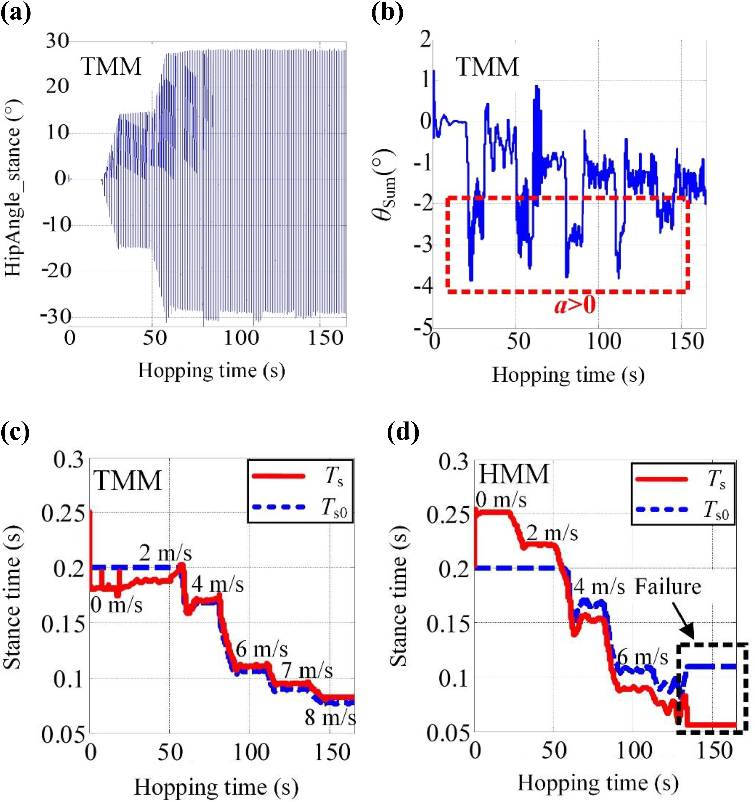
Hip angle performance and stance time comparison: (a) Leg sweep angle in stance time by TMM method; (b) the representative $P_{a s y m} = θ_{t d} + θ_{l o}$ to show the magnitude of symmetricity; (c) stance time obtained by TMM and HMM method; and (d) stance time obtained by the HMM method. TMM: triangle motion model; HMM: harmonic motion model.

The stiffness applied in the simulation and the corresponding effects on leg swing angles during the stance phase were presented in Figure 9. Due to the feedback loop, the control system can adjust the touchdown angle in real time to ensure the symmetry as long as possible. Although some disturbance exists in the actual physical system of TMM method such as the ground impact and motion delay caused by the inertia (Figure 9 (b)), the sweep angle in the TMM method is fully utilized and has a more stable performance than HMM. The HMM method generated a much narrow and unstable leg sweep angle in high speed owing to the great increment in leg stiffness.

Figure 9.

The stiffness adopted and the corresponding effect: (a) The HMM method adopts a much higher stiffness in high-speed section and (b) the sweep angles during stance by TMM and HMM show that the sweep angle in the TMM method is fully utilized. TMM: triangle motion model; HMM: harmonic motion model.

Discussion

A vital question regarding the stiffness selection in high-speed locomotion is how to limit maximum stiffness? The solution of leg stiffness in the TMM method mimics a similar result as speed increased to more than 10 m/s, even though it is not shown here because ultra-high-speed locomotion with a single leg is still quite difficult for a real robot limited by leg inertia, structural strength, and actuators.

Based on the consistent ground impulse received in a steady-state, the average GRF acting on the toe will increase significantly with the shortening of stance time. Although some methods can be taken to alleviate the ground impact, such as leg retraction before landing, the increase of impact force is inevitable and excessive impact may cause the fracture of mechanical structures. High stiffness also requires the actuators to generate a high force at a high frequency in active stiffness since the damper diminish significantly more mechanical energy as the impact force is increased. A mass–spring–damper (MSD) model developed by Alexander et al.³⁸ also helps to highlight the relationship between leg stiffness and paw-pad stiffness in that it should not exceed five times of paw-pad stiffness in order to prevent chatting on the toe. These limitations make it impossible for us to increase leg stiffness infinitely.

Alternatively, if the compliance is too soft, it cannot provide a sufficient buffering force within the allowable compression range to balance the weight and resist the landing shock by squeezing energy into the spring. A softer leg may also degrade the positioning accuracy of the foot, and bigger amplitude of torso vibration caused by the compliance would add more noise and decrease sensing accuracy of the sensors on the back.

The TMM method for calculating leg stiffness is helpful to get real-time stiffness quickly through these complex boundaries in high-speed running. The accurate solution also helps to reduce the risk of using a much stiffer leg or much softer leg to harm the structure.

The Multi-leg cooperation with different gaits or spine movement could play a much more significant role in achieving a higher speed mission after the Limited Stance Time (LST) appeared.

Conclusions

Leg stiffness plays an essential role in touchdown angle and speed regulation. In relation to the HMM model, we propose a TMM model to solve the approximate analytical solution of stiffness in high-speed running. The TMM method accurately grasps the characteristics of high-speed running in that large range of leg sweep angle and small fluctuation of the COM occur. Both the numerical simulation and the multi-body dynamics simulation in ADAMS show the accuracy of the TMM method in the accurate prediction of leg stiffness even in ultra-high-speed. It is also adaptable to low speed and small sweep angle cases. The accurate solution of this model also helps the structure of the robots to avoid damage caused by a much stiffer leg or a much softer leg. Its accurate solution has a great advantage on velocity tracking and leg sweep angle utilizing as well as the system stability.

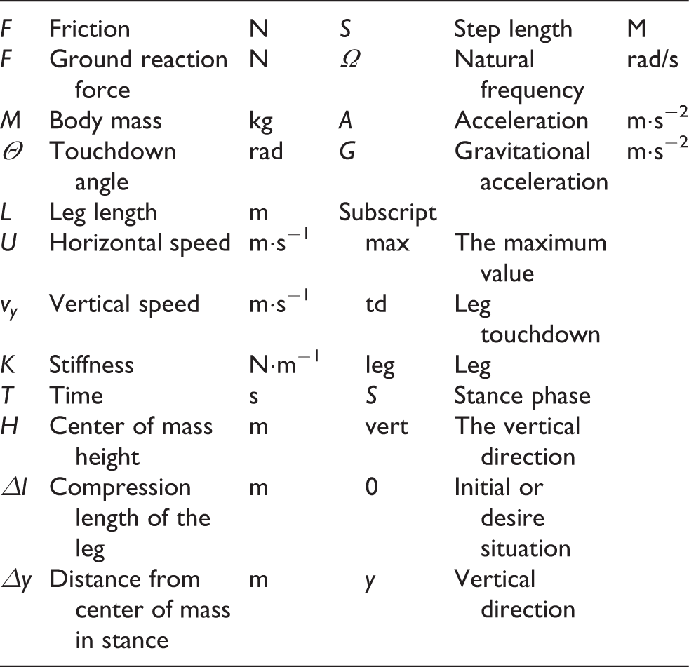
Nomenclatures

F	Friction	N	S	Step length	M
F	Ground reaction force	N	Ω	Natural frequency	rad/s
M	Body mass	kg	A	Acceleration	m·s⁻ ²
Θ	Touchdown angle	rad	G	Gravitational acceleration	m·s⁻ ²
L	Leg length	m	Subscript
U	Horizontal speed	m·s⁻¹	max	The maximum value
v_y	Vertical speed	m·s⁻ ¹	td	Leg touchdown
K	Stiffness	N·m⁻ ¹	leg	Leg
T	Time	s	S	Stance phase
H	Center of mass height	m	vert	The vertical direction
Δl	Compression length of the leg	m	0	Initial or desire situation
Δy	Distance from center of mass in stance	m	y	Vertical direction

Footnotes

Declaration of conflicting interests

The author(s) declared no potential conflicts of interest with respect to the research, authorship, and/or publication of this article.

Funding

The author(s) disclosed receipt of the following financial support for the research, authorship, and/or publication of this article: This work was supported by Natural Science Foundation of China (No.61773139 and No.U1713222), Shenzhen special fund for future industrial development (No.JCYJ20160425150757025) and Shenzhen Peacock Plan (No.KQTD2016112515134654).

ORCID iD

Changrong Cai

References

Park

Kim

. Quadrupedal galloping control for a wide range of speed via vertical impulse scaling. Bioinspir Biomim 2015; 10: 025003.

Seok

Wang

Michael Chuah

, et al. Design principles for energy-efficient legged locomotion and implementation on the MIT Cheetah Robot. IEEE/ASME Trans Mech 2015; 20: 1117–1129.

Huang

Zhang

, et al. High-order disturbance observer based sliding mode control for mobile wheeled inverted pendulum systems. IEEE Transactions on Industrial Electronics 2019; 1–1.

Chen

Carbonari

Canali

, et al. Design of a novel dexterous robotic gripper for in-hand twisting and positioning within assembly automation. Assembly Autom 2015; 35: 259–268.

Raibert

Blankespoor

Nelson

, et al. Bigdog, the rough-terrain quadruped robot. IFAC Proc Vol 2008; 41: 10822–10825.

Muybridge

Brown

. Animals in motion. Courier Corporation 2012; 25–63.

Blickhan

. The spring-mass model for running and hopping. J Biomech 1989; 22: 1217–1227.

Alexander

. Three uses for springs in legged locomotion. Int J Rob Res 2016; 9: 53–61.

Raibert

Tello

. Legged robots that balance. Cambridge, MA: MIT press, 1986, pp. 89–89.

10.

Kim

Clark

Cutkosky

. iSprawl: design and tuning for high-speed autonomous open-loop running. Int J Robot Res 2006; 25: 903–912.

11.

Lee

Dong

Ahn

, et al. On the dynamics of a quadruped robot model with impedance control: self-stabilizing high speed trot-running and period-doubling bifurcations. In: IEEE/RSJ international conference on intelligent robots & systems, Chicago, IL, USA, 14–18 September 2014. USA: IEEE.

12.

Greenemeier

. Running robots: see Boston Dynamics’s Speedy Cheetah in Action [Video]. 9 July 2012.

13.

Lewis

Bunting

Salemi

, et al. Toward ultra high speed locomotors: design and test of a cheetah robot hind limb. In: IEEE international conference on robotics & automation 2011, Shanghai, China, 9–13 May 2011, China: IEEE.

14.

Wang

, et al. Bio-inspired controller for a robot cheetah with a neural mechanism controlling leg muscles. J Bionic Eng 2012; 9: 282–293.

15.

Farley

Glasheen

McMahon

. Running springs: speed and animal size. J Exp Biol 1993; 185: 71–86.

16.

Ferris

Louie

Farley

. Running in the real world: adjusting leg stiffness for different surfaces. Proc Biol Sci 1998; 265: 989–994.

17.

Kerdok

Biewener

McMahon

, et al. Energetics and mechanics of human running on surfaces of different stiffnesses. J Appl Physiol (1985) 2002; 92: 469–478.

18.

Jiang

Wang

, et al. Control of a quadruped robot with bionic springy legs in trotting gait. J Bionic Eng 2014; 11: 188–198.

19.

Semini

Barasuol

Boaventura

, et al. Is active impedance the key to a breakthrough for legged robots? In: Robotics Research. Cham: Springer, 2016, pp. 3–19.

20.

Kram

McMahon

. Mechanics of running under simulated low gravity. J Appl Physiol (1985) 1991; 71: 863–870.

21.

Kram

Taylor

. Energetics of running: a new perspective. Nature 1990; 346: 265–267.

22.

Luhtanen

Komi

. Force-, power-, and elasticity-velocity relationships in walking, running, and jumping. Eur J Appl Physiol Occup Physiol 1980; 44: 279–289.

23.

Mero

Komi

PV.

Force-, EMG-, and elasticity-velocity relationships at submaximal, maximal and supramaximal running speeds in sprinters. Eur J Appl Physiol Occupat Physiol 1986; 55: 553–561.

24.

Farley

Gonzalez

. Leg stiffness and stride frequency in human running. J Biomech 1996; 29: 181–186.

25.

McMahon

Cheng

GC.

The mechanics of running: How does stiffness couple with speed?

J Biomech 1990; 23: 65–78.

26.

Kim

Park

. Leg stiffness increases with speed to modulate gait frequency and propulsion energy. J Biomech 2011; 44: 1253–1258.

27.

Herr

McMahon

. A trotting horse model. Int J Rob Res 2016; 19: 566–581.

28.

Arampatzis

Bruggemann

Metzler

. The effect of speed on leg stiffness and joint kinetics in human running. J Biomech 1999; 32: 1349–1353.

29.

Witte

Knill

Wilson

. Determination of peak vertical ground reaction force from duty factor in the horse (Equus caballus). J Exp Biol 2004; 207: 3639–3648.

30.

Zha

Wang

Wei

, et al. Research on the control method for high speed locomotion legged robot. In: International conference on advanced robotics & mechatronics 2018. Singapore City, Singapore, 18–20 July 2018. Singapore: IEEE.

31.

Ahmadi

Buehler

. Stable control of a simulated one-legged running robot with hip and leg compliance. IEEE Trans Robot Automat 1997; 13: 96–104.

32.

Thompson

Raiber

. Passive dynamic running. In: International Symposium on experimental robotics I, Montréal, Canada, 19–21 June 1989.

33.

Geyer

Seyfarth

Blickhan

. Spring-mass running: simple approximate solution and application to gait stability. J Theor Biol 2005; 232: 315–328.

34.

Cai

. Approximating the stance map of the SLIP runner based on perturbation approach. In: IEEE international conference on robotics & automation 2012, Saint Paul, MN, USA, 14–18 May 2012, pp. 4197–4203. USA: IEEE.

35.

Hudson

Corr

Wilson

. High speed galloping in the cheetah (Acinonyx jubatus) and the racing greyhound (Canis familiaris): spatio-temporal and kinetic characteristics. J Exp Biol 2012; 215: 2425–2434.

36.

Guo

Cai

, et al. A parallel actuated pantograph leg for high-speed locomotion. J Bionic Eng 2017; 14: 202–217.

37.

Ahn

Hogan

. A simple state-determined model reproduces entrainment and phase-locking of human walking. Plos One 2012; 7: e47963.

38.

Alexander

Bennett

Ker

. Mechanical properties and function of the paw pads of some mammals. J Zool 1986; 209: 405–419.

Estimation of leg stiffness using an approximation to the planar spring–mass system in high-speed running

Abstract

Keywords

Introduction

Problem formulation

Method

Approximating the stance phase

Stiffness strategy

Numerical simulation

Co-simulation platform

Result

Numerical simulation result

Adams-Matlab co-simulation

Discussion

Conclusions

Nomenclatures

Footnotes

Declaration of conflicting interests

Funding

ORCID iD

References