Robust improvement solution to perspective-n-point problem

Abstract

Perspective-n-point is a classical computer vision problem that uses three-dimensional points and image pixels to estimate camera pose. The visual robot often loses its position when the camera moves too fast or the environment changes. Perspective-n-point is used to relocate robot position, but the distribution of three-dimensional points in the world frame and different choices of coordinates affect the perspective-n-point performance and make perspective-n-point results less robust and inaccurate. In this study, we review the previous perspective-n-point algorithms and provide their disadvantages when facing three-dimensional points with large variances. According to the drawbacks of previous perspective-n-point methods, we propose a normalization method inspired by the homogeneous matrix calculation process to increase perspective-n-point algorithm accuracy and robustness. The experimental results demonstrate that the proposed perspective-n-point method is robust to different choices of coordinates and is thus better than other state-of-art perspective-n-point methods. Considering that the true camera pose is difficult to obtain, the former perspective-n-point solution validation experiment is mostly based on simulated image data. In this study, we design a new experiment based on total station and chessboard to verify the robustness and accuracy of the perspective-n-point algorithm.

Introduction

There are three main geometry problems in multiple computer vision: the homography problem, ^1,2 iterative closest point (ICP) problem, ^3,4 and perspective-n-point (PnP) problem. ^{5 –8} The PnP problem focuses on reconstructing camera absolute pose using known image pixels and three-dimensional (3-D) points in world space, which is a widely studied problem in computer vision, ⁹ such as in augmented reality, ¹⁰ simultaneous localization and mapping (SLAM) pose recovery in loss of frames, ¹¹ and vision localization in smart cities.

For example, effects of dynamic environments, illumination change, and occlusion of sight are unavoidable in visual navigation and localization. Thus, a PnP algorithm is used to relocate the robot position when a robot loses its positions. According to common intuition, different selections of known 3-D points does not affect PnP algorithm results very much, and the absolute pose in the world should be close to the true value. However, our experiments demonstrate that this intuition is false. If the x-, y-, and z-axes of 3-D points do not distribute equally in the world frame, the final absolute pose in the world frame will change significantly with different selections of 3-D points and be far away from the true pose. Experiments are shown in the “Results” section, which demonstrate that previous PnP algorithms cannot perform very well if 3-D points are distributed unequally.

First, considering the inaccurate and unstable performance of previous PnP methods under the unequally distributed 3-D points scenario, we propose a normalization method using a principal component analysis (PCA) technology, which makes PnP results more stable. The idea is inspired by the homography matrix calculation. ¹ The normalization process aims to average the cost function matrix and singular-value-decomposition (SVD) matrix so that the magnitude of every element is close to each other, which makes condition numbers as small as possible. ¹² At the same time, we abandon the traditional pose transformation model Rp + t considering the defect of the PnP algorithm, which enlarges the rotation matrix error. In this article, we choose the R (p − c) pose transformation model, which is more robust than the traditional pose transformation model.

Second, we design a new experiment using total station, an electronic/optical instrument used for surveying, building construction, and 3-D chessboards, to evaluate previous PnP methods. Before executing the robust test program, two key points must be confirmed. The first is the position variance of 3-D points. In earlier works, ^{13 –20} only simulated data were used, which generates world frame 3-D points in the regions [1, 2] × [1, 2] × [4, 8] or [1, 2] × [−2, 2] × [4, 8]. In our experiment, we use GPS-RTK to obtain GPS coordinates of total station and then use total station to obtain chessboard coordinates. x-, y- and z-ranges are [−1845992, −1845991] × [870837, 870838] × [−2928936, −2928935]. To prevent planar PnP from happening and to help extract feature points in images, we place three chessboards on the three faces of the trihedron as shown in Figure 1. The second point to confirm is true camera pose. True camera pose in the world frame is obtained by the average of 3-D points in the camera frame. In our experiment, we use intrinsic parameters from a MYNT-EYE stereo camera. Experimental results presented in the “Results” section show that our proposed method is better than the state-of-art PnP algorithm, especially in terms of robustness in a real scene. The previous PnP algorithms show high accuracy using simulated data, but the performance is very poor in our designed experiment. The main reason is that the former PnP experimental 3-D points in improving the world only exist in the region [1, 2] × [1, 2] × [4, 8] or [1, 2] × [−2, 2] × [4, 8], and the spatial differentiation between these 3-D points is very small.

Figure 1.

Trihedron constructed using three chessboards.

The rest of this study is organized as follows: In the “Related work” section, we review state-of-art PnP algorithms and analyze their drawbacks. In the “Normalization of PnP method” section, we describe the details of the proposed PnP algorithm and analyze the reason it performs better than state-of-art PnP methods. In the “Results” section, experiments using simulated data are shown, and our newly designed experiment introduced. Finally, we compare several kinds of PnP algorithms, including the proposed one, using real-world scenarios.

Related work

In recent years, PnP algorithms have been widely studied in the domains of robotics and computer vision. They myriad kinds of methods are different from each other but can be divided into two main kinds: optimization solutions and analytical solutions. An optimization solution forms an effective cost function with which to describe PnP camera projection, and a Gauss–Newton or Levenberg–Marquardt optimal algorithm is used to obtain expected results iteratively. The optimization method’s drawback is that it relies too much on the initial camera pose value. Nonlinear optimization cannot obtain all of the stationary points and cannot guarantee that the final convergence solution is the true solution because different initial poses converge to their nearest stationary point instead of the true camera pose. An analytical solution is sensitive to data noise and outliers, so it is often polished using the optimization method.

The DLT ²¹ PnP method is the naive analytical PnP method that transforms the PnP problem equation (1) directly into the linear homogeneous equation (2) problem

$s_i\left[\begin{array}{c}{u\prime }_i\\ {v\prime }_i\\ 1\end{array}\right]=\left[\begin{array}{cccc}{r}_{11}& r_{12}& r_{13}& t_x\\ r_{21}& r_{22}& r_{23}& t_y\\ r_{31}& r_{32}& r_{33}& t_z\end{array}\right]\left[\begin{array}{c}x\\ y\\ z\\ 1\end{array}\right]$

1

$\left[\begin{array}{cccccccccccc}x& y& z& 1& 0& 0& 0& 0& -{u\prime }_{i}x& -{u\prime }_{i}y& -{u\prime }_{i}z& -{u\prime }_i\\ 0& 0& 0& 0& x& y& z& 1& -{v\prime }_{i}x& -{v\prime }_{i}y& -{v\prime }_{i}z& -{v\prime }_i\end{array}\right]\left[\begin{array}{c}{r}_{11}\\ r_{12}\\ r_{13}\\ t_x\\ r_{21}\\ r_{22}\\ r_{23}\\ t_y\\ r_{31}\\ r_{32}\\ r_{33}\\ t_z\end{array}\right]=0$

2

[x, y, z, 1]^T is the 3-D point coordinate in the world frame. ${\left[u_i^{\prime },v_i^{\prime },1\right]}^{\text{T}}$ is the image pixel that is the observation of 3-D point [x, y, z, 1]^T, and $\text{[}Rt\text{]}=\left[\begin{array}{cccc}{r}_{11}& r_{12}& r_{13}& t_x\\ r_{21}& r_{22}& r_{23}& t_y\\ r_{31}& r_{32}& r_{33}& t_z\end{array}\right]$ is the estimated camera pose matrix. We continue using these notations in this article. We can use SVD factorization to obtain equation (2), but we do not fully consider pose-matrix properties, such as rotation matrix’ orthogonality. Thus recovering the pose matrix from equation (2) produces large pose errors compared with other PnP methods.

The LHM ²² method is an optimization PnP method that first obtains the initial camera pose in the world frame using a weak-perspective model ¹ and then forms a cost function called an image-space collinearity equation to obtain the final convergent solution. The traditional iterative PnP cost function is based on image observation error, but the image-space collinearity cost function takes 3-D space position error into consideration, which increases spatial constraint robustness. The LHM method fully exploits the structure of the pose matrix and converts the PnP problem into the iterative ICP problem. Under the weak-perspective assumptions, we believe that all of 3-D points in the world frame are parallel to the image plane. This is the drawback of the LHM method, namely that all of the 3-D points conforming to the weak-perspective model in the real scene cannot be guaranteed. If the initial pose matrix is too far from the true solution, then the iterative direction may not advance to the global optimal solution.

According to the drawback of the LHM method mentioned above, Schweighofer and Pinz ²³ pointed out that the LHM image-space collinearity cost function is one of the reasons for pose ambiguities when all the 3-D points are coplanar. The LHM + SP algorithm is designed to solve this problem. In fact, the LHM + SP algorithm is just a variant of the optimization PnP method that only increases LHM robustness in the coplanar situation. Therefore, the LHM + SP algorithm also relies on the weak-perspective model which is also not satisfied in the real scene.

The most famous and most widely used noniterative PnP algorithm is EPnP, ¹³ which decreases computational cost and makes it possible for the method to run in real time. The central idea of the EPnP method is to transform the EPnP problem into ICP problem. If one can obtain 3-D points in the camera coordinates in a certain way, the remaining work can be finished using the ICP algorithm. The EPnP algorithm constructs a new coordinate obtained by conducting PCA analysis of input 3-D points in the world frame. Coordinate transformation does not change the distances between 3-D points and the EPnP utilizes this property to obtain the transformation between camera coordinates and new coordinates, so the 3-D points in the camera coordinates can be easily obtained. However, the last step of the EPnP algorithm is the alignment of 3-D points in the world coordinates and camera coordinates, and this step cannot guarantee that the 3-D points in the world coordinates have a positive z-axis value. A negative z-axis value means that the observed 3-D point is behind the camera, which does not obey physical laws.

The DLS method ¹⁴ was the first robust noniterative PnP method. The DLS method constructs a cost function that is very similar to the LHM cost function. Figure 2 describes the difference between the DLS and LHM cost functions. P is the 3-D point in the camera frame, which is obtained by P _camera = RP_world + t. P _world is the input 3-D point in the world frame. The direction of line L2 in the camera frame is determined by the normalized image pixel ${\left[u_i^{\text{'}},v_i^{\text{'}},1\right]}^{\text{T}}$ and the direction of line L3 in the camera frame is determined by P _camera. P1′ is the intersection of lines L2 and L1, which is perpendicular to L3 and intersects L2. P _camera − P1′ is the LHM defined error. A strong assumption is made that the 3-D point P1′ that is recovered by the normalized image point ${\left[u_i^{\text{'}},v_i^{\text{'}},1\right]}^{\text{T}}$ must be the intersection of lines L1 and L2. Obviously, the assumption does not conform to the real data noise situation. The DLS method adds a new estimated parameter with which to solve this problem perfectly. The new estimated parameter is the distance α between the camera center and 3-D point. Therefore, P2′ can be expressed as

$P2\prime =\frac{\alpha {[\begin{array}{ccc}{u}_i^{\prime }& v_i^{\prime }& 1\end{array}]}^{\text{T}}}{\Vert {[\begin{array}{ccc}{u}_i^{\prime }& v_i^{\prime }& 1\end{array}]}^{\text{T}}\Vert }$

3

Figure 2.

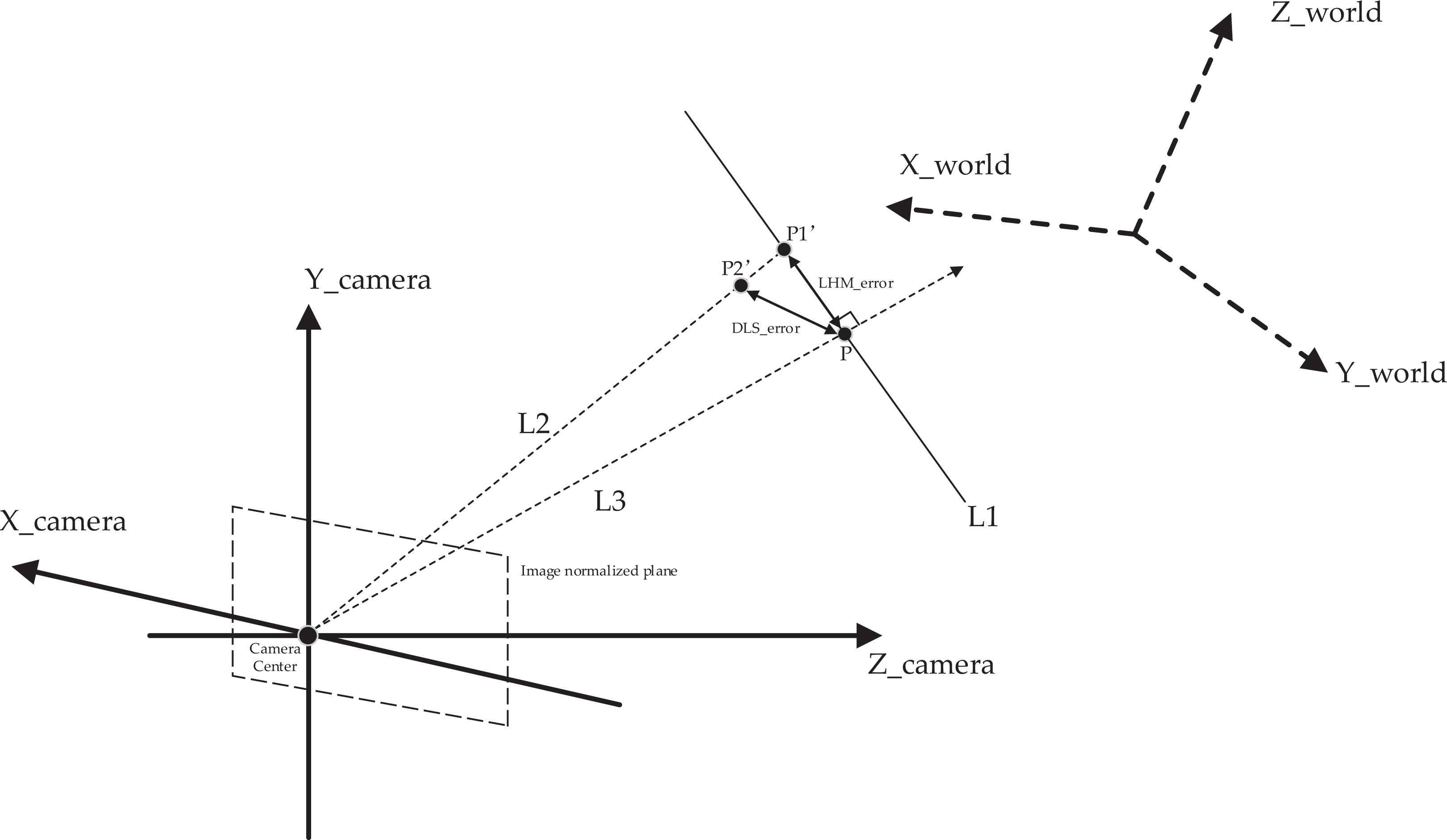
Differences between DLS and LHM methods. P is the 3-D point in the camera frame, P _world the input 3-D point in the world frame, and P _camera the 3-D point in the camera frame.

The DLS error is the distance between P2′ and P as depicted in Figure 2. The DLS method does not use an iterative optimization method to solve the cost function like the LHM method does. The DLS method introduces CGR parameters to represent the estimated rotation matrix R and converts the nonlinear cost function to the polynomial system problem without a weak-perspective model guess of an initial value. The Macaulay matrix is applied to solve all of the critical points of the polynomial equations. In all of the critical points, we obtain a single critical point as the solution of minimizing the cost function. Although the DLS method solution is robust and analytical, it does not perform well in cases of 180° rotations around the x-, y-, and z-axes because of the drawbacks of CGR parameterization.

The RPnP method ¹⁵ is based on the classical P3P ¹⁶ method that converts a P3P constraint equation to a fourth-order polynomial. The RPnP method does not employ linearization technology ¹⁷ to solve this polynomial but employs an eigenvalue method ¹⁸ to obtain the four minima of the polynomial. After solving the polynomial, 3-D points in the camera pose are obtained. The RPnP method does not use ICP directly to calculate camera pose. RPnP chooses to form a new coordinate frame to normalize 3-D points in the camera frame, which is similar to the proposed method, but RPnP also does not perform very well, like other PnP algorithms using large spatial differentiation of 3-D points. The main reason is that 3-D points in the camera frame are used upon normalization instead of the 3-D points in the world frame. The spatial differentiation of 3-D points in the camera frame is much smaller compared with 3-D points in the world frame, so the normalization process in the camera frame does not improve accuracy. RPnP method experimental results are compared with the proposed method and other PnP algorithms in the “Results” section.

The OPnP method ¹⁹ inherits the DLS core idea: form a cost function, parameterize rotation matrix R, and use a polynomial root method to obtain all of the stationary points of the cost function. Parameterization of R in the OPnP method uses a nonunit quaternion instead of the CGR parameter. A nonunit quaternion does not have any constraint, so the cost function is a nonconstrained optimization problem. ²⁰ Nonunit quaternion parameterization is not affected by the cases of 180° rotations around the x-, y-, and z-axes, so the OPnP algorithm is more robust than the DLS algorithm. However, the OPnP method is the same as the above-mentioned PnP methods, in that all of them do not consider the normalization process, which causes the PnP algorithm’s performance to be unstable. The comparisons between the above-mentioned PnP algorithms are shown in the Results section. We present their accuracy and robustness results in Figures 3 to 5 and Figures 6 to 13, respectively.

Figure 3.

Accuracy compared with EPnP, EPnP-GN, LHM, RPnP, DLS, OPnP, SP, and DLT algorithms without normalization process using simulated data. PnP: perspective-n-point.

Figure 4.

Magnified in RPnP, DLS, SP, and LHM results of Figure 11. PnP: perspective-n-point.

Figure 5.

Accuracy compared with EPnP, EPnP-GN, LHM, RPnP, DLS, OPnP, SP, and DLT with normalization process using simulated data. PnP: perspective-n-point.

Figure 6.

Rotation matrix fluctuation of PnP result in normalization frame. Right-hand-bottom figure presents angle-axis variance of eight PnP algorithms with normalization. PnP: perspective-n-point.

Figure 7.

Translation fluctuation of PnP result in normalization frame. Right-hand-bottom figure presents the translation variance of eight PnP algorithms with normalization. PnP: perspective-n-point.

Figure 8.

Rotation matrix fluctuation of PnP result in world frame using un-normalized data directly. Right-hand-bottom figure presents angle-axis variance of eight PnP algorithms without normalization. PnP: perspective-n-point.

Figure 9.

Translation fluctuation of the PnP result in world frame using un-normalized data directly. Right-hand-bottom figure presents translation variance of eight PnP algorithms without normalization. PnP: perspective-n-point.

Figure 10.

Location (c) fluctuation of PnP result in world frame using normalized data. Right-hand-bottom figure presents the location (c) variance of eight PnP algorithms with normalization. PnP: perspective-n-point.

Figure 11.

Translation (t) fluctuation of PnP result in world frame using normalized data. Right-hand-bottom figure presents the translation (t) variance of eight PnP algorithms with normalization. PnP: perspective-n-point.

Figure 12.

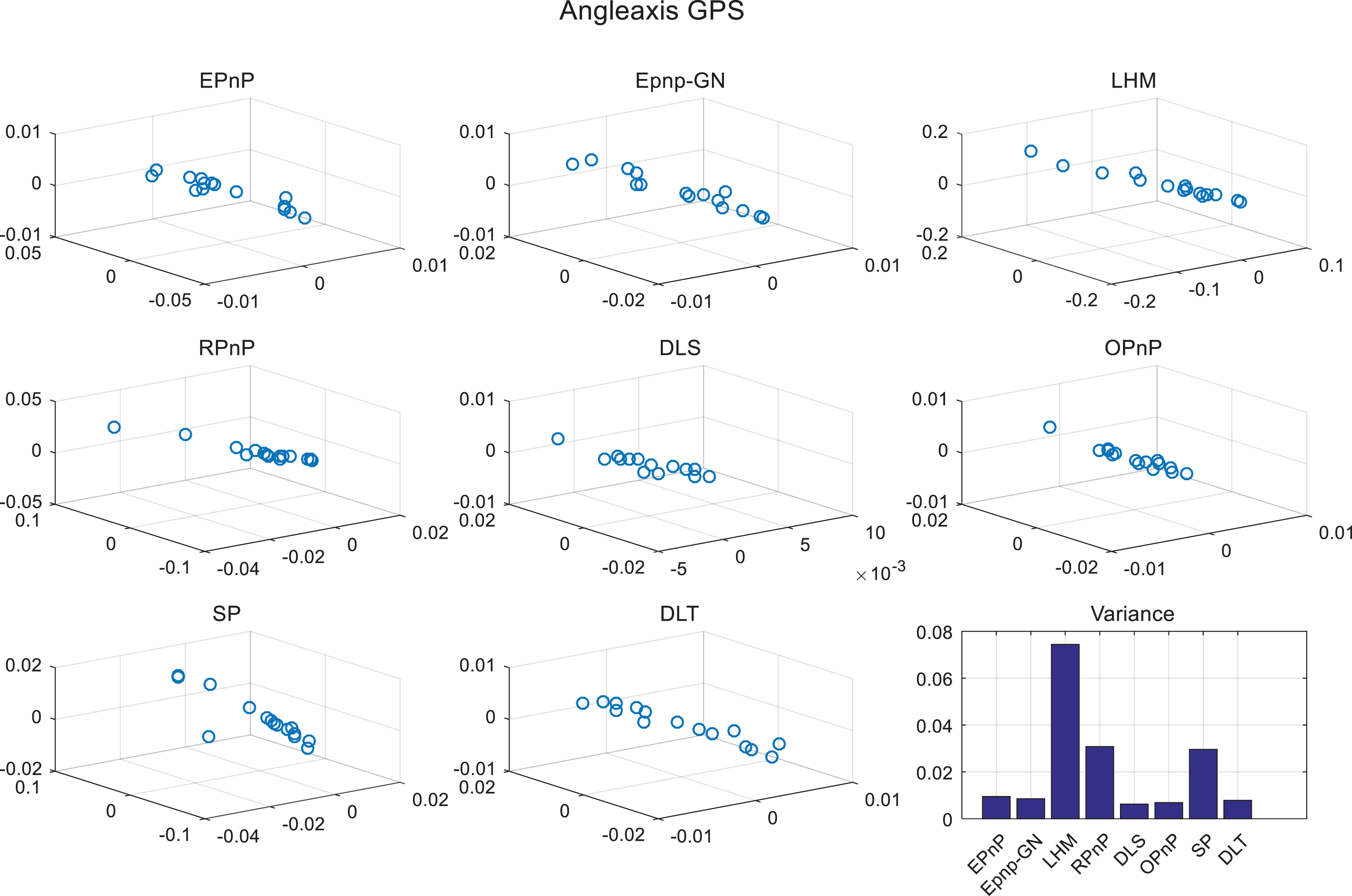
Rotation matrix fluctuation of the PnP result in world frame using normalized data. Right-hand-bottom figure presents the angle-axis variance of eight PnP algorithms with normalization. PnP: perspective-n-point.

Figure 13.

Points constrained error. The un-normalization results are yellow bars. The normalization results are blue bars.

Normalization of PnP method

Solving the linear homogeneous equation problem is often encountered in computer vision, such as in use of direct PnP algorithm in equation (2)

$Ax=0$

4

where A is equal to $\left[\begin{array}{cccccccccccc}x& y& z& 1& 0& 0& 0& 0& -{u\prime }_{i}x& -{u\prime }_{i}y& -{u\prime }_{i}z& -{u\prime }_i\\ 0& 0& 0& 0& x& y& z& 1& -{v\prime }_{i}x& -{v\prime }_{i}y& -{v\prime }_{i}z& -{v\prime }_i\end{array}\right]$ and x is equal to ${\left[\begin{array}{cccccccccccc}{r}_{11}& r_{12}& r_{13}& t_x& r_{21}& r_{22}& r_{23}& t_y& r_{31}& r_{32}& r_{33}& t_z\end{array}\right]}^{\text{T}}$ in equation (4). The column of A is n and the row of A is m. Rank(A) = n − 1 is the sufficient and necessary condition to guarantee the existence of a unique nonzero solution of (4). However, the input data A are often contaminated by noise, so the rank(A) = n. In this situation, SVD is often used to obtain the matrix A′ that is closest to A in the Frobenius norm and to ensure that rank(A′) = n − 1. Executing SVD of matrix A′: A′ = UD′V ^T. A = UDV ^T and D′ is D with the smallest singular value set to zero. It was proved in the study by Hartley ¹² that a smaller condition number of A ^T A produces a more stable SVD result, which means that the small changes of the matrix A will not lead to large changes of the SVD result. If the input 3-D point in the world frame is [10e4, 10e4, 10]. Equation (2) has a very large condition number because of the unbalanced value distribution in the matrix. One can see that the elements in the left-hand matrix with coefficients x and y are much larger than the elements with coefficient z. If we use SVD to calculate the solution of (2), the result will change significantly with different input points in the world frame. This occurs not only in the DLT method but also in the EPnP, LHM + SP, EPnP, DLS, RPnP, and OPnP algorithms. It is pointed out in Hartley and Zisserman ¹ and Hartley ¹² that the data normalization process can solve this problem.

We now introduce the normalization process into the PnP algorithm. We establish a new frame according to the input 3-D points in the world frame to guarantee that x _new, y _new, and z _new have the same order of magnitude. We call this new frame the normalized frame. [x _new, y _new, z _new]^T is the 3-D point in the normalized frame

$X=\left[\begin{array}{cccc}{x}_{1,\text{world}}-\overline{x_{\text{world}}}& x_{2,\text{world}}-\overline{x_{\text{world}}}& \mathrm{...}& x_{n,\text{world}}-\overline{x_{\text{world}}}\\ y_{1,\text{world}}-\overline{y_{\text{world}}}& y_{2,\text{world}}-\overline{y_{\text{world}}}& \mathrm{...}& y_{n,\text{world}}-\overline{y_{\text{world}}}\\ z_{1,\text{world}}-\overline{z_{\text{world}}}& z_{2,\text{world}}-\overline{z_{\text{world}}}& \mathrm{...}& z_{n,\text{world}}-\overline{z_{\text{world}}}\end{array}\right]$

5

where p_{i ,world} = [x_{i ,world} y_{i ,world} z_{i ,world}]^T, and $\overline{p_{\text{world}}}={\left[\begin{array}{ccc}\overline{x_{\text{world}}}& \overline{y_{\text{world}}}& \overline{z_{\text{world}}}\end{array}\right]}^{\text{T}}$ is the average point in the world frame. $R_{\text{convert}}X{X}^{\text{T}}{R}_{\text{convert}}{ }^{\text{T}}=Q$ . The PCA algorithm is used to find a transformation matrix $R_{\text{convert}}$ that can make Q a diagonal matrix. One can use SVD to obtain $R_{\text{convert}}: \text{SVD}(X{X}^{\text{T}})=UD{U}^{\text{T}}$ , and $R_{\text{convert}}=U^{\text{T}}$ and $t_{\text{convert}}=-R_{\text{convert}}\overline{p_{\text{world}}}$ are obtained by the PCA algorithm ²⁴

$R_{\text{convert}}{p}_{i,\text{world}}+t_{\text{convert}}=p_{i,\text{new}}$

6

After PCA coordinate transformation, every element in $p_{i,\text{new}}={\left[\begin{array}{ccc}{x}_{i,\text{new}}& y_{i,\text{new}}& z_{i,\text{new}}\end{array}\right]}^{\text{T}}$ has the same magnitude. We execute the PnP algorithm using p_{i ,new} and obtain the camera pose [R _new, t _new] in the normalized frame. [R _new, t _new] satisfies the following equation

$R_{\text{new}}{p}_{i,\text{new}}+t_{\text{new}}=s_i{\left[\begin{array}{ccc}{u}_i^{\text{'}}& v_i^{\text{'}}& 1\end{array}\right]}^{\text{T}}$

7

Substituting (7) into (6), we obtain $R_{\text{new}}{R}_{\text{convert}}=R$ and $R_{\text{new}}{t}_{\text{convert}}+t_{\text{new}}=t$ . One can obtain [R t] through [R _new, t _new]. R _new and R _convert do not change so much if we choose a different PnP algorithm and different 3-D points in the world frame. Thus it can be seen that the stability of R is more robust than that of the original PnP algorithm. Unfortunately, this method also amplifies the translation vector error t when multiplying t _convert. It is obvious that that the accuracy of t is easily affected by R. If $\overline{p_{\text{world}}}={[10e4, 10e4, 10]}^T$ , a small error such as 0.1 in R will be enlarged by the $\overline{p_{\text{world}}}$ value and the average error of t is 1000. Thus, the stability of translation vector t is worse than the rotation. This problem can be solved by changing to another model to describe the pose transformation

$R{p}_{i,\text{world}}+t=p_{i,\text{camera}}$

8

$R(p_{i,\text{world}}-c)=p_{i,\text{camera}}$

9

Equation (8) is an often-used pose transformation equation. c = −R ^T t is another expression of translation vector t. For example, in the EPnP algorithm, we first obtain 3-D points in the camera frame and use ICP to obtain a relative pose matrix [R t] between the camera frame and world frame

$q_i=p_{i,\text{world}}-\overline{p_{\text{world}}}$

10

$q_i^{\text{'}}=p_{i,\text{camera}}-\overline{p_{\text{camera}}}$

11

$H={\displaystyle \sum _{i=1}^N{q}_i{q}_i^{\text{'}}{ }^{\text{T}}}$

12

$c=\overline{p_{\text{world}}}-R^{\text{T}}\overline{p_{\text{camera}}}$

13

$t=\overline{p_{\text{camera}}}-R\overline{p_{\text{world}}}$

14

where $\overline{p_{\text{world}}}$ is the average point of 3-D points in the world frame, and $\overline{p_{\text{camera}}}$ is the average point of 3-D points in the camera frame. SVD(H) = UDV ^T, R = VU ^T. Equations (13) and (14) are the expressions of the translation vector using the ICP method. We can see that the $\overline{p_{\text{camera}}}$ magnitude level is much less than that of $\overline{p_{\text{world}}}$ , so the same disturbance in matrix R causes fewer errors in (13). This analysis is proved by experiments in the “Results” section.

Not all of the PnP algorithm’s first steps aim to obtain 3-D points in the camera frame as the EPnP method does. The DLS and OPnP methods are direct minimization methods that directly estimate camera pose according to their own cost function. Here, we propose a general framework that can be applied to any PnP algorithm. First, we normalize the input 3-D points in the world frame. Second, we employ any of the PnP methods mentioned above and obtain [R _new c _new]. Finally, we recover the [R t] camera pose matrix using [R _new c _new] and [R _convert c _convert]

$R_{\text{convert}}(p_{i,\text{world}}-c_{\text{convert}})=p_{i,\text{new}}$

15

$R_{\text{new}}(p_{i,\text{new}}-c_{\text{new}})=s_i{[\begin{array}{ccc}{u}_i^{\text{'}}& v_i^{\text{'}}& 1\end{array}]}^{\text{T}}$

16

$R(p_{i,\text{world}}-c)=s_i{\left[\begin{array}{ccc}{u}_i^{\text{'}}& v_i^{\text{'}}& 1\end{array}\right]}^{\text{T}}$

17

$c_{\text{convert}}=-R_{\text{convert}}^{\text{T}}{t}_{\text{convert}}$ . Substituting equations (15) into (16) and comparing with (17), one can obtain $R=R_{\text{new}}{R}_{\text{convert}}$ and $c=c_{\text{convert}}+R_{\text{convert}}^{\text{T}}{c}_{\text{new}}$ . After normalization, the result of R _new is robust and stable. R _new does not change at all when we choose different PnP algorithms because the input 3-D points do not change. Thus, the result rotation matrix R is very stable and free from influence from different PnP methods and choices of different 3-D points in the world frame. We then analyze the robustness of translation vector c. c _new is the normalized frame translation vector, so the magnitude of the data is much less than c. Even if the R _convert error is very large, the $R_{\text{convert}}^{\text{T}}{c}_{\text{new}}$ error is not large because of the small magnitude of c _new. Compared with Abdelaziz, ²¹ it is obvious that the stability of c is high which shows this conclusion is correct. The whole algorithm is described in Table 1.

Table 1.

The general PnP algorithm flow chart.

Objective Given n 3-D points { $p_{i,\text{word}}$ |i = 1…n} in the world frame and corresponding image normalized points { $[\begin{array}{ccc}{u}_i^{\text{'}}& v_i^{\text{'}}& 1\end{array}]$ |i = 1…n}, determine the camera pose [R c] in the world frame.

Algorithm

(i) Normalization: Use the PCA algorithm to obtain the converted transformation matrix [R convert c convert] between the world frame and normalized frame using { $p_{i,\text{word}}$ |i = 1…n}. (ii) Choose any of the PnP algorithms to obtain the camera pose in the normalized frame [R new t new]. (ii) Recover the camera pose in the world frame: $R=R_{\text{new}}{R}_{\text{convert}}$ , $c=c_{\text{convert}}+R_{\text{convert}}^{\text{T}}{c}_{\text{new}}$ .

PnP: perspective-n-point; PCA: principal component analysis.

Results

The aim of our article was validated on an MYNT-EYE camera, a stereo camera with 752 × 480 pixels in one output image and with intrinsic parameters of fx = 350.58, fy = 350.58, cx = 382.98, and cy = 231.59. The camera was set to auto-exposure mode. The chosen software programs ran on a laptop with 2.7 GHz quad cores in Ubuntu. The total station used was an NTS-340R6A model produced by South Surveying & Mapping Instrument. The distance accuracy of the NTS-340R6A is ±2 mm and its angular accuracy is 2″. The experiments were divided into two parts. The first part comprised testing on simulated data but was different from previous experiments, for example, DLS, OPnP, and EPnP which only randomly generate 3-D points of the camera frame in the x-, y- and z- ranges of [−2, 2] × [−2, 2] × [4, 8]. The problem with this kind of simulated experiment is that the true camera pose in the world frame is obtained by the mean of the 3-D points in the camera frame, which is destined to be a small probability event in the real scene. Obviously, the previous way of testing PnP accuracy was not sufficient to conform to a real scene. Therefore, we generated true camera poses of the world frame in the x-, y-, and z-ranges of [−1845992, −1845991] × [870837, 870838] × [−2928936, −2928935]. In this situation, we proved that the proposed general PnP algorithm performs better than the current state-of-art PnP algorithm. The second part of the experiments comprised testing on real images but was different from previous PnP real-image experiments. The previous PnP experiments based on real images only established correspondences by matching image feature points and estimating camera pose using the PnP algorithm. The former experiments could not investigate the accuracy and stability of the PnP method due to lack of true camera poses. Herein, we provide a detailed experiment method based on real images that can be used to investigate the accuracy and stability of the PnP algorithm. Three chessboards are used to produce easily detected feature points in the image and total station is used to obtain corner coordinates of the chessboards in the world frame. At the same time, this benchmark is used to test our PnP algorithm. The additional computation time compared with other PnP algorithms is the time cost associated with PCA. We find that the PCA time cost is influenced by the number of points, but not obviously. We thus randomly generated 10 to 100 points and executed the PCA algorithm 100 times, the average cost time was found to be 0.252 ms, proving that the proposed robust PnP algorithm works in real-time.

Simulated data

The above described experiments based on real images were used to only prove the stability of our method compared with other state-of-art algorithms. Our method produced fewer observation errors, which include pixel error, distance error, and angle error. We compared the accuracy of the proposed method with other state-of-art methods in a simulated data experiment. We produced 3-D to 2-D correspondences acquired with the MYNT-EYE camera. The true camera translation in the world frame is the average of 3-D points in the camera frame and the rotation matrix is constructed by angle-axis, which is randomly produced every time. 3-D points in the world frame are determined by true camera pose and 3-D points in the camera frame. It is obvious that spatial differentiation of 3-D points in the world frame is very small because [−2, 2], [−2, 2], and [4, 8] are very close to each other. As we mentioned in the “Introduction” section, x-, y-, and z-axis coordinates in the world frame are very far from each other in the actual situation. Thus we adjusted the previous experiments to correspond more with the actual situation. First, we used total station to obtain the GPS coordinates of internal corners on the chessboard. We obtain the ranges of x, y, and z GPS coordinates, namely [−1845992, −1845991] × [870837, 870838] × [−2928936, −2928935]. This action ensures that a large spatial differentiation exists in the x-, y-, and z-axes. Then, we randomly generated true camera translation in this range. Second, we moved the stereo camera in front of the chessboard and found that 3-D points in the camera frame distribute in [0.05, 0.3] × [−0.06, 0.3] × [0.3, 0.5]. Thus we generated 3-D points in the camera frame in this range. Third, we constructed a true rotation matrix from a random angle-axis vector. Then we could recover true coordinates in the world frame. Finally, we added different levels of noise, ranging from 0.5 to 5, to the real-image pixels.

The true camera rotation is R _true and its translation is t _true. The camera rotation of the PnP result is R and its translation is t. The relative rotation error is

$E_R(\text{degree})=a\text{cos}(\text{max}(r_{1,\text{true}}^{\text{T}}{r}_1,r_{2,\text{true}}^{\text{T}}{r}_2,r_{3,\text{true}}^{\text{T}}{r}_3))$

18

where r _1,true, r _{2, true}, and r _3,true are column vectors of R _true. r ₁, r ₂, and r ₃ are column vectors of R. The relative translation error is

${\text{E}}_t(\%)=\Vert t_{\text{true}}-t\Vert /\Vert t\Vert$

19

Figures 3 and 5 are used to show the accuracy of the PnP algorithm. The accuracy of the proposed algorithm compared with that of different PnP algorithms without normalization is depicted in Figures 3 and magnified results for the RPnP, DLS, SP, and LHM methods are shown in Figure 4 for convenient comparison. The accuracy of the proposed algorithm compared with that of different PnP algorithms with normalization is depicted in Figure 5. In this experiment, we just used simulated data and added Gaussian noise in the real-image pixels. It can be seen that accuracy of the proposed PnP algorithm is improved after using a PCA process.

The obviously improved PnP methods after normalization are the DLT, EPnP, EPnP-GN, and OPnP methods. The DLT, EPnP, EPnP-GN, and OPnP methods produce totally incorrect solutions without normalization in Figure 3 because the rotation error and translation error are too large. These four methods all use the nonlinear optimization Gauss–Newton method to polish the analytical results. Using the un-normalized data produces a singular Jacobian matrix easily because element values in a Jacobian matrix vary greatly due to unbalanced input 3-D points. The other four methods: LHM, RPnP, DLS, and SP use a direct minimization method or an untraditional nonlinear optimization process, so their results are close to true poses. It can also be seen that these four methods produce less pose errors after the normalization process in Figure 5. This is evidence of the importance and necessity of a normalization process.

Real images

We used three chessboards, putting them on the surface of the trihedron shown in Figure 1, and then used total station to measure all the corners’ coordinates in the world frame. The reason why we used three chessboards instead of one is that some of PnP methods do not perform so well in the planar case, for example, the EPnP and LHM methods. It is important to compare different PnP methods not only in the planar case but in the ordinary 3-D case as well. Another reason is that the nonplanar case occurs more frequently than the planar case in reality. We found that the OpenCV chessboard detection function is not accurate and is unstable when extracting feature points. Therefore, to improve the accuracy of feature point pixels in an image, we used ²⁵ algorithm to extract feature points from images. This corner detection algorithm can extract unordered internal corners on nonplanar chessboards and is more accurate than the OpenCV corner detection method. After extracting the internal corners of the chessboard in every image, the next step was to establish correspondences between 3-D points in the world frame and image pixels. We determined correspondences between 3-D points and image pixels in the first image by selecting every point in the image. We then triangulate the image pixels and obtained corresponding 3-D points in the first camera frame. We projected these triangulated 3-D points into the second image and looked for the closest extraction feature point to match with the projection pixels. If the match process failed, we considered the particular internal corner or particular frame invalid and did not process it using the PnP algorithm. The function of this process is similar to the RANSAC algorithm, which excludes outliers from a data set. However, the RANSAC algorithm, in particular, deals with large error outliers, such as false matches, and its performance is not effective faced with small error outliers. Once we have obtained 3-D points in the world frame and corresponding 2D coordinates in the image, we compared eight different state-of-art PnP algorithms to the proposed general PnP algorithm, that is, the EPnP, EPnP-GN, LHM, RPnP, DLS, OPnP, SP, and DLT algorithms.

No matter which 3-D points of the world frame are chosen, the camera pose in the world frame does not change, but the PnP result will change when different world points are selected, because of camera observation errors and errors of the chosen algorithm itself. We randomly chose 12 corner points from 72 corners in the world frame and repeated this process 15 times. We obtained 15 camera poses in the world frame. We transformed the pose rotation matrix to the angle-axis expression for convenience of showing the 3-D coordinates intuitively and computed the variance of position and rotation for different PnP algorithms with and without normalization. Other benchmarks that were used to evaluate the PnP algorithms were point constrained errors, which include pixel, distance, and angle errors. When we obtained a camera pose in the world frame, we re-projected points in the world frame to the image. Observation image pixel minus re-projection image pixel is the pixel error. At the same time, we obtained 3-D points in the camera frame. The distances between each point should also be the same in the world frame and camera frame. The experiments described below show that the proposed general PnP algorithm has fewer distance errors than traditional algorithms. Three points can form two vectors, so the angle between two vectors should be the same in the world and camera frames. This angle is the angle error that was used to evaluate the PnP algorithms. Using the proposed method, angle errors were smaller than those in other PnP algorithms. The experimental results are shown in Figures 6 to 13. In Figures 6, 8, and 12, the angle-axis in 3-D coordinates that is constructed by the rotation matrix is represented by $\left[\begin{array}{ccc}{\varphi }_1& {\varphi }_2& {\varphi }_3\end{array}\right] \text{=}\theta \left[\begin{array}{ccc}{a}_1& a_2& a_3\end{array}\right]$ . The units of $\theta$ are rads and $\theta =\sqrt{\left({\varphi }_1^2+{\varphi }_2^2+{\varphi }_3^2\right)}$ which represents rotation angle. $\left[\begin{array}{ccc}{a}_1& a_2& a_3\end{array}\right]$ is the unit vector that represents rotation axis. The image-pixel error is defined as the distance between observed image points and the re-projected image points, which is in Euclidean form. In Figures 7, 9, 10, and 11, the translation is in the Euclidean space and the units are meters.

Figures 6 to 13 show the experimental results for PnP algorithm robustness. We used the stereo camera to observe the chessboards and generated 12 random corners on the chessboards to calculate absolute camera poses. Different selections of corners should not change the PnP result ideally, but it does change with different choices of corners. The bottom-right hand panels of Figures 6 to 13 show the variance of PnP results with different choices of corners. The higher the variance, the less stable the result produced by the PnP algorithm. Variance is one of the important metrics to evaluate the stability of the algorithms, but variance is easily affected by outliers. For example, we assume that the first nine experimental results are very close to each other, so the variance is very small. If the tenth experimental result is far from the first nine experimental results, the final variance becomes very large. The last experimental result is considered an outlier and should be discarded. In the experiments, we also did not want outliers to affect final variance, so we plotted all of the experimental results in the figure, these figures prove that outliers do not exist in the experimental results presented in this article.

The fluctuations of the rotation matrix and of the translation in the normalized frame are depicted in Figures 6 and 7, respectively. The fluctuations of the rotation matrix and of the translation in the world frame using un-normalized data are depicted in Figures 8 and 9, respectively. The fluctuations of the rotation matrix and of the translation in the world frame using normalized data are depicted in Figures 11 and 12, respectively. The fluctuation of translation c in the world frame using normalized data is depicted in Figure 10.

We can see from Figures 6 and 7 that the robustness of rotation matrix and translation is very high compared with Figures 8 and 9 if we use coordinates in the normalized frame. The variances of different PnP algorithms are close to each other in Figures 6 and 7. However, the variances of the LHM, RPnP, and DLS algorithms are much smaller than those of other PnP algorithms in Figures 8 and 9, because all of these three methods use good parametric methods to solve the PnP problem, so they are more robust than the others. It can be seen from Figures 8 and 9 that the DLT method is very sensitive to input noisy data. The main reason is that the DLT method relies on solving a homogeneous equation, so it has the worst performance compared with the others. This comparison proves that the robustness of a PnP algorithm changes with different coordinate transforms, and that good coordinate transformation improves the robustness of PnP algorithms.

We then compared the rotation matrix variance between Figures 8 and 12. Original input 3-D points are directly used to estimate camera pose in the world frame and the variance of the rotation matrix is shown in Figure 8. The variance of the rotation matrix in the world frame using normalization data is shown in Figure 12. We can see from two figures that the unit in Figure 12 is 0.02 and that in Figure 8 is 0.5. The largest difference of variance between different PnP methods in Figure 12 is 0.06, which means that no matter which PnP algorithm is used, a sufficiently robust result can be obtained. It can be seen that the DLT method is the best improvement method. At the same time, the EPnP and EPnP + GN methods also perform much better after using the proposed method. The main reason is that the EPnP and DLT homogeneous equation should be solved and the proposed method decreases the conditional number that makes SVD result robust. This comparison proves that the absolute camera rotation matrix from the PnP algorithm is less affected by selections of different corners after the PCA transformation process.

The same situation also occurs in Figures 9 and 11, which show the variances of translation. It can be seen that the y-axis unit of Figure 9 is 10⁵, but that of Figure 11 is 10⁶. Although the translation variance normalization is much smaller than the original one, it is still too large, which is a drawback of the traditional pose transformation model, that will amplify rotation matrix (R) variance to translation (t). The new pose transformation model behavior is depicted in Figure 10, where c replaces the translation (t). The y-axis unit of Figure 10 is 0.01 and is much smaller than 10⁵ in Figure 11, so using this model guarantees the robustness of the PnP result. It also means that if we use location c to describe where the robot is instead of the common translation t, more robust PnP results can be obtained. Different PnP methods have almost the same performance under the proposed framework.

Although the rigid transformation from the world frame to camera frame does not change the distance and angle between points theoretically. Figure 13 shows that the distance and angle change slightly when rigid transformation occurs. The main reason is that the camera measurement scale is not equal to the total station measurement scale. For example, given two points in the world, two distances between two points can be obtained using the camera and total station. It can be known that each equipment tool has its own systemic error, so the measured distance is not the true value but is close to the true distance. We can then explain why the point constrained errors are not equal to zero. For the convenience of illustration, we cannot show the entire result of the yellow bars in the figure, because the un-normalized result is 100 times larger than the normalized result. It can also be seen form Figure 13 that some methods are robust to pixel error, such as the LHM, DLS, and SP methods, even without a normalization process. However, none of the PnP methods without normalization are robust to distance and angle errors. The distance and angle errors without normalization are 100 times larger than those with normalization. Therefore, it is extremely necessary to normalize input 3-D points before using the PnP algorithm.

Conclusions

In this study, we review the state-of-art PnP algorithms and briefly describe their advantages and disadvantages. A robot usually must relocate its position due to frame loss. According to the drawbacks of previous PnP algorithms, we put forward a normalization method for improving the stability and accuracy of the PnP method and a new pose transformation model to improve the stability of PnP results. First, the proposed method drifts much less when different 3-D points in the world frame are chosen. Second, it is applicable to all of the previous PnP algorithms that include 3-D ordinary cases, planar cases, and quasi-singular cases. Third, it does not produce a singular Jacobian matrix when the PnP solution is polished using a nonlinear optimization method, for example, the Gauss–Newton method.

We validated the proposed method using real images and synthetic data. Different from previous PnP method validation experiments, we designed a new experimental scene in which 3-D points in the world frame are measured by total station. In the real-image situation, we validated the stability of the proposed method. In the synthetic data situation, we took the actual measured data into consideration and compared the results with those of other PnP methods. The experimental results show that our method is more accurate and robust than other state-of-art methods in some aspects. Our planned future work will focus on the parameterization of the PnP method, which is more accurate than the OPnP method.