Sage Journals: Discover world-class research

Abstract

This article presents an approach for assessing contingency resolution strategies using temporal logic. We present a framework for nominal mission modeling, then specifying contingency resolution strategies and evaluating their effectiveness for the mission. Our approach focuses on leveraging the use of model checkers to the domain of multi-robot missions to assess the adequacy of contingency resolution strategies that minimize the adverse effects of contingencies on the mission execution. We consider missions with deterministic as well as probabilistic transitions. We demonstrate our approach using two case studies. We consider the escorting of a ship in a port where multiple contingencies may occur concurrently and assess the adequacy of the proposed contingency resolution strategies. We also consider a manufacturing scenario where multiple assembly stations collaborate to create a product. In this case, assembly operations may fail, and human intervention is needed to complete the assembly process. We investigate several different strategies and assess their effectiveness based on mission characteristics.

Keywords

Multi-robot systems model checking mission planning contingency resolution

Introduction

Multi-robot systems are increasingly being used to automate complex missions.^1

–7 Many such missions are collections of spatially separated tasks that are executed by multi-robot teams in parallel. Generally, these missions may encounter unexpected situations that can halt or alter mission tasks. For example, consider the case of a large cargo ship that has to be escorted by robotic boats and drones. Each robot has been assigned its nominal tasks. However, the ship’s path may experience a blockage; robots’ batteries may deplete; communication links may stop working; a civilian vessel may be spotted in the protected region around the ship. Such situations will interrupt the regularly scheduled tasks.

Due to the possibility of unexpected tasks or task interruptions (i.e. contingencies), contingency resolution strategies must be designed to contain and minimize the adverse effects of contingencies without drastically affecting the primary mission objective such as minimizing the expected time to produce parts or reach a location. In the civilian vessel escorting example, our strategy could be to first direct a drone to assess the situation and, if the intrusion is confirmed to jeopardize the mission significantly, then a robotic boat must approach the intruder and warn it to move away. However, there may be numerous such strategies having different impact on the mission. Some may lower operational costs while others lower mission makespan. There is a need for methods that can select the most promising strategies.

Simulation-based testing is one approach to test resolution strategies and nominal mission execution strategies. However, model checking offers us specific advantages. Firstly, encoding a mission in a model checker and then verifying it using temporal logic ensures that our model is mathematically and logically consistent. Secondly, simulations only analyze representative runs of the system. If those simulation runs overlook an interesting effect that may have been of concern, then one obtains false confidence in the system. Model checking mitigates this shortcoming by providing guarantees due to exhaustive state space enumeration. Model checking may be slower compared to simulations, but this limitation may be overcome by creating models with the right level of abstractions.

This article focuses on leveraging the use of model checkers to the domain of multi-robot missions to assess the adequacy of contingency resolution strategies to minimize the adverse effects of contingencies on the mission execution. The nominal mission execution plan is provided by the user. Based on this input information, contingency resolution strategies are designed manually. In robotics research, the use of formal methods has become popular (refer to the second section) to analyze mission execution protocols and contingency resolution strategies. Formal methods provide a complete framework for handling dynamic and uncertain systems in a mathematically rigorous and logically consistent manner. These methods can be exploited to quickly evaluate contingency resolution strategies and screen them for their performance. Once some good ways to handle contingencies for a mission have been identified, then one can resort to simulation techniques to study the strategies in finer details. Thus, we do not propose eliminating simulation testing paradigm.

However, such model checkers were traditionally designed for other applications such as embedded systems and computer hardware design. So when modeling multi-robot systems, some simplifying assumptions are generally made. The challenge is to not oversimplify the mission model so much so that running high-fidelity simulations would have proved to be the better choice. However, it must be ensured that the mission model adheres to the semantics implemented by the model checkers. Specifically, in the context of modeling and handling contingencies during multi-robot missions, model checking has not received significant attention.

Our main focus in this article is to present an approach for evaluating contingency resolution strategies that may occur during multi-robot missions and demonstrate our approach using two examples; the first one using NuSMV model checker⁸ described in the fourth section, and the second one using PRISM model checker⁹ described in the fifth section.

Literature review

Formal modeling of multi-robot missions

Many researchers have investigated model checking using temporal logic for formulating constraints for automated multi-agent systems and then checking for any inconsistency.^10,11 Temporal logic properties are commonly expressed using computation tree logic (CTL), linear temporal logic (LTL), or a combination of both. For stochastic processes, system specifications make use of probabilistic temporal logic like Probabilistic CTL (PCTL). Bolton et al.¹² survey the usage of formal model verification methods in improving human–automation interaction and lay out the different kinds of formal properties generally verified by other researchers.

Other temporal logic methods have also been used for autonomous multi-robot systems. Pant et al.¹³ use Signal Temporal Logic (STL) for specifying missions involving multiple drones that must take off and land from designated spots, must monitor the environment, and reach a location while avoiding obstacles. Liu et al.¹⁴ encode mission specification for multi-agent systems with wireless communication constraints using STL and spatial-temporal logic formulas which are capable of describing high-level spatial patterns that change over time. Nikou et al.¹⁵ perform controller synthesis for multi-agent path planning, where Metric Interval Temporal Logic (MITL) is used. Zhou et al.¹⁶ present an optimization-based method for planning paths of a mobile robot for which bounded temporal constraints are specified using metric temporal logic (MTL) by translating them into mixed-integer linear constraints and then solving with YALMIP-CPLEX software.

Frameworks based on STL, MITL, and MTL are generally useful when robot trajectory is being planned, and there are quantitative time constraints on the mission that must be satisfied. However, at the level of mission and task planning, we are more concerned with knowing whether a system has entered the desired state, or entered a failure state, or entered a never-ending loop. For deterministic missions, Kripke graphs and LTL-based formalism techniques are applied to model contingencies and their resolution strategies. When the mission itself is probabilistic, then PCTL-based model checkers may be used. This is elaborated in the “Handling stochastic events” section.

Model checkers for mission verification

There are several model-checking software available online, for example, NuSMV, SPIN, and PRISM, that automatically verify user properties for a given system model. Generally, system models have to be coded in a programming language specific to the model checking being used. For SPIN model checker, the model is coded in Promela language. For NuSMV model checker, it is coded in SMV (Symbolic Model Verifier) language. Many such software frameworks have been used for robotic planning. Fraser et al.¹⁷ provide an extensive survey of model checkers, their comparisons and reasons for their effectiveness.

Fainekos et al.¹⁸ used NuSMV for path generation and MATLAB R2007a for controller synthesis to plan robot motion based on LTL constraints. Lahijanian et al.¹⁹ designed the Robotic InDoor Environment simulator to move an iRobot Create mobile platform autonomously through corridors and reconfigurable intersections using a PCTL-based Markov Decision Process (MDP) framework. Finucane et al.²⁰ designed the Linear Temporal Logic MissiOn Planning tool kit for designing, testing, and implementing hybrid controllers generated automatically from task specifications written in structured English or temporal logic. Konur et al.²¹ used PRISM model checker for verification of global robotic swarm behavior. UPPAAL model checker is an integrated tool environment for modeling, simulation, and verification of real-time systems modeled as a collection of nondeterministic processes and has been used for various robotic applications also.^22
–24

Karaman and Frazzoli²⁵ solved the LTL-based multi-vehicle routing problem by converting the LTL constraints into Mixed-Integer Linear Programming problems. LTL formulas may also be converted to an automaton whose product is then taken with robot automaton and then automation graph search methods are constructed to plan robot motion.^26,27 Shoukry et al.²⁸ solve a multi-robot path planning problem by computing collision-free trajectory controllers by using a satisfiability modulo convex programming approach. Kamali et al.²⁹ perform formal verification of safety properties for automotive platooning using the Agent Java Pathfinder model checker. Machin et al.³⁰ developed a safety monitoring framework based on the NuSMV model checker for autonomous systems.

For system models with deterministic transition rules, NuSMV is a prevalent option. Such deterministic transition rules may be encoded with ease in model checkers like NuSMV as: if pre-conditions, then post-conditions. SPIN is an alternative to NuSMV and can outperform it in particular scenarios. However, whenever exhaustive system analysis suffices, NuSMV is generally better than SPIN. NuSMV allows simplified handling of random behaviors, but this capability is limited in scope. This is how we will simulate contingencies in our first case study which we cannot encode using deterministic transition rules.

Handling stochastic events

Contingencies arise in robotic systems because robotic behaviors, as well as environment response, are stochastic.³¹ Such multi-robot systems may be modeled as MDPs.^32

–35 Cizelj et al.³⁶ present an approach to control a vehicle in a hostile environment while considering static obstacles as well as moving adversaries against whom the vehicle must protect itself from collisions. They adopt the PCTL-based control synthesis approach to plan the mission for the vehicle and use an off-the-shelf PCTL model-checking tool PRISM for this purpose.

Ding et al.³⁷ present probabilistically guaranteed optimal control policies over an infinite time horizon for an MDP system with LTL constraints seeking to minimize the average cost per cycle starting from the initial state. Faruq et al.³⁸ develop simultaneous task allocation and planning for multi-robot systems which are operating in uncertain environments and prone to failures. The robotic system is modeled as an MDP, and the effect of increasing the number of failure points on computational time and reallocation frequency is studied. Feng et al.³⁹ consider a road network surveillance problem involving an unmanned aerial vehicle (UAV) and a human operator. They model this mission as an MDP and implement it in the PRISM model checker to study the effect of model parameters on the minimization of expected mission completion time.

Kloetzer and Mahulea⁴⁰ consider a partitioned environment in which one or more robots must survey regions of interest which appear and disappear probabilistically. The automaton building and graph search approach are used to find robot trajectories that maximize the probability of satisfying the task of surveying regions of interest. Chen et al.⁴¹ use automata learning technique in uncertain, dynamic, and partially known indoor environments with doors to optimize surveillance missions.

Most of these works do not address the handling of contingencies in detail. Their goal is primarily to apply model checking for generating motion plans or mission execution plans. Works that focus on verifying mission properties and analyzing their results do not focus sufficiently on incorporating contingency resolution strategies in the mission model and studying their effects. We aim to develop a general approach for modeling contingencies and their resolution strategies for a wide range of multi-robot missions while assessing the adequacy of these strategies.

Description of framework

Overview

We enumerate the different decision steps involved in our framework as follows:

Mission abstraction: Given a nominal mission description and a list of contingencies that can occur during the mission, one needs to abstract only the necessary mission features so that they can be encoded as a computer-interpretable transition system. So we must create a list of environment and robot variables. It is desirable to avoid including an excessive number of features because it ultimately puts the computational burden on model checkers. Subsequently, we must also discretize these variables if they are continuous, and constrain the number of the discrete states they can take. This is done to ensure that there is no memory overflow when the model checker runs on our encoded model. A bigger problem can be solved by decomposing it into smaller problems and analyzing them one by one. Next, we must also encode the actions or tasks that can be undertaken from each feasible state of a variable by a relevant agent (refer to the “Mission abstraction” section).

Formal representation: After the abstraction phase, we need to choose a formalism to represent our mission. Missions generally have two types of transitions between states, deterministic and probabilistic. It should suffice to use Kripke transition graphs (see “Missions with deterministic transitions” section) for most deterministic systems. This framework can handle a small number of probabilistic transition rules. However, when the system is inherently stochastic, we must switch to probabilistic frameworks referred to in the “Missions with probabilistic transitions” section.

Computational modeling: Once the mathematical modeling is complete, we need to design different contingency resolution strategies (see “Modeling of contingency resolution strategies” section) that we wish to verify. For this purpose, we have to carefully determine protocols for different variables of the mission to interact with each other. Stand-alone rules for transitioning from one state to another without taking into account the states of other variables would not work for designing these strategies. This is more clearly demonstrated through examples in the two case studies. We must also encode the properties that must be verified for the entire mission model using temporal logic formulas (see “Model checking and verification” in the “Computational modeling” section).

Tool selection: Finally, we need to select the right model-checking tool based on model complexity and characteristics. If the model is simple and deterministic, then NuSMV or SPIN may be used. If the model is probabilistic and is amenable to PCTL and Markov modeling techniques, then PRISM or Markov Reward Model Checker may be used. Other considerations may include ease of coding and visualization-based graphical user interface (GUI). Table 1 gives an example comparison of different model checkers.

Table 1.

Comparison of different model checkers.

MC	Model type	PSL	Salient features
NuSMV	Plain, deterministic	CTL, LTL	State-of-the-art symbolic implementation
SPIN	Plain, deterministic	LTL	Dynamic creation of concurrent processes and partial-order verification
PRISM	Probabilistic	PCTL	Used in many different application domains
UPPAAL SMC	Real time	MITL, PLTL	Statistical methods for complex cyber-physical systems

SMC: satisfiability modulo convex; CTL: computation tree logic; LTL: linear temporal logic; PCTL: probabilistic CTL; MITL: metric interval temporal logic; MC: model checker; PSL: property specifications language; PLTL: probabilistic linear temporal logic.

Mission abstraction

Mission modeling and verification methods require a nominal mission description as input. We shall use a mission example representative of multi-robot surveillance and patrolling missions for illustration purpose. Suppose there is a high-value target that has to be guided by a team of mobile robots through waypoints to reach the desired target location. An example is shown in Figure 1, where a ship has just entered a port and must be escorted by a team of autonomous unmanned surface vessels (USVs) to its designated location. However, our modeling is completely agnostic to this specific mission and generally applies to multi-robot patrolling missions involving any mobile robot.

Figure 1.

Characterization of the multi-USV escorting mission scenario (not drawn to scale). USV: unmanned surface vessel.

We must only include those variables in our model that help us to capture the important effects of contingencies. For example, in ship escorting example, it suffices to use only a variable denoting the robot’s mean body position. We do not need to track a variable denoting, say the robot’s rear-wheel’s center position. Also, contingencies may only affect a mobile robot by stopping or diverting it; all these effects can be captured by tracking the robot’s location only. However, the step size with which distance is discretized depends on the robot’s body length as well as the robot’s mean speed. If there is too much traffic in the robot’s operating zone, then we are supposed to allow only a short period of travel between waypoints for each robot.

We then identify the nominal tasks comprising the mission. Most missions consist of spatially distributed tasks that may be performed concurrently by multiple agents. Agents may be human workers or robots. One example is the task of escorting the high-value target from one waypoint to the next performed by a team of mobile robots. We identify pre-conditions and post-conditions for each task. If the pre-conditions for a specific task are satisfied, then an agent which is available and well-suited for carrying out the task executes it, and this results in a change of the mission scenario as described by the task’s post-conditions.

Then we choose a mission execution plan well-suited for the mission under consideration. It is a sequence in which the available tasks must be executed to meet the mission objective while adhering to pre-conditions and post-conditions of all tasks. For example, the mobile robots will meet up with the high-value target at a safe location, and then the convoy will proceed through each successive waypoint until it reaches its final destination.

Thus, nominal mission modeling proceeds as follows:

Identify the set of discrete states (let $v_{a_{i}}^{j}$ denote the jth variable for the ith agent a_i ) available for each agent along with their domains and initial values. For example, the location of the high-value target may be a mission variable whose domain is given by the designated waypoints. We must also characterize the initial state for each such variable. For example, mobile robots begin their operations initially from some designated resting station.

Identify the environment variables (let $v_{e}^{j}$ denote the jth environment variable) that keep track of relevant factors in mission scenario: For example, some variables may keep track of whether the high-value target is encountering a dangerous situation. We may assume that these contingency variables are maintained and updated by a ground control station (GCS). The GCS receives sensory data that helps it to detect such unexpected contingencies and communicate their occurrence to mobile robots.

Encode transition rules (let t^j denote the jth transition rule) which specify constraints for agents to transition from one state to another in terms of tasks’ pre-conditions and post-conditions which in turn are specified in terms of agents’ states and environment variables. For example, a transition rule specifying the motion from one waypoint to another represents a task for the mobile robot to execute.

Thus, the above steps indicate how to build an abstract mission model from a given real-world mission description so that it can be encoded as computer codes.

Formal representation

Missions with deterministic transitions

For deterministic missions, one may adopt transition systems for modeling our missions, which are computer science tools used to describe transition rules for discrete-state systems. A transition system is represented as $〈 S, I, R, L 〉$ . This representation scheme is also referred to as Kripke modeling. S refers to the states that may be taken by the system. For missions, states are of two types, one representing the states which the agents assigned to the mission may reach, $v_{a_{i}}^{j}$ , and another representing the states that environment may reach, $v_{e}^{j}$ . Let us denote the initial states of the system as $I = [v_{a_{i}}^{j} (0), v_{e}^{j} (0)]$ . $R \subset S \times S$ comprises of transition relations t^j which tell us which states a system may access or transition to from a given state. Let A_P denote the set of atomic propositions describing features relevant to our system. $L : S \times 2^{A_{P}} \to {Τ, ⊥}$ is a labeling function that, given a state and one or more atomic propositions, returns true or false based on the truth values.

Missions with probabilistic transitions

Transition rules between states of a system are not always deterministic. For stochastic systems, probabilistic transition rules are specified.⁴² We consider stochastic systems with discrete states that may be modeled as MDPs for demonstration purpose. However, there are several other useful modeling techniques for stochastic robotic systems.⁴³ Discrete-time Markov chains (DTMCs) are also feasible modeling tools in several cases. MDPs allow for states in which multiple transition rules are applicable and resolve such conflicts based on the principles of nondeterminism. However, DTMCs differ from MDPs in that they allow only one probabilistic transition rule for every possible state of the system.

Thus, based on whether the mission is deterministic or probabilistic, we note the different ways of representing our mission models as mathematical constructs so that they can be analyzed by model checkers. In this article, we use NuSMV for checking deterministic models and PRISM for checking probabilistic models which have their further requirements for encoding missions.

NuSMV expects us to pick each mission variable in a sequence. Then for all possible cases that the variable may encounter, we must specify the corresponding change in its state. NuSMV also requires us to repeat the variable names to match their probabilities. Coding such transition rules in NuSMV may be inconvenient for complex stochastic systems. The probabilistic model checkers are more convenient and effective. PRISM is a popular tool for this purpose. Unlike the exhaustive enumeration of NuSMV, PRISM requires us to encode different conditions that the user considers relevant for the mission and then specify how all the mission variables will change if those conditions hold. Real-world systems are often simulated by appropriately synchronizing these transition rules in PRISM.

Computational modeling

Modeling of contingency resolution strategies

This section provides the steps to incorporate contingency resolution information in mission execution. Firstly, we design contingency resolution strategies which are invoked when a contingency is reported during mission execution. However, these strategies do not simply assign an agent to execute a specific action to resolve a contingency. These strategies may require multiple actions to be performed in a sequence. So for different cases, different sets of actions may have to be invoked. Below are four examples of contingencies that may be encountered during multi-robot missions such as those described earlier:

First, suppose robots are required to maintain contact with GCS at all time. This may be necessary for robotic operations so that human remote operators may take control of the robots if they break down. Since the ground station must always maintain a communication link with the robots, we introduce a variable called “comm_link[i].” This Boolean variable denotes whether the communication link between GCS and ith mobile robot is working or not. Then we lay down a strategy for resolving communication failure. If the communication link breaks down, then the robot is supposed to go back to its station for repair purpose and avoid any unsafe situation in the open waters. When the link between the station and the robot is restored, it rejoins the rest of the convoy.

Second, it is common to find missions interrupted because suddenly, some event took place which halts the mission. The only way to resume the mission is for the agents to address the event first. For example, when the high-value target is moving through a crowded region and is being assisted by multiple mobile robots, it is possible for another vehicle to come dangerously close to the protected asset. To prevent collisions, we design the following strategy. If another vehicle is reported in the protected zone, then a robot with easier mobility is instructed to first go to the region to confirm whether the vehicle is still there. If the vehicle’s presence is confirmed, then another suitable robot must approach and warn the intruder to leave that region and return to resume its mission only after the intruder has acknowledged the message.

Third, in busy seaports, a civilian vessel may come dangerously close to a ship. Following the previous example, we consider a slight modification to the contingency resolution strategy. Suppose each USV had a UAV mounted on top of it. The UAV is used to confirm the presence of the vessel because it may roam easily in the port region compared to the USV. If UAV confirms the civilian vessel, then the USV will approach and warn the intruder.

Fourth, the path ahead of the convoy may be blocked. Static obstruction, say debris may be found on the path which when reported, a robot must go to that location to confirm the obstruction and its nature. Upon confirmation, a suitable robot must attempt clearing the path, and until the path is cleared, the mission is paused. Only when the path is cleared, the mission resumes. Let us assume that if there is large-sized debris that the robot will be unable to clear, then it will message the central mission controller to send human-operated tugboats to clear the debris. For the ship escorting example, it is logical to use UAVs for confirmation and USVs for resolution.

Secondly, we encode contingency resolution strategies using appropriate transition rules. Model checking is crucial in detecting whether humans have introduced any inconsistencies when coding such transition rules. For example, if the communication link for ith robot breaks, then it should head toward the base station, coded as !comm_link[i]: base_station.

If multiple contingencies coincide, then an important aspect of contingency planning is to decide how the respective strategies should synchronize among themselves. Synchronizing contingency actions in different ways may significantly impact mission performance. We have demonstrated this clearly in our second case study.

Model checking and verification

We require both the mission model and specifications for model checking. Those system properties that need to be verified by the user are encoded as temporal logic formulas.

For deterministic transition systems, we verify whether the system eventually reaches a desirable state. There may be multiple such desirable states. We use LTL formula to specify goal states. The LTL operators are defined on a set of atomic propositions A_P : X (neXt), U (Until), F (Finally), G (Globally). If $p_{1}, p_{2} \in A_{P}$ are atomic propositions, then X p ₁ indicates that p ₁ holds true in the next time step, p ₁ U p ₂ indicates that p ₁ is true at least until p ₂ becomes true, F p ₁ indicates that eventually p ₁ holds true, and G p ₁ indicates that p ₁ always holds true.

One may also verify whether risky or inconsistent behaviors have been injected into mission execution due to human error. For example, in vehicle routing problems, it is generally desirable to verify whether the vehicle reaches a desirable state and stays there. For this, we use the following type of LTL specification: FG ϕ, where ϕ is a logical proposition about the mission. ϕ may be a conjunction or disjunction of atomic propositions, or a mix of the two. The LTL formula means that the logical condition ϕ will eventually be always satisfied. We use the G operator so that the model checker verifies whether the vehicle achieves equilibrium at the desired location once it reaches that location safely or it has a tendency to wander off to another location due to the way mission specifications were encoded.

Before verifying such properties, we must explicitly ask the model checker to discard specific paths of model execution. This is done by making a fairness assumption which restricts NuSMV only to consider those mission executions which are generally expected in real world. When verifying the correctness of a given mission protocol, we want to discard trivial counterexamples, say those produced due to livelock situations. This is because the contingencies may put the system in a never-ending loop. For example, suppose the convoy is interrupted by a contingency event, and the mobile robots are assigned to resolve it. Once the contingency has been resolved, and the convoy is ready to proceed with the mission again, another contingency event occurs. This may keep happening again and again. This is a livelock situation.

For probabilistic transition systems, we provide probabilistic guarantees by computing the probability with which a system will reach a specific state in a certain duration or expected time elapsed before the system encounters a goal state. For probabilistic systems, probabilistic operator P is added to the previous LTL operators, and this temporal logic is referred to as PCTL. These PCTL formulas are most commonly used to query about probabilistic reachability conditions which may refer to querying the probability that the system eventually satisfies a set of atomic propositions. PCTL verification results produced by PRISM are used to evaluate how the different contingency resolution strategies perform and how mission performance varies by changing mission settings.

For probabilistic model checking, numerical methods like value iteration are used. Systems exhibiting nondeterminism are modeled as MDPs, and their corresponding queries generally relate to minimum or maximum values of probabilities and expected rewards. If a reward structure $^{T} R$ assigns real-world time duration during system’s state transitions, then PCTL expression like $^{T} R min = ? [F “ cond ”]$ queries the expected time in which system satisfies the specified condition. MDPs are only solved using numerical methods which place a significant restriction on the problem sizes that may be investigated.

Modeling missions as DTMCs allows us to investigate problems of larger sizes because they are computationally more efficient than MDPs. In addition to numerical methods, even statistical methods may be applied to DTMCs for performing model checking, which allow us to handle larger problem sizes compared to the numerical methods.

Thus, we have described the different kinds of properties that may be checked and the procedures to verify them for different types of systems.

Multi-USV case study

Mission modeling

We describe a simple model for the multi-USV escorting mission comprising of ship s ₀, a team of USVs $(u_{1}, u_{2}, \dots)$ , and a designated docking location l_w based on the “Missions with deterministic transitions” section. The mission in our first case study is applicable to ground robots also. Every USV u_i is equipped with a UAV a_i mounted on top of it. The USVs must go up to the ship at l ₀ and then the convoy proceeds through each successive waypoint until reaching the docking location where the ship carefully docks itself. Once the ship has reached its docking location l_w , it performs complex and slow maneuvers to dock itself properly. To capture this action, we assign the ship an additional state called docked after reaching the waypoint l_w . Each USV (or UAV) may be at the USV station $(l_{s})$ or one of the waypoints in the ship’s preplanned path. The initial state of all USVs, as well as the UAVs, is l_s and their communication links are functioning properly. The initial state of the ship is l ₀ because the escorting mission is assumed to begin from the point when the ship’s pilot has guided the ship to enter the port region.

There are three types of contingencies modeled for this mission. The first one considers communication failures, as described in the “Modeling of contingency resolution strategies” section. When this is incorporated in the nominal USV model, we obtain the Kripke structure shown in Figure 2(a). We further describe the contingencies of type A and B. Large vessels lack high maneuverability, so let us assume that if waypoints are chosen appropriately, the ship will traverse them via straight-line segments. The straight-line segment traversed by the ship from $l_{i - 1}$ to l_i is denoted by path P_i . Let us denote the immediate region around path segment P_i by R_i . When a civilian vessel intrudes into the protected region of the ship, these situations are referred to as contingencies of type A. A vessel sighted in region R_i triggers the USV to go to a specific location $l (R_{i})$ to warn the vessel. The occurrence of this contingency is simulated by the variable “contingency_type_A[i]” for region R_i which denotes the number of civilian vessels intruding into the ship’s protected space. In NuSMV, we simply model its resolution by USV u_i as $u_{i} = R_{i}$ . For simulation, we place an upper limit on the number of vessels that may appear in this region. Varying this limit may affect the simulation results. For each intruding vessel, only one USV is assigned to handle it. Contingencies of type B refer to the blockage of the path in front of the ship making it dangerous or not feasible to go ahead. The Boolean contingency variable “contingency_type_B[i]” informs us whether path segment P_i is obstructed or not. $l (P_{i})$ is defined similarly to $l (R_{i})$ . For simulation purposes, we only assign two USVs to handle this situation, denoting this decision by $ρ^{B} = 2$ . Such constraints are user-defined and may be varied appropriately. Incorporating all three types of contingencies results in a more complex Kripke structure for the USVs, as shown in Figure 2(b).

Figure 2.

Kripke transition model for USV motion (a) in absence of contingencies of type A and B and (b) in presence of all types of contingencies but only three waypoints. USV: unmanned surface vessel.

We provide the transition rules used to simulate contingency actions of type A (Figure 3). Contingencies of type B are handled similarly. If civilian vessels are confirmed inside the region R_i , and not enough USVs are present to warn off the vessels and the UAV a ₁ corresponding to the USV u ₁ is already deployed in the region to confirm intruder presence, then the USV must go to the region R_i to warn off the intruder civilian vessel. In all USV operations, the communication link must be working properly between the USV and the ground station for any operation to happen.

Figure 3.

Resolution strategy for contingencies of type A.

u1_state=L0 & contingency_type_A[1]>count(u3_state =R1, u2_state=R1) & a1_state=R1 & comm_link[1]: R1;

Next suppose if the USV is in region R_i because it was sent to warn off intruder civilian vessels and the ship is at waypoint $l_{i - 1}$ waiting for the contingency to be resolved, then once the vessels have acknowledged the warning signals of the USVs and moved away, the USV must go back to the ship’s location.

u1_state=R1 & s0_state=L0 & contingency_type_A[1] =0 & comm_link[1]: L0;

Next, we give the transition rules for the UAVs mounted atop the USVs. Suppose the USV u_i and UAV a_i are at location $l_{j - 1}$ , then if there are more intruder civilian vessels to warn off than the number of UAVs currently assigned to verify and detect their presence, then the UAV a_i must go to the region R_j to decide whether to trigger USV response. This is desired because it is easier to maneuver a UAV in a busy port than a USV. However, UAVs will not be able to resolve the contingency. USVs are used for that purpose as already described above. For $i = 1$ and $j = 1$ ,

u1_state=L0 & a1_state=L0 & contingency_type_A[1]> count(a3_state=R1, a2_state=R1) & comm_link[1]: R1;

If the UAV is already in the region R_j and there are fewer UAVs than reported intruder civilian vessels, then the UAV must wait for more UAVs to join it.

a1_state=R1 & contingency_type_A[1]>count(a3_state =R1, a2_state=R1) & comm_link[1]: R1;

When situations are encountered by the vessels for which no transition rules have been encoded, then we expect the ship and the USVs to continue performing the task they are doing or remain idle at the assigned task’s terminal state. However, UAVs are supposed to be mounted on top of USVs and following USV motion, so they track USV’s next moves for such cases.

When a USV approaches and warns a civilian intruder vessel, then the vessel will acknowledge and leave the region declaring that contingency as resolved. When UAVs arrive in a region reported of having civilian intruder vessels, the contingencies may get either resolved or not. Contingency resolution implies that when the UAV surveys the region for the civilian intruder vessel, the vessel has already moved away or there was no intrusion. Let the probability with which this may happen for every civilian vessel be $p_{r e s}$ . Let us assume this to be 50%. So if i_u civilian vessels were reported in the region, then after UAVs have reached the region, the number of civilian vessels remaining in the region may be $0, \dots, i_{u}$ . The probability of $i_{u}^{′}$ civilian vessels $(0 \leq i_{u}^{′} \leq i_{u})$ still intruding the region is clearly $(\begin{matrix} i_{u} \\ i_{u}^{′} \end{matrix}) p_{r e s}^{i_{u}}$ . For $i_{u} = 2$ , we consider region R ₁ where two civilian vessels were reported and so have the following transition rule for the contingency variable “contingency_type_A[1].”

count(a1_state=R1, a2_state=R1, a3_state=R1)>= contingency_type_A[1] & contingency_type_A[1]=2: 0,1,1,2;

Thus, we must code up similar rules for all possible values of i_u and regions of interest, and this is automated using MATLAB. Though we have tested only three waypoints in the present case study, a larger scenario can be essentially decomposed into multiple instances of smaller problem sizes containing few waypoints and then analyzed efficiently.

We may set up a simulation to study the above mission scenario. Suppose the three USVs take 10 min to reach the first waypoint where the ship has already arrived. There are two more waypoints ahead, each of which takes 5 min to reach from the previous waypoint. At the last waypoint, the docking procedure also takes 5 min. Then the USVs return to their station after assisting the ship to dock in 45 min if there were no contingencies. However, let us assume that contingencies occur. Specifically, the path ahead may get blocked, or civilian vessels may intrude into the ship’s protected space. These contingencies are randomly generated and their resolution times are also randomly generated (but less than 5 min) using MATLAB’s randomization functions. Then, for the mission completion time obtained from a run of 1000 simulations, we have the mean, standard deviation, and median as 70.41, 18.02, and 70.04 min, respectively. So makespan increases as expected due to contingencies but within reasonable limits.

Model checking and verification

The purpose of every model-checking work is first to verify the correctness of the mission model. So we must first verify whether our encoded mission model performs correctly. As explained in the “Model checking and verification” in the “Computational modeling” section, we wish to verify whether the ship docks successfully and all robots return to their station in the presence of all three types of contingencies. So LTL specification to be verified is as follows

ϕ_{1} := F G (s_{0} = docked) \land_{i = 1}^{n} F G (u_{i} = l_{s}) \land_{i = 1}^{n} F G (a_{i} = l_{s})

The above formula states that we wish to see the ship docked and both the USVs and their corresponding UAVs rested back at their base station. We also add a fairness condition that the ship has safely reached the docking location at least once, and this is given by $F (s_{0} = docked)$ . This is done to prevent livelocks due to contingencies. We could also have added practical upper limits on the number of times each contingency could occur because NuSMV allows bounded past operators. There may also be sophisticated ways to handle such livelocks in the model itself. We give one simple method of handling the same.

However, this fairness condition may cause us to overlook bugs in the nominal mission model itself by restricting NuSMV from exploring them. So we must verify the correctness of the nominal mission model in the absence of both contingencies and the fairness condition to detect bugs that may have been introduced by human coders. For example, a transition rule is coded for each USV as follows:

u1_state=Ls & comm[1] & (next(s0_state)=L0 | next (s0_state)=L1 | next(s0_state)=L2): next(s0_state);

This rule ensures that the USVs will initially join the ship at l ₀ or if a USV has returned to its station due to communication failure, then it rejoins the ship once its link is working again. So we want the USV to track the ship’s next state. However, the ship’s next state must be a waypoint. This is enforced by the disjunction of three atomic propositions, as shown above. This is done because if the ship’s next state is docked meaning the ship is at its last waypoint and trying to dock itself, then this rule will prompt the USVs to take the docked state. But docked is not a state that the USVs can take. Therefore, if the human coder had forgotten to encode this last condition, then NuSMV will throw up an error. Thus, NuSMV allows bug correction. However, if we want to send the USV to l_w to assist the ship while it is docking, it could be coded up as follows:

u1_state=Ls & comm[1] & next(s0_state)=docked: L2;

For the contingency-incorporated model, we first verify that our system does not have deadlocks by checking for transition relation totality using the NuSMV command check_fsm. It is confirmed that no deadlocks exist so let us verify equation (1) using the NuSMV command check_ltlspec. NuSMV confirms that the property holds. Other inconsistencies may be introduced, which flout the capacity of the multi-robot system deployed for the mission. Suppose $ρ^{B} = 3$ and only three USVs are available for the mission, then if a civilian vessel enters the ship’s protected space, then no USV is available for clearing the ship’s path if it gets blocked. Thus, the mission should be encoded such that it is within the capacity of the robotic team to finish it successfully.

Thus, we have established above that our model does not contain any design error. To further confirm whether our model behaves as desired, we could generate a model trace to verify this by checking the correctness of $\neg ϕ$ . This returns a counterexample in the form of a mission trace. The mission trace returned by NuSMV trivially shows the convoy moving through each waypoint to the docking position without the occurrence of any contingency and then the vessels and drones get rested in their station.

We may verify our mission using alternative LTL formulas to focus on different aspects of the mission. For example, we know that the ship must visit the waypoints in a sequence. Missions involving multiple mobile robots usually comprise precedence-constrained survey-like or travel-to-location tasks.⁴⁴ Such constraints are represented by Sequencing with Avoidance and without Repetition (SAR) formulas like

F (τ_{1} \land F τ_{2}) \land G (τ_{1} \Rightarrow X G \neg τ_{1}) \land G (τ_{2} \Rightarrow X G \neg τ_{2})

In above, task $τ_{2}$ cannot be started until $τ_{1}$ has been finished and both tasks have to be done only once throughout the mission. Each such SAR constraint creates a directed edge originating at a node representing task $τ_{1}$ and ending in node representing task $τ_{2}$ .

Now there are many SAR constraints implicitly encoded in this mission model which may be verified explicitly in NuSMV. We only have to modify the previous LTL expression as follows

\begin{array}{l} ϕ_{2} t & := F G (s_{0} = docked) \land_{i = 1}^{n} F G (u_{i} = l_{s}) \\ \land_{i = 1}^{n} F G (a_{i} = l_{s}) \land F ((s_{0} = l_{0}) \land F ((s_{0} = l_{1}) \land F \dots)) \\ \land_{i = 0}^{w - 1} (s_{0} \neq l_{i + 1} U s_{0} = l_{i}) \\ \land_{i = 0}^{w - 1} G (s_{0} = l_{i + 1} \Rightarrow X G s_{0} \neq l_{i}) \end{array}

This formula passes the verification test. We may trace the mission execution for some interesting scenarios using counterexample generation to evaluate our model further. For this purpose, we may consider how the system reacts to unexpected initial conditions. Let USVs u ₁ and u ₂ along with their UAVs initially be at waypoint l ₂ and USV u ₃ is at l ₀. Also, assume that the communication link for USV u ₂ is not working properly. Other information remains the same as before. Then NuSMV produces a counterexample when verifying $\neg ϕ_{1}$ which is interpreted as follows: USV u ₂ returns to the base and waits for the communication link to work again. In the next iteration, its communication link is working and it goes to l ₀ while USV u ₁ returns to the base. Then USV u ₁ joins u ₂ and u ₃ at l ₀. The mission proceeds nominally thereafter.

Another case is if we add a contingency condition to the previous initial conditions that there is a civilian vessel intruding into region R ₂. We verify the LTL specification $\neg ϕ_{3}$ given below

ϕ_{3} : = ϕ_{1} \land ((C^{I I} = 1) U \lor_{i = 1}^{n} (u_{i} = R_{2}))

$C^{I I}$ is a shorthand for the variable “contingency_type_A[2].” NuSMV counterexample is as follows: The convoy proceeds up to l ₁ as usual. Then blockage for path P ₂ is reported while a civilian vessel is still in R ₂. So, a ₁ goes to $l (R_{2})$ and $a_{2}, a_{3}$ go to $l (P_{2})$ . The contingencies are still present so the corresponding USVs head toward $l (R_{2})$ and $l (P_{2})$ . Then the contingencies are resolved and the vessels and drones return to l ₁ after which mission proceeds nominally.

We also performed bounded model checking using either of the two Boolean satisfiability problem (SAT) solvers: Zchaff and MiniSat. For the standard mission testing scenario tested before, both solvers generate the same counterexample at the eighth level: The convoy proceeds up to l ₁ as usual, and then a ₁ goes to $l (R_{2})$ because an intruder is sighted. Then communication links for the USVs u ₂ and u ₃ fail simultaneously. So they return to the base while u ₁ reaches $l (R_{2})$ to warn the civilian vessel. Then all contingencies are resolved. Finally, the convoy reassembles at l ₁ and mission proceeds nominally. Thus, through the above three mission traces we get a fair idea of how different scenarios during the mission gets handled.

NuSMV also lets us report run-time statistics. For three USVs and three waypoints, the reported user time elapsed is 7.4 s, and the system time is 0.015 s. Thus, the total CPU execution time consumed is 7.415 s. The wall-clock time for this process is 7.38 s. The RAM allocated for this process is 30,906 KB (approximately 30.182 MB). The operating system is Ubuntu MATE 18.04.1 and workstation is Dell Precision Tower 3620 including eight Intel Xeon E3-1245V5 CPUs having 3.5 GHz speed (but this process seems to be single-threaded) and a total of 32 GB RAM. We use MATLAB to generate SMV files for different numbers of USVs and waypoints. From Table 2, we observe that the running time and allocated memory rise exponentially with an increase in problem size and USVs impact run-time statistics much more drastically than waypoints.

Table 2.

Run-time statistics collected for different problem sizes.

Number of USVs	Number of waypoints	Wall-clock time	RAM
3	3	7.38 s	30.182 MB
3	4	2.54 min	81.639 MB
3	5	5.09 min	214.021 MB
4	3	34.01 min	350.021 MB
4	4	6.04 h	3.187 GB
4	5	16.52 h	8.090 GB
5	3	30.70 h	8.885 GB

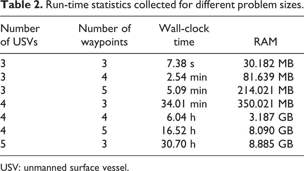
USV: unmanned surface vessel.

Multi-robot assembly case study

Mission modeling

We consider a multi-robot assembly comprising N assembly stations which allow human intervention when part assembly fails. Figure 4 shows an assembly cell. Each assembly station S_i has a dexterous mobile manipulator M_i . Two conveyor systems are also provided, $B_{1}$ is responsible for bringing parts from storage to assembly stations whereas $B_{2}$ is responsible for transferring parts among assembly stations. A pick-and-place robot P_i transfers parts from $B_{1}$ to station S_i .

Figure 4.

Schematic representation of multi-robot assembly cell.

Our convention is to denote by $n_{1}^{i}$ (superscript refers to an assembly station, and subscript is only a variable index) the number of parts arrived at S_i , and by $n_{2}^{i}$ the number of complete assemblies produced, and by $n_{3}^{i}$ the number of partially completed assemblies arrived. At assembly station S ₁, the number of parts obtained from $B_{1}$ is denoted by $n_{1}^{1}$ . The number of preliminary assemblies delivered by $B_{1}$ is denoted by $n_{3}^{1}$ . These units are then assembled to form subassemblies which will be transferred to station S ₂ via $B_{2}$ . The number of subassemblies produced at station S ₁ is denoted by $n_{2}^{1}$ . The number of subassemblies transferred from S ₁ to S ₂ is $n_{3}^{2}$ . Similarly, $B_{1}$ delivers parts from storage to station $A_{2}$ whose number is recorded as $n_{1}^{2}$ . The number of subassemblies produced here is $n_{2}^{2}$ . The number of these subassemblies transferred from S ₂ to S ₃ by $B_{2}$ is $n_{3}^{3}$ and the number of parts delivered by $B_{1}$ is $n_{1}^{3}$ . Finally, the number of parts produced at station S ₃ is $n_{2}^{3}$ .

The final assemblies produced at station S ₃ are either transferred by the conveyor system or another mobile robot for storage or sorting. At the start of operations, it is a common practice to have some parts in the stations (initial part buffer) so that assembly operations may start without initial bottlenecks. So let $n_{1}^{i} > 0$ . All other variables will be initially zero.

Now we describe the probabilistic transition model (see “Missions with probabilistic transitions” section) for assembly robots. Let us first consider model for robot M ₂ (Figure 5). The subassemblies arriving from the former assembly station undergo a pre-detection operation. For this, let us assume robot M ₂ to be a mobile bi-manipulator having a camera fixed to one of its arms. After pre-detection, the part is either sent for pre-repair if problems are detected or sent for the assembly process. Let us assume that the probability of success during pre-detection denoted by p ₁ is the same for all assembly stations. If pre-detection succeeds, then the number of parts available for assembly process denoted by $x_{2}^{2}$ is incremented by one, otherwise the number of parts which must be pre-repaired denoted by $x_{1}^{2}$ gets increased by one. When the robot performs the pre-repair operation, it may succeed with a probability of p ₂ and then queue up the part for the assembly process. Otherwise, it reports failure to repair the part based on sensory feedback.

Figure 5.

Probabilistic transition model for assembly robot.

There are two contingency buffers in station S ₂: $C_{1}^{2}$ and $C_{2}^{2}$ . These are used to store part assemblies that require external help. Let us assume it to be in the form of a human helper H ₂ assigned to the station. Those parts that fail the pre-repair process are sent to contingency buffer $C_{1}^{2}$ , and the number of units held in this buffer is recorded as $c_{1}^{2}$ . When the robot performs the assembly process, it may succeed with a probability p ₃ and then queue up the parts to undergo post-detection. However, assembly processes may be complex, and robots may fail. In that case, they will repeat the assembly process. The number of parts held for post-detection is given by $x_{3}^{2}$ . If post-detection succeeds with probability p ₄, then the part is declared as finished subassembly ready to be transferred to the next assembly station. Otherwise, the parts are sent for post-repair. When the post-repair operation succeeds with probability p ₅, then the assembly is declared as finished as per station S ₂. However, if post-repair fails, then the part is sent to contingency buffer $C_{2}^{2}$ . Human H ₂ is responsible for both the contingency buffers and attempts to resolve each unit held in these buffers. If human succeeds with probability p ₆ for the units held at $C_{1}^{2}$ , then they are queued up for assembly. If human succeeds with the units held at $C_{2}^{2}$ with the same probability, then they are declared as finished subassemblies ready for transport to the next assembly station.

Model for robot M ₃ is the same. Model for robot M ₁ is a simplified version of M ₂ because there are no operations like pre-detection and pre-repair, hence also no contingency buffer $C_{1}^{1}$ . Robot M ₁ directly performs its assembly operation followed by post-detection and post-repair operations. It must also be noted that all the container variables for stations $A_{2}$ and $A_{3}$ , namely $x_{1}^{i}, x_{2}^{i}, x_{3}^{i}, x_{4}^{i}, n_{1}^{i}, n_{2}^{i}, n_{3}^{i}, c_{1}^{i}, c_{2}^{i}$ for $i = 1, 2$ , and those for station $A_{1}$ , namely $x_{3}^{1}, x_{4}^{1}, n_{1}^{1}, n_{2}^{1}, n_{3}^{1}, c_{2}^{1}$ , represent storage of parts and naturally have size constraints associated with them. The lower bound for each is set to zero. The upper bounds also depend on whether we use numerical or statistical model-checking methods. If we use the numerical method, then our model size must be small, so we cannot have high upper bounds for these variables. Statistical methods give approximate results but accommodate larger model sizes.

We first define a base protocol on which the assembly process operates. The assembly process happens in cycles, each comprising multiple steps. In the first step of each cycle, conveyor brings parts from storage to different stations and also transfers parts among the different stations with probability p ₇ which we generally take to be 1 unless otherwise stated. PRISM only allows us to encode probabilistic transition rules to represent processes. So we must use the process-algebraic concept of synchronization supported in PRISM to simulate real operations. We model the three stations as separate modules which synchronize their processes with each other (see “Modeling of contingency resolution strategies” section). For example, we synchronize all transition rules corresponding to conveyor operations in the first step of each execution cycle.

In the next five steps, the assembly robots perform pre-detection, pre-repair, assembly, post-detection, and post-repair operations consecutively. In the seventh and eighth steps, the human helper at each station repairs parts in the two contingency buffers. The workers are not allowed to enter the station when assembly robots are operating. These cycles keep repeating until the size constraints on the variables allow to do so. We call this protocol strategy 1, which is modeled in PRISM simply as a DTMC. We define a reward structure (see “Model checking and verification” in the “Computational modeling” section) to compute the expected real-world time that elapses during assembly production. The conveyor operation is fast, but it still requires robots to transfer parts from the conveyor belts, so we assume it to take 0.2 min. The detection routines take 0.2 min also as scanning and processing of images may be sped up. The repair and assembly processes take 2 min. A human worker takes 5 min.

We could simulate the above assembly station to gather more insight. Suppose all buffer sizes are 4 and it produces five assemblies. In Figure 6(a), we show a random simulation run and assume all probabilities are one except p ₃ which is 70%. It takes 2.6 min to produce one assembly if events proceed without contingencies (this can immediately be checked based on the duration of the individual operations involved), but unexpected events occur such as an assembly failing to be produced successfully by the robot (such events are marked on the figure), and this increases the time taken to finish five parts. Thus, what could have been achieved in $2.6 \times 5 = 13$ min in the absence of contingencies now takes 24.2 min. In Figure 6(b), all probabilities are set to 70%. We denote the contingencies as and when they occur for a random simulation run. These disrupting events again explain the deviation from the nominal behavior. Since the probability of failure is higher across the assembly operations involved, it takes even higher time than before, that is, 31.8 min.

Figure 6.

Simulation of an assembly station. PRF: pre-repair failure; PDF: pre-detection failure; H: human worker succeeds in resolving faulty subassembly. (a) Assembly station with lower probability of failures. (b) Assembly station with higher probability of failures.

We also design a nondeterministic version of this protocol referred to as strategy A, which will be implemented as an MDP in PRISM. The first step remains the same. In the second step, the assembly robots perform one of their detection actions taking a maximum of 0.2 min. In the third step, the assembly robots perform one of their assembly/repair actions taking a maximum of 2 min. In the fourth step, human helper repairs parts in one of the contingency buffers requiring 5 min.

Model checking and verification

We first analyze a single assembly station. All variables are given an upper bound of four, and we wish to compute the expected time to produce 10 assemblies. And the initial part buffer is zero for each station. An assembly cell is perfect if all success probabilities are one. The expected production time for a perfect cell is the lowest bound achievable for the given transition system. These values are 26 and 26.12 min for strategies 1 and A, respectively. Let us assume that human succeeds with 95% probability and assembly robots with 80%. From Table 3, we see that increasing initial part buffer decreases expected production time by more than 30 s for both strategies 1 and A which is very significant for factory throughput in the long run. We observe that the nondeterministic station shows a decrease of 0.2 min per row because the addition of one item in the initial buffer helps skip one conveyor operation. This effect is not so vividly noticeable in the DTMC version. Increasing contingency buffer size does not have any notable effect. But increasing human success probability from 60% to 100% significantly reduces time for both strategies (Table 4). This analysis method may also be used as a recruitment tool. Suppose a fast worker could finish resolving contingencies in 5 min and an expert worker could succeed with a probability of 99%. Let a slow worker take 7 min and a less skilled worker succeed with a probability of 80%. Then we record the expected production times for all four combinations of worker in Table 5 for strategies 1 and A. We see that for both strategies, being slow is undesirable regardless of whether the worker is expert or less skilled. However, interestingly, if the slow worker were to take 6 min, then the slow and expert worker becomes preferable over the fast and less skilled worker. Such counterintuitive observations may differ for different mission parameters. Above results were generated via numerical model checking.

Table 3.

Effect of initial part buffer on production time.

Initial part buffer	Strategy 1Production time (in min)	Strategy A Production time (in min)
0	45.17	43.10
1	45.07	42.90
2	44.93	42.70
3	44.75	42.50
4	44.55	42.30

Table 4.

Effect of contingency resolution probability on production time.

Contingency resolution probability	Strategy 1Production time (in min)	Strategy A Production time (in min)
0.60	47.52	45.43
0.70	46.64	44.56
0.80	45.96	43.88
0.85	45.67	43.59
0.90	45.41	43.33
0.95	45.17	43.10
1.00	44.96	42.89

Table 5.

Effect of human characteristics on production time.

Contingency resolution probability	Contingency resolution duration (in min)	Expected production time (in min)
Contingency resolution probability	Contingency resolution duration (in min)	Strategy 1	Strategy A
0.99	5	45.01	42.93
	6	45.86	43.71
	7	46.72	44.50
0.80	5	45.96	43.88
	6	47.00	44.84
	7	48.05	45.79

The problem with analyzing multi-station assembly cells as MDPs is state space explosion which makes model building, as well as model checking, very memory-intensive and time-consuming, if not impossible. However, the DTMC protocol of strategy 1 may be extended to multi-station assembly cells and analyzed using PRISM’s simulation-based model-checking techniques. We first consider a two-station cell by ignoring station S ₃. All variables are given an upper bound of two, and we wish to compute the expected time to produce three assemblies. And the initial part buffer is one for each station. The expected production time for a perfect cell is 10.2 min.

Now let human succeed with 95% probability, robot assembly with 90%, and other operations with 80%. We compare the expected production time of strategy 1 with four other strategies in Figure 7 and the time is shown as the percentage increase with respect to that of the perfect cell. We run the simulation 100 times to report statistics at 95% confidence level, a width of 0.5 min, and the maximum path length of a billion states. Strategy 2 is designed assuming only one human is available for the entire cell who alternates between both the stations in odd and even cycles. Strategy 3 is the same as 1, but the humans at each station must resolve the first contingency buffer in odd cycles and the second one in even cycles. Strategy 4 again assumes only one human for the entire cell, but he or she succeeds in resolving contingencies with 80% probability, fails and puts the part back in the buffer with 5% probability, and sends the part for repair by the robot with 15% probability. This simulates the behavior of a human who reckons that a minor fix could help the robot assemble the part on its own, so he or she sends the parts back to the automated assembly cell. For example, a human decides that if a washer is slightly tweaked, then the assembly robot will succeed with the rest of the assembly. Thus, this human worker may be assumed to be faster and spend only 2 min. Strategy 5 is the same as 4 but with one human per station. Now it is not obvious which strategy will be the best. These comparison results help us analyze time savings that can be achieved for manufacturing operations which may help make huge profits in the long run. We see that on an average strategy 5 performs the best but only marginally better than strategy 4. Strategy 2 shows significant improvement over strategy 1 on account of using only one human to balance the task of two humans efficiently. However, when the two humans organize themselves better as in strategy 3, then they outperform strategy 2 by a small margin.

Figure 7.

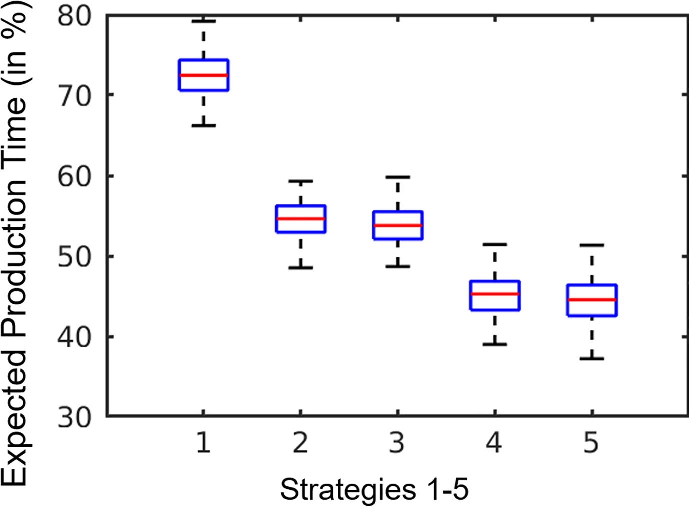
Effect of different strategies on expected production time.

We compare these strategies only for two-station cells because model checking for strategies 2, 3, and 4 becomes time-consuming for three-station cells. This is because these strategies require coding more steps per cycle and handling of both conveyor systems triggers scaling issues.⁴⁵ PRISM run-time statistics illustrate these issues clearly. Model construction for two stations with strategy 2 took 1.9 s, having around 4.3 million states and 6.5 million transitions. Statistical model checking took 0.14 s. But model construction for three stations with strategy 2 took 21.4 s and verification took 2.1 s.

Consider the three-station assembly cell operating with strategy 1 and the same variables upper bounds and initial part buffer as before. If all success probabilities within a station are at 90%, we call it a low station. High stations have success probabilities at 99%. The conveyor system is assumed to be operating perfectly. A perfect cell takes 12.8 min. In Figure 8(a), we plot the expected production time as the percentage increase with respect to that of the perfect cell for all $2^{3}$ combinations of high and low stations in the cell. For example, LHL on x-axis denotes that the first and third stations are low, and the second one is high. We observe that the first station being low is not as critical as the next two stations being low. We see a similar trend for strategy 5 (letting human helper three-way split still be 80-15-5) in Figure 8(b). We also observe that at these high probabilities for the three-station assembly cell, both strategies start performing similarly.

Figure 8.

Effect of different combinations of stations on expected production time: (a) strategy 1 and (b) strategy 5.

Modeling of large-scale assembly operations

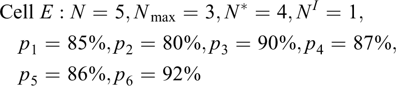
Imagine a production line which is composed of several assembly cells to produce a complex product such as a satellite. Such a product would have to be assembled across a number of assembly cells, and it is not possible to model and analyze the entire assembly operation in PRISM in one go because of the memory overflow problem. We can, however, break the entire assembly line down to its cellular level and analyze each of the cells separately as in “Model checking and verification” in the “Multi-robot assembly case study” section. Thereafter, we can aggregate the results of these individual analyses to figure out how contingencies can be handled. We shall demonstrate how our approach can be scaled up for larger problem sizes. Suppose there are five assembly cells as shown in Figure 9 with the specifications given below

Figure 9.

Scenario for multiple assembly cells interacting with each other.

Cell A : N = 2, N_{max} = 3, N^{*} = 4, N^{I} = 2, p_{1} = p_{2} = p_{3} = p_{4} = p_{5} = 90 %, p_{6} = 95 %

Cell B : N = 3, N_{max} = 2, N^{*} = 5, N^{I} = 0, p_{2} = 85 %, p_{3} = 90 %, p_{4} = 95 %, p_{1} = p_{5} = p_{61} = 80 %, p_{62} = 5 %, p_{63} = 15 %

Cell C : N = 2, N_{max} = N^{*} = N^{I} = 3, p_{2} = p_{3} = p_{4} = 90 %, p_{1} = p_{5} = 95 %, p_{61} = 80 %, p_{62} = 5 %, p_{63} = 15 %

Cell D : N = 3, N_{max} = 2, N^{*} = 3, N^{I} = 0, p_{1} = p_{5} = 85 %, p_{2} = p_{4} = 80 %, p_{3} = p_{6} = 90 %

Cell E : N = 5, N_{max} = 3, N^{*} = 4, N^{I} = 1, p_{1} = 85 %, p_{2} = 80 %, p_{3} = 90 %, p_{4} = 87 %, p_{5} = 86 %, p_{6} = 92 %

Let the initial part buffer be constant N^I for each cell. The upper bound for all other storage buffers of a cell is $N_{max}$ , and it can produce a maximum of $N^{*}$ assemblies. The arrows represent the direction in which assemblies will transfer from one cell to another. Suppose we want to improve upon the strategies being executed at each cell. We use MATLAB to generate PRISM scripts for each cell for the above parameter values. Let us assume that the initial strategies for each cell are $(A,3), (B,5), (C,5), (D,2), (E,3)$ .

According to Figure 9, cells A and B begin their production initially and feed subassemblies to cell C. So we can analyze cell C separately from the other cells due to this nature of interactions between the cells. And later on, we could compute the overall performance based on the above interactions.

The automated case-by-case analysis in MATLAB then reasons as follows: Cell A takes 4.475 min and cell B takes 5.894 min per assembly produced. Cell B's strategy is optimal. However, cell A employs two humans and strategy 3. So we could find another strategy where fewer humans are employed even if this results in worsening of cell A's production time as long as it does not overshoot 5.894 min. This is because cell C would not be able to proceed unless parts arrive from both cells A and B. If cell A switches to strategy 2, then it employs only one human, and so brings down the operational costs; it takes 4.482 min.

Similarly, cells C and D must feed parts to cell E, but cell C takes 4.406 min and cell D takes 8.115 min per part. Cell C's strategy is optimal and requires two humans. Switching to strategies requiring fewer humans does not increase its production time. However, it may still be profitable to switch to a strategy that requires fewer workers. Additionally, we may bring down cell D's production time without adding humans. If cell D switches to strategy 4, it brings down the production time to 7.673 min. Since cell E is the last cell, we choose its optimal strategy independent of any other factor. Thus, we analyzed a production line of 15 assembly cells by embedding the probabilistic model checker within a higher level MATLAB simulation.

Conclusion and future work

We present a framework that allows us to do modeling of nominal missions with deterministic and probabilistic transitions. We also demonstrate the modeling of contingency resolution strategies with specific examples of contingencies for two case studies. Existing model checkers are used to evaluate these strategies. In the first case study, we verify the correctness of contingency resolution strategies and use NuSMV to generate mission execution plans for different scenarios. In the second case study, we use PRISM as a computational tool to provide a probabilistic assessment for mission success and analyze the effect of relevant mission variables on mission execution.

We plan to examine the robustness and completeness of our modeling and verification techniques using a detailed model of assembly line created from physical experiment data. This shall help us improve our model as well as record the performance of integrating model checkers in real-time missions for proactive contingency handling compared to existing reactive techniques. We aim to integrate high-fidelity simulation software packages with model checkers because the former are good at analyzing the performance and behavior of agents at a finer level of detail. Rather than running exhaustive and full-fledged simulations, we may use the model checking results to simulate fewer small-sized cases. We shall also deploy machine learning algorithms so that newer and better contingency resolution strategies are automatically generated based on sensory feedback and the history of human interventions. This shall be very effective for scenarios where contingencies occur at high frequencies amid rapidly changing mission conditions.

Footnotes

Declaration of conflicting interests

The author(s) declared no potential conflicts of interest with respect to the research, authorship, and/or publication of this article.

Funding

The author(s) disclosed receipt of the following financial support for the research, authorship, and/or publication of this article: This work was supported by National Science Foundation Grant no. 1634433. Opinions expressed are those of the authors and do not necessarily reflect the opinions of the sponsors.

ORCID iD

Shaurya Shriyam

Satyandra K Gupta

References

Pogromsky

Adriaansen

, et al. A control of collision and deadlock avoidance for automated guided vehicles with a fault-tolerance capability. Int J Adv Robot Syst 2016; 13(2): 64.

Shriyam

Shah

Gupta

. Decomposition of collaborative surveillance tasks for execution in marine environments by a team of unmanned surface vehicles. J Mech Robot 2018; 10(2): 025007.

Ardiny

Witwicki

Mondada

. Construction automation with autonomous mobile robots: a review. In: Proceedings of RSI international conference on robotics and mechatronics (ICROM), Tehran, Iran, 7–9 October 2015, pp. 418–424. IEEE.

Malhan

Kabir

Shembekar

, et al. Hybrid cells for multi-layer prepreg composite sheet layup. In: Proceedings of IEEE international conference on automation science and engineering (CASE), Munich, Germany, 20–24 August 2018, pp. 1466–1472. IEEE.

Malhan

Kabir

Shah

, et al. Automated prepreg sheet placement using collaborative robotics. In: Proceedings of SAMPE technical conference and exhibition 2018, Long Beach, CA, USA, 21–24 May 2018. SAMPE.

Bhatt

Kabir

Malhan

, et al. A robotic cell for multi-resolution additive manufacturing. In: Proceedings of IEEE international conference on robotics and automation (ICRA), Montreal, Canada, 20–24 May 2019, pp. 2800–2807. IEEE.

Bhatt

Kabir

Peralta

, et al. A robotic cell for performing sheet lamination-based additive manufacturing. Addit Manuf 2019; 27: 278–289.

Cimatti

Clarke

Giunchiglia

, et al. NuSMV 2: an opensource tool for symbolic model checking. In: Proceedings of international conference on computer aided verification, Copenhagen, Denmark, 27–31 July 2002, pp. 359–364. Springer.

Kwiatkowska

Norman

Parker

. Prism 4.0: verification of probabilistic real-time systems. In: Proceedings of international conference on computer aided verification, Berlin, Heidelberg, 14 July 2011, pp. 585–591. Springer.

10.

Sheshkalani

Khosravi

. Verification of visibility-based properties on multiple moving robots in an environment with obstacles. Int J Adv Robot Syst 2018; 15(4): 1729881418786657.

11.

Winfield

Fernández-Gago

, et al. On formal specification of emergent behaviours in swarm robotic systems. Int J Adv Robot Syst 2005; 2(4): 39.

12.

Bolton

Bass

Siminiceanu

. Using formal verification to evaluate human-automation interaction: a review. IEEE Trans Syst Man Cybern 2013; 43(3): 488–503.

13.

Pant

Abbas

Quaye

, et al. Fly-by-logic: control of multi-drone fleets with temporal logic objectives. In: Proceedings of the 9th ACM/IEEE international conference on cyber-physical systems, Porto, Portugal, 11–13 April 2018 pp. 186–197. Piscataway, NJ, USA: IEEE Press.

14.

Liu

Dai

, et al. Distributed communication-aware motion planning for multi-agent systems from STL and SpaTeL specifications. In: Proceedings of IEEE conference on decision and control (CDC), Melbourne, VIC, Australia, 12–15 December 2017, pp. 4452–4457. Piscataway, NJ, USA: IEEE Press.

15.

Nikou

Boskos

Tumova

, et al. Cooperative planning for coupled multi-agent systems under timed temporal specifications. In: Proceedings of IEEE American control conference (ACC), Seattle, WA, USA, 24–26 May 2017, pp. 1847–1852. IEEE.

16.

Zhou

Maity

Baras

. Optimal mission planner with timed temporal logic constraints. In: Proceedings of IEEE European control conference (ECC), Linz, Austria, 15–17 July 2015, pp. 759–764. IEEE.

17.

Fraser

Wotawa

Ammann

. Testing with model checkers: a survey. Softw Test Verif Rel 2009; 19(3): 215–261.

18.

Fainekos

Girard

Kress-Gazit

, et al. Temporal logic motion planning for dynamic robots. Automatica 2009; 45(2): 343–352.

19.

Lahijanian

Wasniewski

Andersson

, et al. Motion planning and control from temporal logic specifications with probabilistic satisfaction guarantees. In: Proceedings of IEEE international conference on robotics and automation (ICRA), Anchorage, AK, USA, 3–7 May 2010, pp. 3227–3232. IEEE.

20.

Finucane

Jing

Kress-Gazit

. LTLMoP: experimenting with language, temporal logic and robot control. In: Proceedings of IEEE/RSJ international conference on intelligent robots and systems (IROS), Taipei, Taiwan, 18–22 October 2010, pp. 1988–1993. IEEE.

21.

Konur

Dixon

Fisher

. Analysing robot swarm behaviour via probabilistic model checking. Robot Auton Syst 2012; 60(2): 199–213.

22.

Miyawaki

Masamune

Suzuki

, et al. Scrub nurse robot system-intraoperative motion analysis of a scrub nurse and timed-automata-based model for surgery. IEEE Trans Ind Electron 2005; 52(5): 1227–1235.

23.

Van

Fredivianus

Tran

, et al. Formal verification of ALICA multi-agent plans using model checking. In: Proceedings of the ninth international symposium on information and communication technology, Danang City, Vietnam, 6–7 December 2018, pp. 351–358. ACM.

24.

Marinescu

Seceleanu

, et al. Formal verification of an autonomous wheel loader by model checking. In: Proceedings of IEEE/ACM international FME workshop on formal methods in software engineering (FormaliSE), Gothenburg, Sweden, 27 May–3 June 2018, pp. 74–83. IEEE.

25.

Karaman

Frazzoli

. Linear temporal logic vehicle routing with applications to multi-UAV mission planning. Int J Robust Nonlin 2011; 21(12): 1372–1395.

26.

Guo

Dimarogonas

. Task and motion coordination for heterogeneous multiagent systems with loosely coupled local tasks. IEEE Trans Autom Sci Eng 2017; 14(2): 797–808.

27.

Schillinger

Bürger

Dimarogonas

. Simultaneous task allocation and planning for temporal logic goals in heterogeneous multi-robot systems. Int J Robot Res 2018; 37(7): 818–838.

28.

Shoukry

Nuzzo

Balkan

, et al. Linear temporal logic motion planning for teams of underactuated robots using satisfiability modulo convex programming. In: Proceedings of IEEE conference on decision and control (CDC), Melbourne, VIC, Australia, 12–15 December 2017, pp. 1132–1137. IEEE.

29.

Kamali

Dennis

McAree

, et al. Formal verification of autonomous vehicle platooning. Sci Comput Program 2017; 148: 88–106.

30.

Machin

Guiochet

Waeselynck

, et al. SMOF: a safety monitoring framework for autonomous systems. IEEE Trans Syst Man Cybern 2018; 48(5): 702–715.

31.

Thrun

Burgard

Fox

. Probabilistic robotics. Cambridge: MIT press, 2005.

32.

Liu

Cong

Zou

, et al. A biological-inspired episodic cognitive map building framework for mobile robot navigation. Int J Adv Robot Syst 2017; 14(3). https://doi.org/10.1177/1729881417705922.

33.

Jiang

Kumar

. Diagnosis of repeated failures for discrete event systems with linear-time temporal-logic specifications. IEEE Trans Autom Sci Eng 2006; 3(1): 47–59.

34.

Chatterjee

Chmelk

Gupta

, et al. Qualitative analysis of POMDPs with temporal logic specifications for robotics applications. In: Proceedings of IEEE international conference on robotics and automation (ICRA), Seattle, WA, USA, 26–30 May 2015, pp. 325–330. IEEE.

35.

Lacerda

Parker

Hawes

. Optimal and dynamic planning for Markov decision processes with co-safe LTL specifications. In: Proceedings of IEEE/RSJ international conference on intelligent robots and systems (IROS), Chicago, IL, USA, 14–18 September 2014, pp. 1511–1516. IEEE.

36.

Cizelj

Ding

Lahijanian

, et al. Probabilistically safe vehicle control in a hostile environment. Presented at World Congress of the International Federation of Automatic Control (IFAC), Milano, Italy, 28 August–2 September 2011, pp. 11803–11808.

37.

Ding

Smith

Belta

, et al. Optimal control of Markov decision processes with linear temporal logic constraints. IEEE Trans Autom Control 2014; 59(5): 1244–1257.

38.

Faruq

Lacerda

Hawes

, et al. Simultaneous task allocation and planning under uncertainty. In: Proceedings of IEEE/RSJ international conference on intelligent robots and systems (IROS), Madrid, Spain, 1–5 October 2018, pp. 3559–3564. IEEE.

39.

Feng

Wiltsche

Humphrey

, et al. Synthesis of human-in-the-loop control protocols for autonomous systems. IEEE Trans Autom Sci Eng 2016; 13(2): 450–462.

40.

Kloetzer

Mahulea

. LTL-based planning in environments with probabilistic observations. IEEE Trans Autom Sci Eng 2015; 12(4): 1407–1420.

41.

Chen

Tumová

Belta

. LTL robot motion control based on automata learning of environmental dynamics. In: Proceedings of IEEE international conference on robotics and automation (ICRA), Saint Paul, MN, USA, 14–18 May 2012, pp. 5177–5182. IEEE.

42.

Kwiatkowska

Norman

Parker

. Stochastic model checking. In: Proceedings of international school on formal methods for the design of computer, communication and software systems, Bertinoro, Italy, 28 May–2 June 2007, pp. 220–270. Springer.

43.

Martins

Al Tair

Santos

, et al. αPOMDP: POMDP-based user-adaptive decision-making for social robots. Pattern Recogn Lett 2019; 118: 94–103.

44.

Shriyam

Gupta

. Incorporating potential contingency tasks in multi-robot mission planning. In: Proceedings of the IEEE international conference on robotics and automation (ICRA), Brisbane, Australia, 21–25 May, pp. 1–7. IEEE.

45.

Shriyam

Gupta

. Modeling and analysis of subsystem interactions in robotic assembly. In: Proceedings of ASME international design engineering technical conferences and computers and information in engineering conference, Anaheim, California, USA, 18–21 August 2019. ASME.

Modeling and verification of contingency resolution strategies for multi-robot missions using temporal logic

Abstract

Keywords

Introduction

Literature review

Formal modeling of multi-robot missions

Model checkers for mission verification

Handling stochastic events

Description of framework

Overview

Mission abstraction

Formal representation

Missions with deterministic transitions

Missions with probabilistic transitions

Computational modeling

Modeling of contingency resolution strategies

Model checking and verification

Multi-USV case study

Mission modeling

Model checking and verification

Multi-robot assembly case study

Mission modeling

Model checking and verification

Modeling of large-scale assembly operations

Conclusion and future work

Footnotes

Declaration of conflicting interests

Funding

ORCID iD

References