Magnetohydrodynamic velocity profile measurement for microelectromechanical systems micro-robot design

Abstract

The development of microelectromechanical systems based on magnetohydrodynamic for micro-robot applications requires precise control of the micro-flow behavior. The micro-flow channel design and its performance under the influence of the Lorentz force is a critical challenge, the mathematical model of each magnetohydrodynamic device design must be experimentally validated before to be employed in the fabrication of microelectromechanical systems. For this purpose, the present article proposes the enhancement of a particle image velocimetry measurement process in a customized machine vision system. The particle image velocimetry measurements are performed for the micro-flow velocity profile mathematical model validation of a magnetohydrodynamic stirrer prototype. Data mining and filtering have been applied to a raw measurement database from the customized machine vision system designed to evaluate the magnetohydrodynamic stirrer prototype. Outlier’s elimination and smoothing have been applied to raw data to approximate the particle image velocimetry measurements output to the velocity profile mathematical model to increase the accuracy of a customized machine vision system for two-dimensional velocity profile measurements. The accurate measurement of the two-dimensional velocity profile is fundamental owing to the requirement of future enhancement of the customized machine vision system to construct the three-dimensional velocity profile of the magnetohydrodynamic stirrer prototype. The presented methodology can be used for measurement and validation in the design of microelectromechanical systems micro-robot design and any other devices that require micro-flow manipulation for tasks such as stirring, pumping, mixing, networking, propelling, and even cooling.

Introduction

The most common industrial and civil applications that use robots for automation are the automotive industry, food industry, and manufacturing industries of diverse products, to mention some. The sizes of those kinds of robots are on an adequate scale for human handling. Most of those robots can navigate, can perform inspections for the identification and measurement of diverse magnitudes through sensors that simulate the tactile and visual human senses, and also can transport materials and/or products from one place to another. Some robots are static on a place; others navigate in different ways, that is, terrestrial, aerial, underwater, and even in the space, while other robots can navigate within the human body. ¹

Some special applications require micro-robots, such as micromachining process, the electrical testing process through microprobes, micro-pumping, micro-mixing, and a lot of biomedical, biological, and environmental applications including drug delivery, biomedical assays, microfluidics analyses, cell culturing, micro-assembly, micro-surgery, micro-manipulation, and others. ² All of these applications have been benefited with the advances in technologies in the last two decades, especially with the development of microelectromechanical systems (MEMS) for a wide range of different functions, among which stands out the microfluidic devices, such as stirring, pumping, mixing, networking, propelling, and even cooling.

The need for measuring the velocity of flowing stream in fluidic channels has given the origin to the particle image velocimetry (PIV) technique. In the beginning, the first velocity flow measurements were done tracking the trajectory of debris over the flow surfaces of natural channels, such as rivers. With the development of the mechanics of fluids and the innovation in the use of fluids and microfluidics for a lot of applications, it was necessary to seed particles in the fluid and develop a technique to track their trajectory, measure their velocity, and define its moving patterns, in order to obtain an accurate, quantitative measurement of fluid velocity vectors at a very large number of points simultaneously. ³ Besides due to the development of computers, sophisticated machine vision systems for PIV have been designed for different applications, where the PIV technique challenge and complexity depend on the characteristics of the application as well as on the required resolution and accuracy. Examples of systems that use the PIV techniques to characterize its performance are the turbulent jets used in a wide variety of applications, as in marine propulsion, pollutant discharge, or studies on the cardiocirculatory system. ⁴ The turbines are used for hydropower purposes to analyze from complex turbulent to two-phase flows. ⁵ Centrifugal pumps are used to measure the complex flow structures around the volute tongue region, where intense rotor–stator interaction appears. ⁶ Solid–liquid laminar stirrer tank with floating particles is used for industrial processes, such as the production processes of coatings, cosmetics, and lubricating oil. ⁷ And microfluidics in annular channels for MHD stirrers. ⁸

Since micro-applications started to develop and surged the need for propelling, stirring, and control flows to perform tasks such as mixing and networking at micro-scale, prototypes based on the principle of magnetohydrodynamics (MHD) have been considered. ⁹ MHD prototypes enable fluid manipulation for tasks such as pumping, networking, propelling, stirring, mixing, and even cooling without the need for mechanical components, its nonintrusive nature provides a solution to mechanical systems issues. The lack of mechanical elements reduces the possibilities of breakdowns, undesired vibrations, and noise. MHD is particularly useful for microfluidic applications where a conductive fluid needs to be manipulated to perform specific operations. The most common applications of MHD are micro-pumping (in lab-on-a-chip (LOC’s) and liquid chromatography), ^10,11 networking (in LOC’s), ¹² stirring and mixing (in LOC’s, polymerase chain reaction, and chemical reactors), ^{13 –15} micro-cooling (in microelectronics), and thermal cyclers. ¹⁶

However, the design of MHD prototypes is not an easy task. The design requires a precise flow control, which depends on several parameters, like microfluidics conductivity, microfluidics channel shape and size configuration, and the interaction between electric and magnetic fields. All these parameters and others are included in the mathematical model of an MHD stirrer prototype proposed.

The present article describes the accurate mathematical model validation of an MHD stirrer prototype. It also presents a technique for the enhancement of a PIV measurement process for a customized machine vision system developed for the proposed MHD stirrer prototype model validation. Previous measurement experimentation has been done with this customized system, but on that occasion only measuring the maximum velocity from the free surface of a three-dimensional (3-D) velocity profile was validated, see the study by Valenzuela-Delgado et al. ¹⁷ As stated in that previous publication, the objective for future work is to modify the MHD stirrer prototype to introduce a laser sheet to measure the 2-D velocity profiles at different planes, to experimentally recreate the 3-D velocity profile. However, for the next step for further work, in this article, the 2-D velocity profile of the free surface is accurately validated.

As a strategy to increase the mathematical model validation accuracy, the technique developed for the enhancement of a PIV measurement process includes the use of data mining methods and filtering. PIV can be classified as a data stream application, which can be benefited from data mining and filtering. This involves the elimination of outliers from the data set and data smoothing. Due to the nature of MHD stirrer, the microfluidic velocity measurement can provide a nonstationary distribution of data that require to be updated to the measurement system to ensure stability in its performance. Basically, it is accomplished by learning from a set of PIV instances gathered along the data stream, also known as batch-incremental learning. ¹⁸

Data mining and filtering are frequently used to contribute to the accuracy improvement of systems from different technologies and applications. As has been demonstrated ^19,20,21 , also for Optical Scanning Systems where measurements error due to motor eccentricity have been decreased. Also demonstrated ²² for medical devices that were malfunctioning due to electrostatic occurrence that could be identified thanks to the data processing of a big dataset of failures. The same regarding Malware detection although of its complex nature and it’s quickly changing and therefore turn out to be harder to recognize ²³ , and an endless list of data mining and filtering examples could be mentioned. Few researchers’ publications are identified as fusion of data mining, filtering, and PIV topics, but some work has been done, for example, developing of a generic seeding generator for other researchers investigating the production of aerosols for PIV application which has been enhanced by a simple model for the prediction of the droplet size mean diameter. ²⁴ A computational study of the flow from a set of three-stream jets has been based on the noise predictions using an acoustic analogy-based method whose sound source model was calibrated for a baseline shear stress transport solution. ²⁵ A 3-D three-component database for time series of velocity field measured by tomographic time-resolved PIV was data mining using the quadrant splitting method, which is used to detect and extract the inherent coherent structures from turbulence signal database and to investigate the spatial topologies of fluctuating velocity and fluctuating vorticity. ²⁶ An artificial neural network was used to analyze the performance of data in phase Doppler anemometry and PIV which can measure droplet size and velocity in combustion spray for a practical combustion burner. ²⁷ By another side, some research ²⁸ proposed an adaptation of the median test for the detection of outliers in PIV data demonstrating that normalized median test yields a more or less “universal” probability density function for the residual and that a single threshold value can be applied to effectively detect outlier’s data. While research ²⁹ proposes variable threshold outlier identification and cellular neural network techniques, and research ³⁰ proposes an all-in-one method (discrete cosine transform (DCT)–penalized least squares (PLS)), based on a PLS approach, combines the use of the DCT and the generalized cross-validation, thus allowing fast unsupervised smoothing of PIV data.

About the proposed MHD model validation, raw data have been submitted to outlier’s elimination and smoothing. The obtained results have been fed as feedback to the measurement process to approximate the results from the customized PIV measurement system to the velocity profile mathematical model. The presented technique can be used in the design of MEMS micro-robot design and for any devices based on fluids. With the enhancement of the PVI technique proposed, the required customized machine vision systems for 3-D micro-flow measurement of MEMS micro-robots can be instrumented to (a) improve the design of MEMS micro-robots by supporting the validation of the mathematical model and to the selection of the values of main parameters involucrate in the MEMS micro-robots design and production process (flow conductivity, channel size and shape, Lorentz force value, electrodes configuration, etc.) and (b) verify each process of the production of the MEMS micro-robots and their final functionality, quality, and reliability.

MEMS-based on MHD for micro-robot applications

The main micro-robot applications are related to MEMS based on microfluidic devices manipulated by electromagnetic actuation, such as therapeutic drugs ³¹ and cells delivery micro-robots, ³² bacterial micro-robots for guiding, mixing, and killing pathogens for targeted therapy, ³³ cell manipulation, micromanipulation, and medical imaging, while micro-robots navigate in small-scale aqueous environments and for selective isolation of particles from a solution. ³⁴

Micro-robotics systems sizes are in the order of millimeters and centimeters due to they are systems integrated by subsystems such as power supply, sensors, actuators, locomotion, communication, control, and tool modules ³⁵ , while MEMS are in the order of microns. The majority of micro-robots have been produced using techniques such as 3-D printing, micro-molding, or with the aid of laser machining systems; also other fabrication methods consist of the use of standard photolithography to pattern robots using photoresist with embedded magnetic particles. ³⁶ Micro-robots might be categorized based on their principle of functioning (piezoelectric, electromagnetic, photoresists, and thermal), structure, dimensions (linear or planar), mobile or stationary, and applications. ³⁷

The major challenge during the design and fabrication of micro-robots development is the actuation due to their small size. So, a large power source cannot be useful for micro-robots, and other alternatives actuation methods, such as piezoelectric actuators, bacterial actuators, swimming tail actuator, and electromagnetic actuators, had been looked for. The electromagnetic actuators show an advantage over another kind of actuators. The electromagnetic field enables precise control of magnetic objects by controlling a current, so microfluidics can be handled by the Lorentz force. Consequently, many electromagnetic-driven micro-robots have been studied. ³⁸

Some MEMS based on electromagnetics can act as efficient actuators integrating magnetostrictive thin films into mechanical devices, and magnetic energy can be directly converted into mechanical energy; moreover, they can be remotely controlled, they present low-performance degradation, and its response time can be considered as fast as semiconductors. ³⁹ But some other MEMS based on electromagnetics and microfluidics are driven by the Lorentz force, by that reason can be called MEMS based on MHD, where the interaction between the magnetic and electric field induces a micro-fluidic behavior, which can be manipulated for specific purposes. ⁴⁰

MHD stirrer

The MHD stirrer under evaluation is an annular open channel driven by a Lorentz force acting in an electrically conductive solution, during the presence of electric and magnetic fields. An annular duct formed by two concentric electrically conducting cylinders limited by an insulating bottom wall. The annular channel is centered in a neodymium permanent magnet, inducing a uniform magnetic field parallel to the axes of the cylinders, along the vertical direction. When a ϕ voltage is applied between the cylindrical electrodes of copper, a radial electric current arises in the conducting fluid. The produced azimuthal Lorentz force drives the flow by the interaction of the radial current with the axial magnetic field, generating the distributed body force on the fluid, and circulating a fluid continuously in a closed loop to form a conduit with a virtual infinite length. The microfluid used is distilled water mixed with 10 nm seeding particles covered with silver-coated hollow glass sphere (S-SHGS; Dantec Dynamics seeding particles) that makes water electrically more conductive and less vulnerable to bubble generation and electrode oxidation. As the fluid has uniform electric conductivity, mass density, and kinematic viscosity, it allows them to propel without inducing a change in the applied electric field. By consequence obtaining a microfluidic velocity behavior uncoupled from potential difference and an induced current that does not add drag forces that could affect the configuration of the flow.

In the governing mathematical model, the 3-D steady laminar flow is analyzed taking into account the effect of the walls. Walls provide a type of friction, which produces a fluid resistance, commonly called drag force. Drag forces act opposite to the fluid motion; they can appear on fluid surfaces with a magnitude proportional to the velocity of laminar flow. The effect of the three walls is analyzed in detail by considering the gap between the cylinders as well as the depth of the channel. The developed mathematical governing model expressed in equation (1) was solved for the velocity steady flow quasi-analytic approximation by a Galërkin method with orthogonal Bessel–Fourier series, where $v_{\theta }$ is the approximating solution for azimuthal velocity, ${\alpha }_m$ is the mth Bessel eigenvalue, g_n is the nth constant Galërkin coefficient, v is the kinematic viscosity, R ₁ is the electrode internal radio, R ₂ is the electrode external radio, r is the distance from R ₁ and R ₂, $\eta =R_1/R_2$ , h is the channel depth, and $\epsilon =h/R_2$ is the aspect ratio. For details of the mathematical model see Valenzuela-Delgado et al. ¹⁷ Mathematical model computing results are shown in Figure 1, where r is the distance from R ₁ and R ₂, and $v_{\theta }$ is the flow velocity, and the red line over the free surfaces represents the 2-D velocity profile

$v_{\theta }={\displaystyle \sum }_{m=1}^M{\displaystyle \sum }_{n=1}^N\frac{8{\left(-1\right)}^{n+1}{\alpha }_m}{\left({\alpha }_m^2+\frac{{\left[\left(2n-1\right)\pi \right]}^2}{4{\epsilon }^2}\right)\left(v_{1;m}^{´2}\left(1\right)-{\eta }^2{v}_{1;m}^{´2}\left(\eta \right)\right)|\text{ln}\eta |}\frac{v_{0;m}^{}\left(1\right)-v_{0;m}^{}\left(\eta \right)}{\left[\left(2n-1\right)\pi \right]}{v}_{1,m}\left(r\right)g_n\left(z\right)$

1

Figure 1.

MHD stirrer. (a) Annular channel and (b) tilt view of the free surface with the 2-D velocity profile. MHD: magnetohydrodynamic.

Machine vision system for MHD stirrer model validation

The machine vision system to measure the velocity profile is integrated into the designed MHD stirrer. It contains an illumination subsystem and a camera mounted on a mobile arm over the stirrer. ⁴¹ Due to the transparency of the fluid to explore its behavior through the machine vision system, it has been doped with a high density (forming speckles) of S-SHGSs, borosilicate glass spheres with a smooth and reflectivity surface due to a thin silver coating (also enable the electrical conductivity), see Figure 2.

Figure 2.

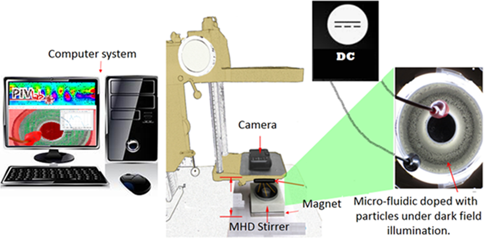
Customized machine vision system for MHD stirrer. MHD: magnetohydrodynamic.

The control of the illumination level and the lighting direction play an important role in the video recording performance. By this reason, the free surface of the stirrer flow is illuminated with an LED ring wrapped in a diffuser to obtain a darkfield illumination phenomenon to avoid undesirable light reflection. This kind of illumination provides a high contrast image due to the light is guided at the same angle that the camera’s angle of view. The videos are recorded with a 16M pixel camera with 25 frames per second (FPS), to be post-processed and analyzed by the use of open source software PIVlab ⁴² , a free time-resolved PIV tool that runs in MATLAB. However, the 2-D velocity profiles obtained still require outlier’s elimination and smoothing to approximate to the 2-D velocity profile simulated by the MHD stirrer governing mathematical model, as shown in Figure 3, where the green dash-dot line corresponds to the 2-D velocity model simulation, and the other 25 lines correspond to the 2-D velocity measurement of each camera frame from the experiment C described in Table 1 of publication ¹⁷ with induced fields $B_0=1624 \hspace{0.17em}\text{T}$ (magnetic field) and $\varphi =5\hspace{0.17em} \text{V},\hspace{0.17em} I=1.87 \text{mA}$ (electric field), where ϕ is the difference of voltage and I is the current, with a maximum velocity of 0.0035 m/s. With this, data processing objective has been designed and described in the “2-D velocity profile analysis and smoothing tool ⁴³ ” section.

Figure 3.

2-D velocity profile comparison of simulation and measurement results from experiment C described in Table 1 of publication. ¹⁷ .

Table 1.

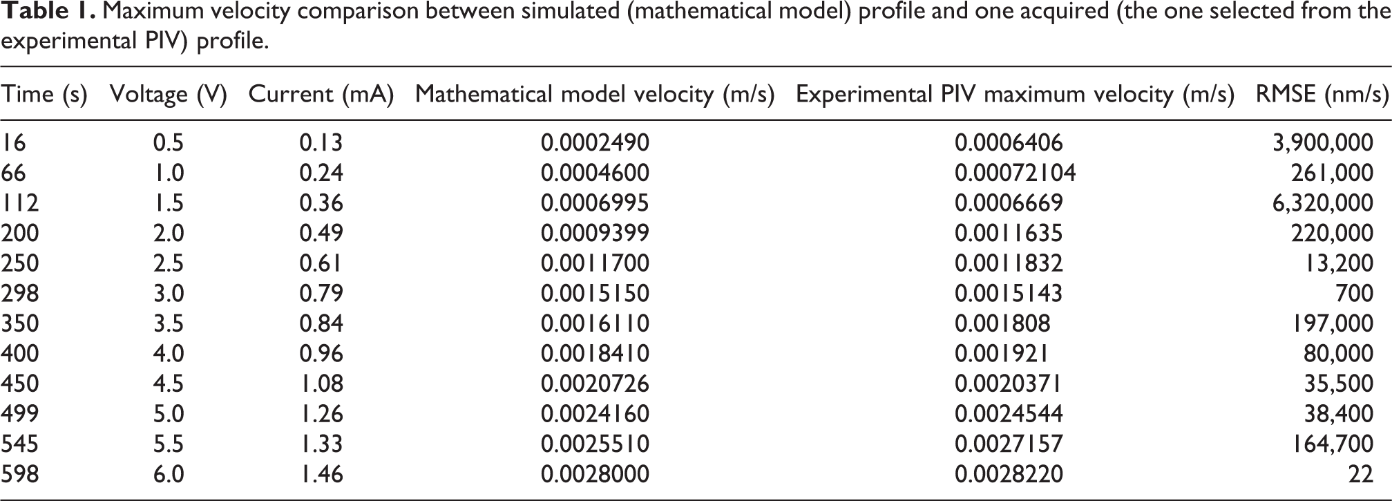
Maximum velocity comparison between simulated (mathematical model) profile and one acquired (the one selected from the experimental PIV) profile.

Time (s)	Voltage (V)	Current (mA)	Mathematical model velocity (m/s)	Experimental PIV maximum velocity (m/s)	RMSE (nm/s)
16	0.5	0.13	0.0002490	0.0006406	3,900,000
66	1.0	0.24	0.0004600	0.00072104	261,000
112	1.5	0.36	0.0006995	0.0006669	6,320,000
200	2.0	0.49	0.0009399	0.0011635	220,000
250	2.5	0.61	0.0011700	0.0011832	13,200
298	3.0	0.79	0.0015150	0.0015143	700
350	3.5	0.84	0.0016110	0.001808	197,000
400	4.0	0.96	0.0018410	0.001921	80,000
450	4.5	1.08	0.0020726	0.0020371	35,500
499	5.0	1.26	0.0024160	0.0024544	38,400
545	5.5	1.33	0.0025510	0.0027157	164,700
598	6.0	1.46	0.0028000	0.0028220	22

2-D velocity profile analysis and smoothing tool

Considering the relevance of MHD applications in microfluidics, nonintrusive experimental methods and analysis technique have been sought to MHD quantitative flow computation, for which it is common to use the open-source MATLAB tool “PIVlab” created by William Thielicke ⁴² under the MATLAB platform. This tool is a graphical user interface (GUI) that allows the PIV to perform flow analysis, through digital image processing that calculates the velocity distribution in a frame sequence, and it is also used to calculate multiple parameters of the flow pattern in a general way. However, this GUI does not have any specific tool for MHD flow analysis, for this reason, an application was added to PIVlab to generate specific results on two dimensions for MHD flow analysis. The application “2-D velocity profile analysis and smoothing tool” aims to analyze the velocity profiles of a flow acting under a magnetic and electric field by smoothing and detecting outliers, using filters and regression methods for corrections. The tool that is being integrated into PIVlab takes as input data, files generated through PIVLab from which it is possible to select some parameters such as the frame ranges to be analyzed, the smoothing filters and regression methods for outlier’s detection and the detection of intensity variation. Also, it is possible to select up to 10 files simultaneously with a range of up to 25 frames per file with a variable points sample to perform the analysis in parallel between the different generated graphics. The system has the capacity to store all results in work variables easily recoverable by the user. The programmed tool is part of the PIVlab options menu as an additional section as shown in Figure 4. This additional section can work independently as a tool for analysis and smoothing of 2-D velocity profiles of magnetohydrodynamic flow since it is possible to load the data files previously obtained from an image sequence processed by the PIVlab. This process can be observed in Figure 5. The data are extracted from text files containing two information fields corresponding to the distance measured from the center of the plotted area and the tangential velocity of the particles in that selected area. The data are filtered through different methods such as moving, lowess, loess, sgolay, rlowess, and rloess which are selected from the interface (type filter). The detection intensity variation is obtained by means of a scroll bar that low value of 0.01 in the left end, its increment is 0.01 to the right until reaching the 0.99 top values (filter value). This algorithm can be seen in Figure 6.

Figure 4.

(a) General view of the interface “2-D Flow Velocity MHD” as a tool added to PIVlab. (b) Original PIVlab settings options. (c) 2-D velocity profile analysis and smoothing tool added to PIVlab. MHD: magnetohydrodynamic; PIV: particle image velocimetry.

Figure 5.

Loading of data files generated by PIVlab. PIV: particle image velocimetry.

Figure 6.

Data filtering process.

Technique for 2-D velocity profile enhancement

From a big collection of videos for MHD 2-D velocity profile measurement, 1 s of video of experiment C described in Table 1 of publication ¹⁷ with induced fields B ₀ = 0–1624 T and ϕ = 5 V, I = 1.87 mA with a maximum velocity of 0.0035 m/s was extracted to apply PIV and create a 25 × 400 database, where each column corresponds to a camera shot each 40 ms and every row corresponds to the channel width position where the velocity was measured (400 measurements were performed through the whole channel width). The database has been submitted to eliminate outliers and for smooth processing to approximate measurements to the simulated model.

Data mining for outliers elimination

An outlier is an observation point that is distant from other observations. The cause of the presence of outliers in a database may be due to variability in the measurement or it may indicate experimental errors. There exist plenty of methods to identify and eliminate outliers; some are based on visualization, while others are based on mathematical procedures. ¹⁹ In this experimentation, the outlier’s detection was based on the robust Mahalanobis distances (RMD). The Mahanalobis distance $(D_{\text{M}})$ is a matrix containing the RMD of each profile in its diagonal and it is calculated using equation (2), which is based on the calculation of the covariance distance between data to estimate the similarity of each profile. If X is a matrix with 25 rows $\left(i=1, \dots , 25\right)$ , each row is a profile (a profile measurement every 40 ms), and 400 columns $\left(j=1, \dots , 400\right)$ , each column value of one row contains the velocity of the profile at the consecutive distances through the channel width, it is from position in distance 1 (internal cylinder) to distance to position 400 (external cylinder). The μ is a matrix of 25 rows with 400 columns with mean ${\mu }_j\hspace{0.17em}\left(j=1,\dots ,400\right)$ , which means each row of the μ matrix is equal, and each value in a column for all the rows corresponds to the mean of the corresponding column from the X matrix, see equations (3) and (4). The ${\sum }^{-1}$ is the inverse covariance matrix of the whole database X of 25 rows by 400 columns, see matrix in equation (5), where each row is an observation, and each column a variable. The $\sum$ covariance matrix of X for which the input is $\left(i,j\right)$ is the covariance calculated using equations (6) and (7), while the inverse covariance ${\sum }^{-1}$ of matrix X is calculated by processing the covariance matrix $\sum { }^{ }$ using equation (8). Finally, the $D_{\text{M}}$ matrix diagonal values from the 25 rows are compared with a threshold to determine if the profile is an outlier or not

$D_{\text{M}}\left(x_{ij}\right)=\sqrt{{\left(X-\mu \right)}^{\text{T}}{\sum }^{-1}\left(X-\mu \right)}$

2

$\text{for }i=1:25{\mu }_i=\frac{1}{400}{\displaystyle \sum }_{j=1}^{j=400}{x}_{ij}$

3

$\mu =\left[\begin{array}{ccc}{\mu }_1& \cdots & {\mu }_{25}\\ ⋮& \ddots & ⋮\\ {\mu }_1& \cdots & {\mu }_{25}\end{array}\right]$

4

$X=\left[\begin{array}{ccc}{x}_{11}& \cdots & x_{1,400}\\ ⋮& \ddots & ⋮\\ x_{25,1}& \cdots & x_{ij}\end{array}\right]=\left[\begin{array}{ccc}{x}_{1,1}& \cdots & x_{1,400}\\ ⋮& \ddots & ⋮\\ x_{25,1}& \cdots & x_{25,400}\end{array}\right]$

5

${\sum }_{ij=}E\left[\left(x_i-{\mu }_i\right)\left(x_i-{\mu }_j\right)\right]$

6

$\sum =\left[\begin{array}{cccc}E\left[\left(x_1-{\mu }_1\right)\left(x_1-{\mu }_1\right)\right]& E\left[\left(x_1-{\mu }_1\right)\left(x_2-{\mu }_2\right)\right]& \cdots & E\left[\left(x_1-{\mu }_1\right)\left(x_j-{\mu }_j\right)\right]\\ E\left[\left(x_2-{\mu }_2\right)\left(x_1-{\mu }_1\right)\right]& E\left[\left(x_2-{\mu }_2\right)\left(x_2-{\mu }_2\right)\right]& \cdots & E\left[\left(x_2-{\mu }_2\right)\left(x_j-{\mu }_j\right)\right]\\ ⋮& ⋮& \ddots & ⋮\\ E\left[\left(x_i-{\mu }_i\right)\left(x_1-{\mu }_1\right)\right]& E\left[\left(x_i-{\mu }_i\right)\left(x_2-{\mu }_2\right)\right]& \cdots & E\left[\left(x_i-{\mu }_i\right)\left(x_j-{\mu }_j\right)\right]\end{array}\right]$

7

${\sum }^{-1}=\frac{1}{\text{det}\left(\sum \right)}{\left[\sum \right]}^{\text{T}}$

8

From the 25 original profiles, 4 of them were considered outliers and were eliminated (profiles from frames # 2, 8, 12, and 18). Obtaining a 21 × 400 new database, results are shown in Figure 7 where the green dash-dot line corresponds to the 2-D velocity model simulation, and the other 21 lines correspond to the 2-D velocity measurement of each camera frame not considered outlier.

Figure 7.

2-D velocity profile comparison of simulation and measurement results (without outliers).

Filtering for smoothing

The filtering process is a kind of signal processing to remove unwanted features from a signal. For this application, the purpose of filtering the 2-D velocity profiles is to smoothing the profiles to reduce and/or eliminate the roughness (positive and negative peaks in the profiles) to create an approximation to the 2-D velocity profile simulated by the MHD stirrer governing mathematical model. The MATLAB smooth function has been selected to perform the profiles smoothing. The methods available were evaluated:

Moving average filtering (moving). It smoothens data by replacing each data point with the average of the neighboring data points defined within a span.

Savitzky–Golay filtering (sgolay). A generalized moving average also called a digital smoothing polynomial filter or a least squares smoothing filter.

Local regression smoothing. It uses local regression using weighted linear least squares and a first-degree polynomial model (lowess), and a robust version of “lowess” that assigns lower weight to outliers in the regression. The method assigns zero weight to data outside six mean absolute deviations (rlowess). It uses local regression using weighted linear least squares and a second-degree polynomial model (loess), and a robust version of “loess” that assigns lower weight to outliers in the regression. The method assigns zero weight to data outside six mean absolute deviations (rloess).

Profile from frame #1 was used to evaluate all the filtering methods within the span values [0.01:0.01:0.99], and it was found that the best results were provided by methods “sgolay” and “rloess” computed with span value 0.79. Filtering methods and parameters evaluation is shown in Figure 8; in each image ((a) to (d)), the green dash-dot line corresponds to the 2-D velocity model simulation, the red dash-dot line corresponds to the profile from frame #1, and the rest of the lines correspond to the smoothing profiles from the corresponding filter for each span values 0.01, 0.02, 0.03,…, 0.99.

Figure 8.

Filtering methods and parameters evaluation: (a) moving average filtering, (b) Savitzky–Golay filtering, (c) robust version of local regression using weighted linear least squares and a first-degree polynomial model, and (d) robust version of local regression using weighted linear least squares and a second-degree polynomial model.

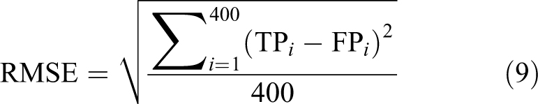
Once the method (rloess) and the span value were selected (0.79), it was applied to the 21 × 400 new database (without outlier’s). The 21 2-D velocity profiles smoothed were averaged as shown in Figure 9(a), where it is observed that the averaged profile (blue dash-dot line) lost velocity amplitude in comparison with the 21 profiles smoothed due to the filtering (the rest of the lines with except of green dash-dot that corresponds to the 2-D velocity model simulation). As a correction, a proportionality constant k was evaluated with values [1.00:0.05:2.00], obtaining the best results with k = 1.35. Concluding the data processing, Figure 9(b) shows the final 2-D velocity profile (blue dash-dot line) in comparison with the 2-D velocity model simulation (green dash-dot line). The difference between target profile (TP) and the final profile (FP) obtained was evaluated through root-mean-square error (RMSE) using equation (9), obtaining a successful velocity RMSE value of 207 nm/s

$\text{RMSE}=\sqrt{\frac{{{\displaystyle \sum }}_{i=1}^{400}{\left({\text{TP}}_i-{\text{FP}}_i\right)}^2}{400}}$

9

Figure 9.

Filtering results: (a) filtering results of 21 × 400 database (without outlier’s) and (b) 2-D velocity profile measurement after data processing (blue dash-dot line) in comparison with the 2-D velocity model simulation (green dash-dot line).

Experimentation methodology and results

After the technique for 2-D velocity profile enhancement has been defined and ran through a standard experiment taken from the study by Valenzuela-Delgado et al., ¹⁷ new experimentation has been designed and performed to validate the output performance of the proposed technique.

One hundred milliliters of distilled water was seeded with 0.1 g of S-HGS particles to fill the MHD stirrer, the electrodes were connected to a power supply and power on at the same time that the camera recorder with 0.5 V increments every velocity profile measurement (approximately every 50 seconds), obtaining results shown in Figure 10. A video with 11:45.36 (17,509 frames) was recorded, which is presented in 12 images (every minute) to show the MHD stirrer behavior, see Figure 11.

Figure 10.

Green dash-dote lines correspond to the simulated profiles at every voltage value at a specific time (according to Table 1). The rest of the lines corresponds to the 300 velocity profiles (25 at every voltage value).

Figure 11.

MHD stirrer behavior (flow mixing). MHD: magnetohydrodynamic.

2-D velocity profile’s maximum velocity value measurement

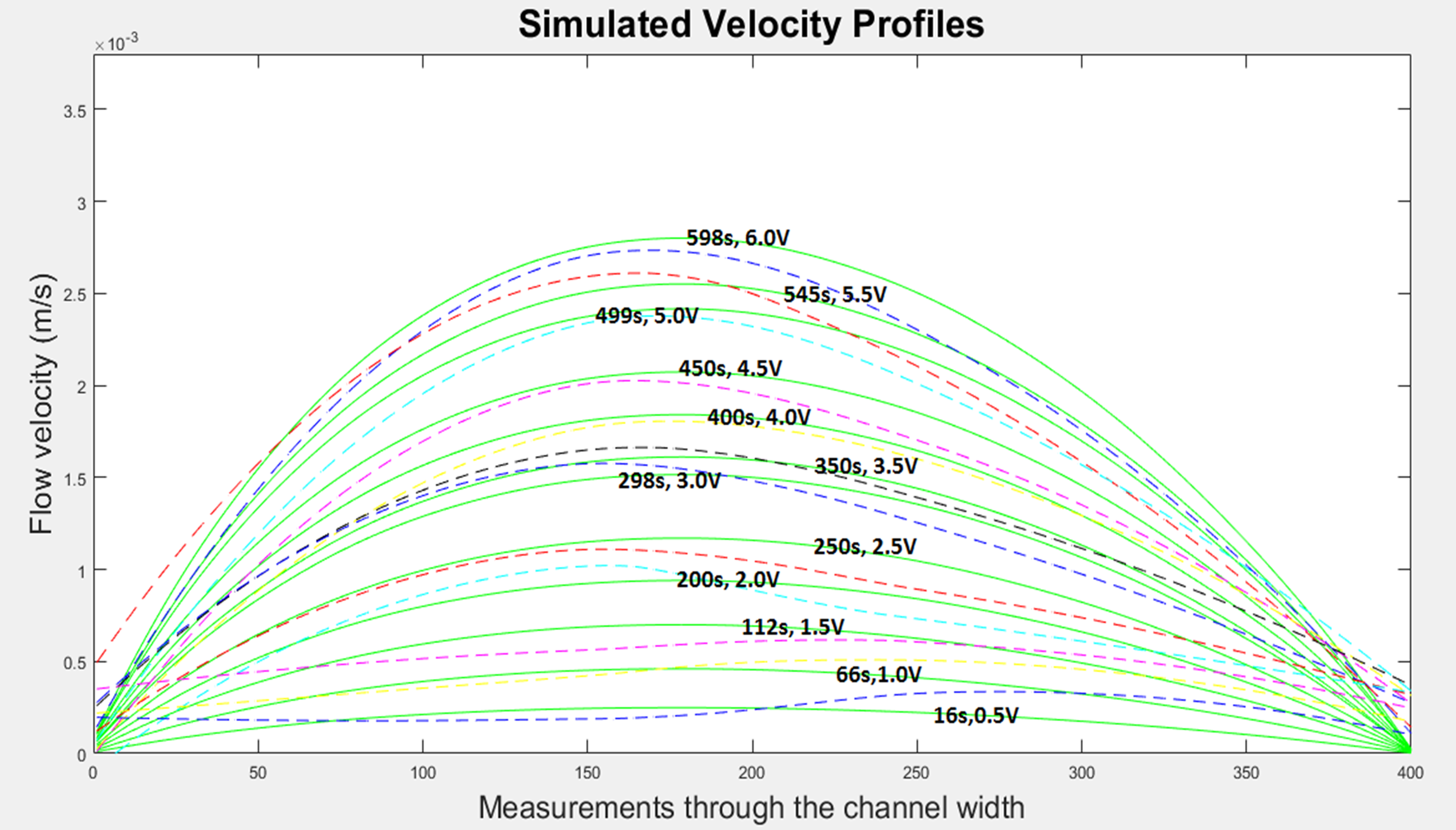
The first evaluation consists of the measurement of the maximum velocity found in the 2-D velocity profile. Twelve 2-D velocity profiles were selected. In every 0.5 V increments, 25 2-D velocity profiles were acquired in every voltage increment (0.5:0.5:6.0 V), of each batch, the profile with the maximum velocity more close to the maximum velocity simulated was selected and compared through the RMSE as shown in Figure 12 and Table 1.

Figure 12.

Green lines correspond to the simulated profiles at every voltage value at a specific time (according to Table 1). The rest of the lines corresponds to the selected velocity profile for each voltage value.

Complete 2-D velocity profile measurement

As proposed in the “Technique for 2-D velocity profile enhancement” section, the technique for 2-D velocity profile enhancement was applied to each of the velocity profile batch (25 velocity profiles) of every 0.5 V increments. Firstly, the complete 2-D velocity profiles of the selected profiles used on the evaluation of the “2D Velocity Profile’s Maximum Velocity Value Measurement” section were compared with the simulated profiles through the RMSE as shown in Table 2. Secondly, the outliers were removed from each batch of profiles, then the remaining 2-D velocity profiles in each batch were filtered with “rloess” computed with span value 0.79, smoothed profiles from each batch were averaged and compensated with a proportionality constant k, and finally compared with the simulated profiles, as presented in Table 2 and visually compared in Figure 13 and detailed in Figure 14.

Table 2.

Complete velocity profile comparison: (a) selected 2-D velocity profile versus simulated profile and (b) 25 2-D velocity profile after data processing versus simulated profile.

Voltage (V)	Current (mA)	Time (s)	Selected 2-D velocity profile versus simulated profile		25 2-D velocity profile after data processing versus simulated profile
			Frame Range #	RMSE(nm/s)	Frame Range#	k	RMSE(nm/s)
0.5	0.13	16	402–403	51.825	550–575	0.57	10.096
1.0	0.24	66	1659–1660	33.027	1650–1675	0.85	10.380
1.5	0.36	112	2821–2822	94.177	2800–2825	1.10	13.576
2.0	0.49	200	5011–5012	88.344	5000–5025	1.40	10.151
2.5	0.61	250	6264–6265	106.710	6250–6275	1.00	10.455
3.0	0.79	298	7458–7459	209.690	7450–7475	1.10	11.688
3.5	0.84	350	8772–8773	126.340	8750–8775	0.93	10.716
4.0	0.96	400	10,024–10,025	135.370	10,000–10,025	0.93	10.033
4.5	1.08	450	11,268–11,269	139.880	11,250–11,275	0.89	11.033
5.0	1.26	499	12,489–12,490	158.690	12,475–12,500	0.97	13.634
5.5	1.33	545	13,627–13,628	66.243	13,625–13,650	0.95	23.670
6.0	1.46	598	14,974–14,975	59.400	14,950–14,975	0.93	16.763

PIV: particle image velocimetry.

Figure 13.

Green lines correspond to the simulated profiles at every voltage value at a specific time (according to Table 1). The rest of the lines corresponds to the processed velocity profile batch for each voltage value.

Figure 14.

Purple lines are velocity profiles remaining after outlier elimination for every value at a specific time (according to Table 1). Green lines correspond to the simulated profiles at every voltage value at a specific time. Dark blue lines correspond to the selected velocity profiles shown in Figure 12 and evaluated in Table 1. Light blue lines correspond to the processed resulting profiles to feedback to the measurement system, also shown in Figure 13 and evaluated in Table 2.

Conclusion

For the development of MEMS based on MHD for micro-robot applications which require precise control of micro-flow behavior, a technique was developed for the enhancement of a PIV measurement process in a customized machine vision system. The PIV measurements were performed for the micro-flow complete 2-D velocity profile mathematical model validation of an MHD stirrer prototype. Data mining and filtering have been applied to a raw measurement database from the customized machine vision system designed to evaluate the MHD stirrer prototype. Outlier’s elimination and smoothing have been applied to raw data to approximate the PIV measurements output to the complete 2-D velocity profile mathematical model to increase the accuracy of a customized machine vision system for complete 2-D velocity profile measurements. In comparison with previous research in the state of the art that only compare the maximum velocity ^44,45 ; with the proposed technique, the complete 2-D velocity profiles can be evaluated. The “2D Velocity Profile’s Maximum Velocity Value Measurement” section has explained how to perform the traditional measurement of the maximum velocity, which is necessary to look for the profile with the minimum RMSE_{(max. velocity)} in a batch of profiles. Table 1 presents how the maximum velocities RMSE vary in the range of 22–6,320,000 nm/s. While in Table 2, the same velocity profile is detailed as how the complete velocity profiles RMSE vary in the range of 33–209 nm/s. Finally, Table 2 also presents how after applying the proposed technique the complete velocity profiles RMSE vary in the range of 10–23 nm/s. With the enhancement achieved, the measurement system is ready to proceed to the construction of the 3-D velocity profile of the MHD stirrer prototype. The presented methodology can be used for measurement and validation in the design of MEMS micro-robots and of any devices that require micro-flow manipulation for tasks such as stirring, pumping, mixing, networking, propelling, and even cooling.