Sage Journals: Discover world-class research

Abstract

This article presents a geometric approach for path planning of serpentine manipulator for real-time control in confined spaces. Firstly, the mechanical design of a serpentine manipulator is introduced, and its kinematics is analyzed. As the serpentine manipulator usually has more than 10 degrees of freedom, the motion control and obstacle avoidance are difficult considering its inverse kinematics. Follow-the-leader is an ideal path planning method for serpentine manipulator, as the manipulator moves forward, all the sections follow the path that the tip of manipulator has passed, which simplifies the obstacle avoidance. The realization of follow-the-leader method is to find the new configurations of the manipulator that can fit the ideal path with small errors. In this article, a novel geometric approach for follow-the-leader motion is proposed to solve new configurations with high precision of location and less computation time. The method is validated through simulation and the deviation from the ideal path is analyzed, simulation results show that calculation time for per step is less than 0.5 ms for a serpentine manipulator with 10 sections. To verify the follow-the-leader method, a 13-degree-of-freedom serpentine manipulator system with 6 sections was built, and 12 magnetic rotary encoders were embedded into the universal joints to collect data of rotation angles of each section. Experimental results show that the manipulator can carry out follow-the-leader motion as expected in real time.

Keywords

Serpentine manipulator follow-the-leader geometric approach kinematics hyper-redundant

Introduction

To solve the problem that the traditional robot is difficult to carry out high-efficiency operation in confined space, serpentine manipulator is developed. The introduction of redundant sections enables the serpentine manipulator to achieve desired tip position more flexibly, thus it is also called hyper-redundant manipulator. The serpentine manipulator has a strong obstacle avoidance capability, making it particularly suitable for use as a special robot, which can enter the enclosed space through small holes or cracks, then carries out operations, laser cutting or repair work.

In this field, since the term hyper-redundant was coined by Chirikjian and Burdick in 1991,¹ many designs of serpentine manipulator system have been put forward by different research teams. They can be divided into two categories, rigid structure serpentine manipulator and continuum manipulator. Walker and Colleagues^2
–4 developed a cable-driven manipulator and the kinematic modeling was carried out. Rigid structure serpentine manipulator developed by the OC robotics,^5,6 a company in United Kingdom, has been used in the assembly of commercial aircraft. The concept of continuum manipulator was put forward by Robinson and Davies in 1999,⁷ which is usually formed by flexible materials such as spring and elastic rod. Festo pneumatic components company⁸ in Germany launched a flexible pneumatic continuum manipulator, the flexibility of the gripper arm allows direct human–machine contact, and a large number of commonly used medical devices such as catheters and colonoscopes can be considered continuum manipulator.⁹

But because of some restrictions on their own, these manipulators have certain limitations, the load capacity of continuum manipulator is relatively low because of its flexible material characteristics, and its end positioning accuracy is poor. The medical endoscopes only have one to two controllable joints; they lack the ability to fully explore the complex structure of the deep cavity, and it is impossible for them to achieve the work of high payload. In this article, we design a rigid-backbone serpentine manipulator, in which each section can be controlled independently, to achieve better load capacity and positioning accuracy.

As the serpentine manipulator relies on its redundancy, the obstacle avoidance is very important for it. Many path planning methods have already been proposed. Asano¹⁰ proposed a motion planning method based on the sequential method. A planar obstacle avoidance algorithm termed “tunneling” was proposed by Chirikjian and Burdick.¹ Conkur¹¹ proposed a path following algorithm using B-spline curves, and the sections of a hyper-redundant manipulator are required to remain approximately tangent to the curves. Bozek and Pokorny¹² proposed a new method of calculating Jordan curves trajectory based on the intrinsic properties of the plane. A predetermined environment is a necessary condition for most path planning algorithms, but the environmental data cannot be easily obtained in an emergency or some unknown environment. Although environmental modeling can be carried out by sensors,¹³ the position of obstacle may change by time in some dangerous sites, such as the cutter head in work chamber of shield machine. The sensors will greatly increase the complexity of the system.

Another approach for path planning of the serpentine manipulator is follow-the-leader. When the manipulator advances toward a desired position, the tip of distal section guides the direction of the manipulator, then a new arrangement to the new position is calculated which minimizes the deviation from the path already traveled. Follow-the-leader method is particularly suitable for the manual control of the manipulator when combined with machine vision. With a camera embedded in the end-effector, the user can easily navigate the manipulator through controlling the direction of the distal section according to the image of obstacle from the camera, while advancing the base of it.

Follow-the-leader method was adapted to payload inspection and processing system in 1994.^14,15 Neumann and Burgner-Kahrs¹⁶ proposed a method to generate follow-the-leader motion of tendon-driven continuum robots with extensible sections for general paths in three-dimensional (3-D). Palmer et al.¹⁷ proposed a tip following method using the sequential quadratic programming optimization approach to navigate the continuum manipulator. A follow-the-leader control for a binary actuated hyper-redundant manipulator was proposed by Tappe et al.,¹⁸ which only works for the manipulator with a serial chain of continuous actuators. Aristidou et al.¹⁹ proposed a FABRIK algorithm for inverse kinematics of human joints. The algorithm has low computational cost and produces visually realistic poses. The new position of joint in FABRIK method is on the line between the current position and the target position of the next joint, so there is a certain distance between the joint and the manipulator, and the displacement of the overall configuration of the manipulator is relatively large.

Follow-the-leader algorithms are usually realized by numerical method, as new arrangement should be found with a certain tolerance, which becomes a constrained optimization problem. However, the computation time becomes the main constraint for the control performance of the manipulator. When implementing follow-the-leader method to continuum manipulator, there is an oscillating error in the tip position,¹⁷ which may cause problem to the images from the camera when operated in manual mode.

The main contribution of this article is to propose a novel follow-the-leader method for rigid-backbone serpentine manipulator with high precision of location and less computation time. This method is suitable for following a predefined 3-D path and manual navigation under machine vision, as each joint will be on the path and there is no deviation in tip position theoretically. To calculate the new arrangements of follow-the-leader motion, a geometric approach is proposed, and the analytic solution for the inverse kinematics of configuration space to task space mappings is obtained under the condition that the position of each joint is known. Thus, solving new arrangements by numerical method is avoided and there are no any nonlinear equations to solve, which greatly reduces the calculation time to achieve real-time control.

The remainder of this article is structured as follows: firstly, the mechanical design of a cable-driven serpentine manipulator is introduced. In the following section, the kinematics of serpentine manipulator is analyzed. Then, geometric approach for follow-the-leader is introduced in detail and the algorithm to follow a predefined path is presented subsequently. In the next section, simulation results are presented and the performance of follow-the-leader motion is analyzed. Finally, experimental validation for the follow-the-leader method is carried out on the hardware.

Mechanical design of the serpentine manipulator

The schematic of the whole system is shown in Figure 1 The serpentine manipulator system consists of actuation module, manipulator module, and feed-in module. The manipulator module has six sections, each section has two degrees of freedom (DOFs). The distal section is equipped with a camera, a gripper, and a laser. The actuation module is set in a pack at the base of the manipulator, which consists of transmission mechanisms and motors. The base of the manipulator is mounted on a horizontal sliding table, while the horizontal sliding table is fixed on a lifting platform, they are the feed-in module, which make the whole manipulator have a horizontal linear DOF and a vertical linear DOF. The horizontal sliding table is a ball screw slide driven by servomotor, while the lifting platform is equipped with two hydraulic cylinders driven by proportional valves.

Figure 1.

Schematic of the whole manipulator system.

Manipulator module design

Manipulator module has six sections connected in series. Each section consists of two end disks and a hollow cylinder, which are made of aluminum alloy to reduce weight. As shown in Figure 2, every two sections are connected by a special universal joint. This special hollow universal joint has two vertical shafts, therefore each section has two rotational DOF. Each section and joint have central holes in which electrical wires can go through. As cable can only transfer pulling force, one section should be driven by at least three cables. In this design, each section is driven by three steel wire ropes evenly spaced along the circumference (120° apart). The positions of cables driving each section are separated from each other with fixed angle, therefore the driving cables will go through the hole in end disk of the former sections and eventually connected to the driving module. Friction will inevitably occur between driving cable and the hole in the end disk, in that case, the wear of the hole may lead to a reduction in precision. Thus, a sleeve with heat treatment is mounted in each hole that the driving cable passes through. As the sleeves are harder than the driving cables, only the driving cables will be worn, and it is more convenient to replace the driving cables rather than the sleeves.

Figure 2.

Illustration of the manipulator module.

Actuation system design

Driving module consists of driving components, as shown in Figure 3. The function of driving module is to transfer the power of motors to the driving cables. Each diving component consists of a coupling, a bearing seat, a ball screw pair, an Linear Motion (LM) shaft, and a connection board. As the driving cables are distributed on the circle of end disk, the motors should distribute on a larger circle as the diameter of motor is larger than that of the driving cable. A connection board is used to connect driving cable and the ball screw pair, and an LM shaft is also needed to make the diving component have a single, linear DOF. The ball screw pair setting on the bearing seat is connected to servomotor through a coupling. The bearing seats and LM shaft are mounted on the supporting board. Thus, the displacement of the driving cable can be controlled by the rotation of the servomotor.

Figure 3.

Rendering diagram of driving module.

Kinematic modeling

The motion control of the manipulator is based on the kinematics model. In this field, Walker and Colleagues^20,21 proposed constant curvature model using curvature and angle of curvature to describe the shape of continuum robots. Chirikjian and Burdick²² used parameterized backbone curves based on amplitude varying and traveling wave gaits to analyze the kinematics of serpentine manipulator. As rigid-backbone serpentine manipulator has rigid links, these kinematics models are not suitable for its motion control. Due to the mechanic design of serpentine manipulator which has two DOFs for each section, the position and orientation of the manipulator can be described by the two rotation angles of each section. These rotation angles can be controlled by changing the lengths of the driving cables. Therefore, two mappings and three spaces define the kinematics of serpentine manipulator, as shown in Figure 4. The lengths of driving cables are defined as actuator space. The rotation angles of each section are defined as configuration space. While the position and orientation of the distal section is defined as task space. The kinematics is analyzed in this section, and the relationship between joint parameters, actuation parameters, and joints positions is given.

Figure 4.

The three spaces and mappings between them which define the kinematics of serpentine manipulator.

Configuration space to task space kinematics analysis

The kinematics analysis from configuration space to task space illustrates the relationship between the rotation angles of each section and position and orientation of the distal section. The kinematics model based on geometric relation is established as shown in Figure 5, and each joint has a coordinate frame attached to it, the origin of the coordinate frame is the center of the universal joint, the axis of the joint is Y-axis, the vertical axis is the Z-axis, and the X-axis is determined by the right-hand system. Ψ _n = {X_n , Y_n , Z_n } is the coordinate frames of joint n. 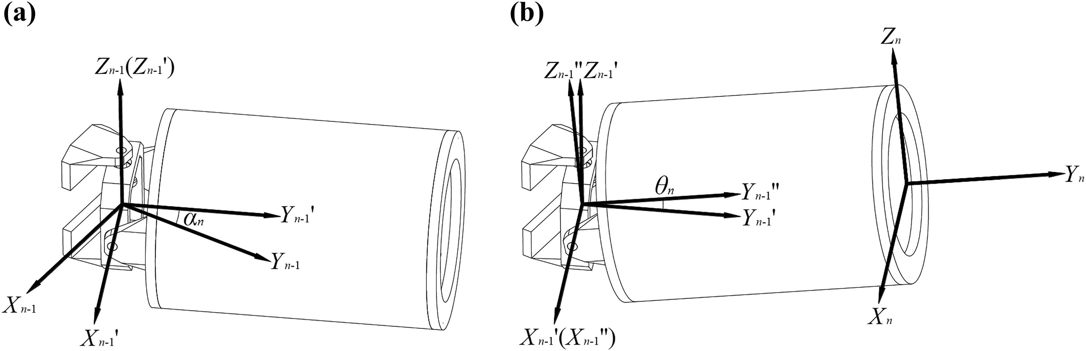While $Ψ_{n - 1}^{'}$ and $Ψ_{n - 1}^{″}$ are the transition coordinate frames between Ψ _n− ₁ and Ψ _n . As each section has two DOFs, two rotation angles are introduced, pitch angle θ is defined as the rotation angle of the horizontal axis of the universal joint and yaw angle α is the rotation angle of the vertical axis of the joint. The distance between the centers of every two joints is L.

Figure 5.

Representation of single section with joint parameters and coordinate frames: (a) local coordinate system of joint n rotates αn degree around its Z-axis (b) then it rotates θn degree around its X axis and translates L distance along Y axis to the local coordinate system of joint n-1.

The transformation from Ψ _n ₋₁ to Ψ _n can be carried out using homogeneous coordinate transformation in equation (1), and ^BR_E represents the transformations matrix. Matrix [n o a] is the projection of unit vectors on the XYZ axis of the terminal coordinates in the base coordinates, while matrix [p] is the position vector of the terminal coordinates to the base coordinates

{}^{B}R ​_{E} = [\begin{matrix} n & o & a & p \\ 0 & 0 & 0 & 0 \end{matrix}] = [\begin{matrix} n_{x} & o_{x} & a_{x} & p_{x} \\ n_{y} & o_{y} & a_{y} & p_{y} \\ n_{z} & o_{z} & a_{z} & p_{z} \\ 0 & 0 & 0 & 1 \end{matrix}]

Due to the geometric model, one realization of the transformation ⁿ ⁻¹ R_n is as follows: (1) Ψ _n ₋₁ rotate α_n degree around its Z-axis to $Ψ_{n - 1}^{'}$ , (2) rotate θ_n degree around its X-axis to $Ψ_{n - 1}^{″}$ , and (3) translate L distance along Y-axis to Ψ _n . The above transformations are all based on the self-coordinate system. Thus, the transformation matrix between Ψ _n ₋₁ and Ψ _n is shown in equation (2)

\begin{matrix} {}^{n - 1}R ​_{n} = Rot (z, α_{n}) \cdot Rot (x, θ_{n}) \cdot Trans (L) \\ = [\begin{matrix} c_{α_{n}} & - s_{α_{n}} & 0 & 0 \\ s_{α_{n}} & c_{α_{n}} & 0 & 0 \\ 0 & 0 & 1 & 0 \\ 0 & 0 & 0 & 1 \end{matrix}] \cdot [\begin{matrix} 1 & 0 & 0 & 0 \\ 0 & c_{θ_{n}} & - s_{θ_{n}} & 0 \\ 0 & s_{θ_{n}} & c_{θ_{n}} & 1 \\ 0 & 0 & 0 & 1 \end{matrix}] \cdot [\begin{matrix} 1 & 0 & 0 & 0 \\ 0 & 1 & 0 & L \\ 0 & 0 & 1 & 0 \\ 0 & 0 & 0 & 1 \end{matrix}] \end{matrix}

As a result, the forward kinematics from the joint space to task space can be written as equation (3). ⁰ R_n can be used to describe the position and pose of section n relative to the base coordinates

{}^{0}R_{n} = {}^{0}R ​_{1} \cdot {}^{1}R ​_{2} \cdot \dots \cdot {}^{n - 2}R ​_{n - 1} \cdot {}^{n - 1}R ​_{n}

Joints positions to configuration space kinematics analysis

For the hyper-redundancy of serpentine manipulator, there is no analytic solution for the inverse kinematics of configuration space to task space mappings. However, if positions of all the joints are known, the rotation angles of each section can be calculated. It is useful for the follow-the-leader method proposed in this article. Therefore, only joints positions to configuration space kinematics analysis are discussed in this section.

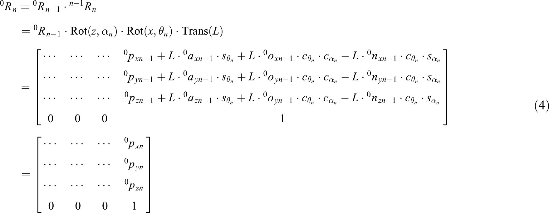
Assuming that the position of section n and the pose matrix of section n − 1 are known. From equations (2) and (3), when n > 1 the pose matrix of section can be expressed as equation (4), only the position vector of the pose matrix is needed here, so other items of the matrix are omitted

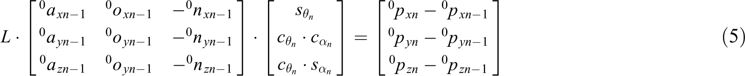
\begin{array}{l} {}^{0}R ​_{n} = {}^{0}R ​_{n - 1} \cdot {}^{n - 1}R ​_{n} \\ = {}^{0}R ​_{n - 1} \cdot Rot (z, α_{n}) \cdot Rot (x, θ_{n}) \cdot Trans (L) \\ = [\begin{matrix} \dots & \dots & \dots & {}^{0}p ​_{x n - 1} + L \cdot {}^{0}a ​_{x n - 1} \cdot s_{θ_{n}} + L \cdot {}^{0}o ​_{x n - 1} \cdot c_{θ_{n}} \cdot c_{α_{n}} - L \cdot {}^{0}n ​_{x n - 1} \cdot c_{θ_{n}} \cdot s_{α_{n}} \\ \dots & \dots & \dots & {}^{0}p ​_{y n - 1} + L \cdot {}^{0}a ​_{y n - 1} \cdot s_{θ_{n}} + L \cdot {}^{0}o ​_{y n - 1} \cdot c_{θ_{n}} \cdot c_{α_{n}} - L \cdot {}^{0}n ​_{y n - 1} \cdot c_{θ_{n}} \cdot s_{α_{n}} \\ \dots & \dots & \dots & {}^{0}p ​_{z n - 1} + L \cdot {}^{0}a ​_{z n - 1} \cdot s_{θ_{n}} + L \cdot {}^{0}o ​_{y n - 1} \cdot c_{θ_{n}} \cdot c_{α_{n}} - L \cdot {}^{0}n ​_{z n - 1} \cdot c_{θ_{n}} \cdot s_{α_{n}} \\ 0 & 0 & 0 & 1 \end{matrix}] \\ = [\begin{matrix} \dots & \dots & \dots & {}^{0}p ​_{x n} \\ \dots & \dots & \dots & {}^{0}p ​_{y n} \\ \dots & \dots & \dots & {}^{0}p ​_{z n} \\ 0 & 0 & 0 & 1 \end{matrix}] \end{array}

Reorganizing equation (4), one can obtain equation (5), it is a three element first-order equation

L \cdot [\begin{matrix} {}^{0}a ​_{x n - 1} & {}^{0}o ​_{x n - 1} & - {}^{0}n ​_{x n - 1} \\ {}^{0}a ​_{y n - 1} & {}^{0}o ​_{y n - 1} & - {}^{0}n ​_{y n - 1} \\ {}^{0}a ​_{z n - 1} & {}^{0}o ​_{y n - 1} & - {}^{0}n ​_{z n - 1} \end{matrix}] \cdot [\begin{matrix} s_{θ_{n}} \\ c_{θ_{n}} \cdot c_{α_{n}} \\ c_{θ_{n}} \cdot s_{α_{n}} \end{matrix}] = [\begin{matrix} {}^{0}p ​_{x n} - {}^{0}p ​_{x n - 1} \\ {}^{0}p ​_{y n} - {}^{0}p ​_{y n - 1} \\ {}^{0}p ​_{z n} - {}^{0}p ​_{z n - 1} \end{matrix}]

After solving equation (5), sin(θ_n ) and cos(θ_n ) · sin(α _n) can be acquired as equation (6), and two rotation angles can be calculated as equation (7)

[\begin{matrix} s_{θ_{n}} \\ c_{θ_{n}} \cdot c_{α_{n}} \\ c_{θ_{n}} \cdot s_{α_{n}} \end{matrix}] = L^{- 1} \cdot {[\begin{matrix} {}^{0}a ​_{x n - 1} & {}^{0}o ​_{x n - 1} & - {}^{0}n ​_{x n - 1} \\ {}^{0}a ​_{y n - 1} & {}^{0}o ​_{y n - 1} & - {}^{0}n ​_{y n - 1} \\ {}^{0}a ​_{z n - 1} & {}^{0}o ​_{y n - 1} & - {}^{0}n ​_{z n - 1} \end{matrix}]}^{- 1} \cdot [\begin{matrix} {}^{0}p ​_{x n} - {}^{0}p ​_{x n - 1} \\ {}^{0}p ​_{y n} - {}^{0}p ​_{y n - 1} \\ {}^{0}p ​_{z n} - {}^{0}p ​_{z n - 1} \end{matrix}]

\begin{array}{l} θ_{n} = arcsin (s_{θ_{n}}) \\ α_{n} = arcsin (s_{α_{n}}) \end{array}

When n = 1, the two rotation angles can be acquired as equation (8)

\begin{array}{l} θ_{1} = arcsin \frac{{}^{0}p ​_{z 1}}{\sqrt{{}^{0}p_{​_{y 1}}^{2} + {}^{0}p_{​_{z 1}}^{2}}} \\ α_{1} = arcsin \frac{- {}^{0}p ​_{x 1}}{\sqrt{{}^{0}p_{​_{y 1}}^{2} + {}^{0}p_{​_{z 1}}^{2}}} \end{array}

After that, θ ₁ and α ₁ can be acquired using equation (8), then ⁰ R ₁ can be calculated using equation (2), and θ ₂ and α ₂ can be acquire using equations (6) and (7). Thus, if position of all the joints is known, the rotation angles of each section θ ₁ and α ₁ can be calculated through the same process using equations (2), (6), (7), and (8).

Configuration space to actuator space kinematics analysis

The kinematics analysis from actuator space to configuration space is to calculate the displacement of each driving cable when the rotation angles are given.

Figure 6 provides a view of single-section module. It has three driving cables and two DOFs, so the single-section module is a parallel mechanism. It is easily known that the lengths of the cables in the section link will not change, according to its mechanic structure, only the lengths of cables between the distal disc in one section and its proximal disk in the next section will change the rotation angles. As a result, a simplified single-section model is established to calculate the relationship between lengths of driving cables and the rotation angles within a single section.

Figure 6.

Geometric illustration for solving cable length.

As shown by the geometry in Figure 6, the surface ABC and A ₁ B ₁ C ₁ represent distal disk in one section and proximal disk in the next section, which can be called disc 1 and disc 2, respectively. The line segments A ₁ B ₁, A ₂ B ₂, and A ₃ B ₃ represent three independent cables, l ₁, l ₂, and l ₃, respectively. Ψ₁= {X ₁, Y ₁, Z ₁} and Ψ₂= {X₂ , Y ₂, Z ₂} are attached to disc 1 and disc 2, respectively. Coordinate frames Ψ₁ and Ψ₂ have the same origins at point O, and it is also the center of the joint between these two sections. Y-axis of the coordinate frame is attached to the central axis of the section, the vertical axis is the Z-axis, and the X-axis is determined by the right-hand system.

Due to the geometric model, Ψ₁ rotates α degree around its Z-axis, then rotates θ degree around its X-axis, then it will coincide with Ψ₂. Thus, the transformation matrix between Ψ₁ and Ψ₂ is represented by equation (9)

\begin{matrix} {}^{1}R_{2} = Rot (z, α_{n}) \cdot Rot (x, θ_{n}) \\ = [\begin{matrix} c_{α} & - s_{α} & 0 & 0 \\ s_{α} & c_{α} & 0 & 0 \\ 0 & 0 & 1 & 0 \\ 0 & 0 & 0 & 1 \end{matrix}] \cdot [\begin{matrix} 1 & 0 & 0 & 0 \\ 0 & c_{θ} & - s_{θ} & 0 \\ 0 & s_{θ} & c_{θ} & 1 \\ 0 & 0 & 0 & 1 \end{matrix}] \end{matrix}

Taking a point A₁ on disk 1, as shown in Figure 6, $∠ A O' X' = β$ , one driving cable goes through A ₁ and B ₁ on disk 2, in the same way, $∠ B O' X' = β$ . ¹ A ₁ represents point A ₁ in Ψ₁

{}^{1}A ​_{1} = [\begin{matrix} - r \cdot sin β \\ - h \\ r \cdot cos β \end{matrix}]

In Ψ₂

{}^{2}B ​_{1} = [\begin{matrix} - r \cdot sin β \\ h \\ r \cdot cos β \end{matrix}]

Using the transformation matrix, B ₁ in Ψ₁ can easily be obtained in equation (10)

\begin{matrix} {}^{1}B ​_{1} = Rot (z, α_{n}) \cdot Rot (x, θ_{n}) \cdot {}^{2}B ​_{1} \\ = [\begin{matrix} r \cdot c_{β} \cdot s_{θ} \cdot s_{α} - h \cdot c_{θ} \cdot s_{α} - r \cdot s_{β} \cdot c_{α} \\ - r \cdot c_{β} \cdot s_{θ} \cdot c_{α} + h \cdot c_{θ} \cdot c_{α} - r \cdot s_{β} \cdot s_{α} \\ r \cdot c_{β} \cdot c_{θ} + h \cdot s_{θ} \end{matrix}] \end{matrix}

Then the length of cables A ₁ B ₁ can be determined in equation (11)

| {}^{1}A ​_{1} {}^{1}B ​_{1} | = | \begin{matrix} r \cdot c_{β} \cdot s_{θ} \cdot s_{α} - h \cdot c_{θ} \cdot s_{α} - r \cdot s_{β} \cdot (c_{α} - 1) \\ - r \cdot c_{β} \cdot s_{θ} \cdot c_{α} + h \cdot c_{θ} \cdot c_{α} + h - r \cdot s_{β} \cdot s_{α} \\ r \cdot c_{β} \cdot (c_{θ} - 1) + h \cdot s_{θ} \end{matrix} |

Calculating the value of determinant, equation (12) can be obtained as

\begin{matrix} | {}^{1}A ​_{1} {}^{1}B ​_{1} | = ({(r \cdot c_{β} \cdot s_{θ} \cdot s_{α} - h \cdot c_{θ} \cdot s_{α} - r \cdot s_{β} \cdot (c_{α} - 1))}^{2} + {(r \cdot c_{β} \cdot (c_{θ} - 1) + h \cdot s_{θ})}^{2} \\ + {{(- r \cdot c_{β} \cdot s_{θ} \cdot c_{α} + h \cdot c_{θ} \cdot c_{α} + h - r \cdot s_{β} \cdot s_{α})}^{2})}^{1 / 2} \end{matrix}

The length of the other two cables in this section can be obtained using the same method as equations (13) and (14)

\begin{matrix} | {}^{1}A ​_{2} {}^{1}B ​_{2} | = ({(r \cdot c_{β + 2 π / 3} \cdot s_{θ} \cdot s_{α} - h \cdot c_{θ} \cdot s_{α} - r \cdot s_{β + 2 π / 3} \cdot (c_{α} - 1))}^{2} + {(r \cdot c_{β + 2 π / 3} \cdot (c_{θ} - 1) + h \cdot s_{θ})}^{2} \\ + {{(- r \cdot c_{β + 2 π / 3} \cdot s_{θ} \cdot c_{α} + h \cdot c_{θ} \cdot c_{α} + h - r \cdot s_{β + 2 π / 3} \cdot s_{α})}^{2})}^{1 / 2} \end{matrix}

\begin{matrix} | {}^{1}A ​_{3} {}^{1}B ​_{3} | = ({(r \cdot c_{β - 2 π / 3} \cdot s_{θ} \cdot s_{α} - h \cdot c_{θ} \cdot s_{α} - r \cdot s_{β - 2 π / 3} \cdot (c_{α} - 1))}^{2} + {(r \cdot c_{β - 2 π / 3} \cdot (c_{θ} - 1) + h \cdot s_{θ})}^{2} \\ + {{(- r \cdot c_{β - 2 π / 3} \cdot s_{θ} \cdot c_{α} + h \cdot c_{θ} \cdot c_{α} + h - r \cdot s_{β - 2 π / 3} \cdot s_{α})}^{2})}^{1 / 2} \end{matrix}

Then, the calculation of the displacements of driving cables based on the rotation angles is completed.

Geometric approach for follow-the-leader motion

Follow-the-leader is a high-efficient path planning method for serpentine manipulator, which can simplify the human–computer interaction. As the manipulator moves forward, all the sections follow the path that the tip of manipulator has passed. Operator only needs to control the direction of the distal section and the advance or retreat of the manipulator. A geometric method is proposed for calculating the new arrangements of follow-the-leader motion as numerical method of path planning costs too much computation time.²³

For the serpentine manipulator consists of several sections in series, if the joint of each section can be seen as a point, the whole manipulator can be simplified as a polygonal line, or it can be called the backbone line which describes the macro geometric characteristics of the manipulator. New configuration can be found by determining the target point and then shifting joints of the manipulator along the current backbone line. Figure 7 shows the geometric approach for follow-the-leader method, in which the manipulator is using follow-the-leader method to reach point G. As the length of each section remains unchanged, corresponding circular arcs are made according to the advancement of the distal section, then new configuration can be obtained through the intersections of the circular arcs and ideal path. New arrangement can be determined by calculating new bending angles and displacement of the base.

Figure 7.

Illustration of geometric approach for follow-the-leader motion.

Advancing manipulator in the direction of tip

One of the follow-the-leader methods is advancing the manipulator in the direction of the distal section to the target point. As shown in Figure 8, assuming that the manipulator has three sections. Point a ₀ is the joint of the base and the first section, a ₃ is the tip of the distal section, a ₀–a ₁–a ₂–a ₃ is the backbone line of current configuration of the manipulator, the distance between two adjacent two points is L. As the manipulator advances in the direction of the distal link, a ₃ advances the distance of L to G. This process is divided into several steps, if the step size is set to 0.1L, it needs 10 steps to reach G. The method stated in this section is to calculate the new arrangements of the manipulator for each step.

Figure 8.

Solving new arrangement when advancing in the direction of tip.

Assuming the step size is Δ_tip, then a ₀–a ₁–a ₂–a ₃ moves along the backbone line of current configuration to b ₀–b ₁–b ₂–b ₃. The aim of the follow-the-leader method is to calculate the inflection point in backbone line of the new configuration. The backbone lines of the old and the new configuration form triangles, which can be denoted as $△ b_{0} a_{1} b_{1}$ and $△ b_{1} a_{2} b_{2}$ . As current configuration is known, the coordinates of point a ₀ a ₁ a ₂ a ₃ can be acquired using the forward kinematics in the “Kinematic modeling” section. In $△ b_{0} a_{1} b_{1}$ and $△ b_{1} a_{2} b_{2}$ , using cosine theorem, equations (15) and (16) can be acquired

l_{a 2}^{2} = l_{2}^{2} + l_{t 2}^{2} - 2 \cdot l_{2} \cdot l_{t 2} \cdot cos a_{2}

l_{t 2} + l_{1} = L

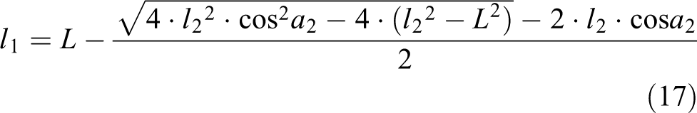
As the distance between two adjacent two points is L, and a ₃ advances in the direction of distal section, therefore, l ₁ + l_t ₂ = L, l ₂ = Δp.

Calculation starts from the end link, solving each triangle, l ₁ can be figured out as equation (17)

l_{1} = L - \frac{\sqrt{4 \cdot l_{2} ​^{2} \cdot {cos}^{2} a_{2} - 4 \cdot (l_{2} ​^{2} - L^{2})} - 2 \cdot l_{2} \cdot cos a_{2}}{2}

When the manipulator has n sections, the above algorithm can also be used for calculation, and equation (17) can be written as equation (18)

l_{n} = L - \frac{\sqrt{4 \cdot l_{n + 1} ​^{2} \cdot {cos}^{2} a_{n + 1} - 4 \cdot (l_{n + 1} ​^{2} - L^{2})} - 2 \cdot l_{n + 1} \cdot cos a_{n + 1}}{2}

After solving each triangle, the new backbone line b ₀–b ₁–b ₂–b ₃…can be obtained using homogeneous coordinate transformation as equation (19). [p_an ] is the joint position in the original trajectory, and [p_bn ] is the joint position in the new trajectory

[\begin{matrix} p_{b n x} \\ p_{b n y} \\ p_{b n z} \\ 1 \end{matrix}] = [\begin{matrix} n_{a n x} & o_{a n x} & a_{a n x} & p_{a n x} \\ n_{a n y} & o_{a n y} & a_{a n y} & p_{a n y} \\ n_{a n z} & o_{a n z} & a_{a n z} & p_{a n z} \\ 0 & 0 & 0 & 1 \end{matrix}] \cdot [\begin{matrix} 0 \\ l_{n} \\ 0 \\ 1 \end{matrix}]

After the coordinates of each joint of the new configuration are acquired, the last step is to calculate the bending angles of each section. The two bending angles of each section can be solved according to joints positions to joint space kinematics in the “Joints positions to configuration space kinematics analysis” section. Thus, when the manipulator advance along the desired path for a certain distance, the new backbone line and its corresponding arrangement can be calculated using the geometric method. At this point, a single step has been calculated, for the next, the tip of the manipulator should advance Δ_tip * 2 until target point G is reached.

This process can be written as equation (20), in which config stands for the current backbone line and target stands for the target point for the manipulator to reach. When the calculation for reaching target point is done, the new arrangements are carried out, which include the bending angles and the displacement of the base for each step.

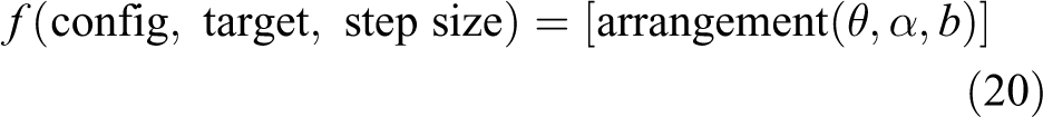
f (config, target, step size) = [arrangement (θ, α, b)]

Thus, the tip-follow process of Figure 8 can be written as equation (21)

f (config, target, step size) = f (config (a_{0}, a_{1}, a_{2}, a_{3}), G, Δ_{tip})

Advancing manipulator in predefined direction

The manipulator can also advance toward the predefined direction to the target point. In some confined space, this allows the manipulator to achieve sharp curves quicker, the operator can bend the distal section and advance the manipulator at the same time to approach the target point faster, but it may lead to a risk of collision as the distal section will not advance in a straight line. As shown in Figure 9, assuming that the manipulator has two sections, point a ₀ is the joint of the base and the first section, a ₂ is the tip of the distal section, and a ₀–a ₁–a ₂ is the backbone line of current arrangement of the manipulator. The target point is G, G–a ₂ and distal section a ₁–a ₂ form a certain angle.

Figure 9.

Solving new arrangement when advancing manipulator in predefined direction.

New arrangement can be obtained using the same method in the last section. Firstly, the inflection point in backbone line of the new configuration should be calculated. According to the orientation matrix of a ₂–G, then coordinate of b ₂ can be figured out using equation (19). After that, the coordinate of b ₀ and b ₁ can be calculated by solving triangles using the same method in the last section. At last, the two bending angles of each section can be solved according to joints positions to joint space kinematics in the “Joints positions to configuration space kinematics analysis” section.

The tip-follow process in Figure 9 can be written as equation (22)

f (config, target, step size) = f (config (a_{0}, a_{1}, a_{2}), G, Δ_{tip})

Path following method

The follow-the-leader methods stated in the “Advancing manipulator in the direction of tip” and “Advancing manipulator in predefined direction” sections use manipulator’s own backbone line as the target trajectory, and it is particularly suitable for the manual control of the manipulator when combined with machine vision. If the manipulator needs to follow a predefined path, one method is to fit backbone line with the desired curve. But the desired curve may be difficult to describe by mathematical expression, and this method will cost too much computation time.

The geometric approach of follow-the-leader method can also be applied to following a predefined path. If a path can be divided into adjacent points, follow-the-leader method can be used to follow the predefined path. The path which can be followed is determined by the length and maximum bending angle of the manipulator.

As shown in Figure 10, some feature points in the sine curve are extracted as target points,which can been seen as the process of curve discretization. The aim of path following method is to generate new arrangements for the manipulator to pass through each point.

Figure 10.

Following a sine curve using follow-the-leader method.

To achieve better follow-the-leader performance, the distances between target points may be different for some curves and may not be the same as the length of the links. The smaller the distance between the selected target points, the smaller the deviation from ideal path.

A new method for generating new path when following a predefined curve is proposed. As shown in Figure 11, a_n –a_n ₋₁–a_n ₋₂ is moving along G_m –G_m ₋₁–G_m ₋₂–G_m ₋₃ to reach target point G_m . The distance between each two joints is L, and it is longer than the distance between two adjacent target points. As the coordinates of a_n are already known, to find a_n ₋₁ is to find a point with a distance of L from a_n in G_m –G_m ₋₁–G_m ₋₂–G_m ₋₃. If |a_nG_m ₋₂| < L and |a_nG_m ₋₃| > L, a_n ₋₁ must be on G_m ₋₂–G_m ₋₃.

Figure 11.

Solving new arrangements when moving along a predefined curve.

In $△ a_{n} G_{m} _{- 2} G_{m} _{- 3}$ , using cosine theorem, equation (23) is acquired

cos b_{n - 1} = \frac{{| a_{n} G_{m - 3} |}^{2} + {| G_{m - 2} G_{m - 3} |}^{2} - {| a_{n} G_{m - 2} |}^{2}}{2 \cdot | a_{n} G_{m - 3} | \cdot | G_{m - 2} G_{m - 3} |}

Then in Δ a_na_n _-1 G_m _-3, equation (24) can be obtained using cosine theorem

L^{2} = {| a_{n} G_{m - 3} |}^{2} + {| a_{n - 1} G_{m - 3} |}^{2} - 2 \cdot | a_{n} G_{m - 3} | \cdot | a_{n - 1} G_{m - 3} | \cdot cos b_{n - 1}

|a_n ₋₁ G_m ₋₃| can be calculated as equation (25) by solving equation (24)

| a_{n} G_{m - 3} | = | a_{n - 1} G_{m - 3} | \cdot cos b_{n - 1} - \sqrt{{| a_{n - 1} G_{m - 3} |}^{2} \cdot {cos}^{2} b_{n - 1} - 4 \cdot {| a_{n} G_{m - 3} |}^{2} + 4 \cdot L^{2}}

Finally, the coordinate of a_n ₋₁ can be acquired as equation (26) through the slope of G_m ₋₃–G_m ₋₂ and coordinate of G_m ₋₃

a_{n - 1} = G_{m - 3} + \frac{G_{m - 2} - G_{m - 3}}{| G_{m - 2} G_{m - 3} |} \cdot | a_{n} G_{m - 3} |

The remaining points of the backbone line can be calculated as the same method in equations (23) to (26). The algorithm for finding new paths is a process of constantly comparing, solving triangles, and finding new points. The algorithm can be represented by the pseudo-code in Figure 12.

Figure 12.

Pseudo-code for solving new arrangement.

The complete follow-the-leader system

A flowchart of how the follow-the-leader method works is shown in Figure 13. In the block labeled (a), all the parameters are initialized, such as the number of sections, and the ideal follow-the-leader path is generated; then the system extracts one target point in order and solves the new configuration using geometric method in the block labeled (b); then the system goes back to extract the next target point, until all the target points are calculated, and comes to (c), new arrangements will be given to the manipulator and recorded. The cycle then repeats from input command. If the user wants to retract the manipulator, previous arrangements will be extracted from the database of historical arrangements and sent to the manipulator in the block labeled (d).

Figure 13.

Flowchart of the complete follow-the-leader method.

Simulation trials and results

To verify the algorithm and analyze the path deviation, the simulations of follow-the-leader method are carried out in MATLAB©(2018a). The simulations are performed on a desktop with an INTEL© i7-6700 processor, and results show that calculation time for per step is less than 0.5 ms.

Simulation of follow-the-leader navigation

Follow-the-leader method of serpentine manipulator can be realized by manual control under machine vision. With a camera embedded in the end-effector, the user can easily navigate the manipulator through a joystick by controlling the direction of the distal section and advance or retract of the manipulator according to the obstacle and target images from the camera. Figure 14 is the simulation results of a 10-section serpentine manipulator getting into the target chamber using follow-the-leader method. From 1 to 3, the manipulator bends toward the target while advancing using the method in the “Advancing manipulator in predefined direction” section. From 3 to 6, the manipulator bends toward the opposite direction while approaching the target. For the distal section may not be exactly aligned with the entrance of the chamber, the position of the distal section can be adjusted using inverse kinematics in 6 to 7. At last, in 7 to 8, the manipulator enters the chamber along the direction of the distal link using the method in the “Advancing manipulator in the direction of tip” section.

Figure 14.

Simulation of getting into a chamber using the follow-the-leader method.

The simulation totally has 500 steps, the computation time measured in MATLAB© is 220 ms, and the average time for a step is 0.44 ms. Due to geometric method, the computation time for each step is almost the same. Compared with the 12-section continuum manipulator using sequential quadratic programming optimization approach,¹⁷ in which the maximum computation time for a step is 2.3 s, with an average time of 0.391 s, the computation time of geometric method is much shorter. The number of sections is approximately linear with the calculation time, which means that the method can be applied to robots with a great number of sections without heavy computational load.

Comparison of different follow-the-leader methods

To verify the advantages of the geometric approach for follow-the-leader motion, a different follow-the-leader method is compared in this section.

FABRIK¹⁹ is a heuristic method for solving inverse kinematics problem for articulated figures, which can also be used to generate follow-the-leader motion for serpentine manipulator. As shown in Figure 15(a), the initial position of the manipulator is a ₀–a ₁–a ₂–a ₃ and the target point is G. Move the end effector a ₃ to G and mark it as b ₃. Then find the joint b ₂ which lies on the line that passes through the points b ₃ and a ₂ and has distance L from the joint b ₃ and continue the algorithm for the rest of the joints. The advantage of the FABRIK method is the low computational cost, but the deviation of the overall configuration of the manipulator is relatively large compared with the joint configuration generated by the follow-the-leader method in this article as shown in Figure 15(b). Another problem of FABRIK is that the base denoted by b ₀ is not on the line a ₀–a ₁, which indicates that the base of the manipulator leaves the horizontal position, it is impossible for a manipulator mounted on a linear guide rail.

Figure 15.

Illustration of geometric approach for follow-the-leader motion: (a) FABRIK method (b) follow-the-leader method.

Follow-the-leader method can also be used in continuum manipulator,¹⁷ as it has different mechanical structure from rigid-backbone manipulator, the path deviations are also different for them. As shown in Figure 16(a), it can be seen that there is no error for the tip position of the serpentine manipulator. However, in Figure 16(b), there is an oscillating error e (=0.136L) in the tip position of the continuum manipulator, when the manipulator is operated with camera in the distal section, it may cause problem to the images from the camera. As a result, the serpentine robot has no error for the tip position when carrying out follow-the-leader motion, but it needs more sections to realize complex pose compared with continuum robot.

Figure 16.

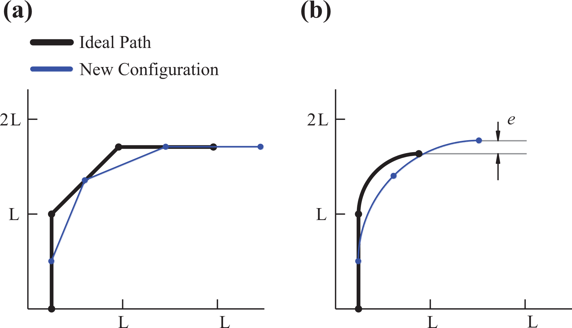
Deviation from ideal path of serpentine robot and continuum robot: (a) serpentine robot (b) continuum robot.

Analysis of deviation from the ideal path

As the serpentine manipulator consists of discrete links, its new arrangement cannot meet the ideal path completely when carrying out follow-the-leader motion. The deviation from the ideal path is analyzed in this section.

Error analysis of a single section is shown in Figure 17. a–b is a single section of the new arrangement, and δ is the deviation from the ideal path. As the manipulator is operated in the follow-the-leader method, a–b is siding on the ideal path. When α = θ/2, deviation δ reaches the maximum.

Figure 17.

Maximum deviation of single section.

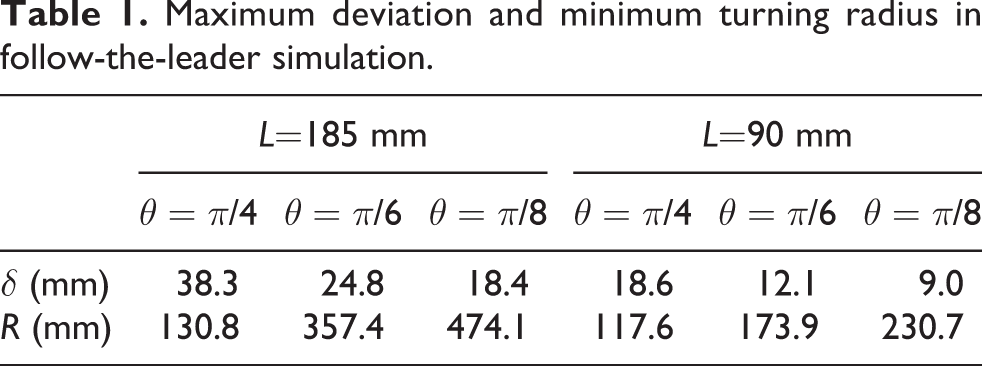
Maximum deviation can be calculated by equation (27), which is related to the bending angle and the section length. In the simulation, L = 185 mm, θ = π/6, maximum deviation δ is 24.8 mm. In consideration of the diameter of each section, the maximum deviation δ′ is the same as δ

δ = \frac{L}{2} \cdot tan (\frac{θ}{2})

By overlaying each of these arrangements, it creates an envelope which provides a visualization of the deviations and where they occur. Figure 18 is S-bend profiles, S-bends consist of two bends and return the tip to the initial orientation. When the length of section L comes to 90 mm, the envelope area of the path is obviously reduced, compared with L of 185 mm. From the simulation result, it is easily known that, when the manipulator is advancing in the direction of tip, there is no deviation in the tip position and maximum deviation occurs at the joints.

Figure 18.

S-bend profiles. (a) longer section length with larger deviation, L = 185mm, θ = pi/6, δ = 24.8mm (b) shorter section length with smaller deviation, L = 90mm, θ = pi/6, δ = 12.1mm.

The minimum turning radius can also reflect the obstacle capability of the manipulator. The minimum turning radius can be calculated by equation (28), increasing the bending angle or reducing the section length can reduce the minimum turning radius of the manipulator

R = \frac{L / 2}{cos ((π - θ) / 2)}

Figure 19 shows π/2 profiles of the manipulator, and it can be seen that the larger the bending angle, the smaller the minimum turning radius.

Figure 19.

π/2 profiles.

Table 1 shows maximum deviation and minimum turning radius with different section lengths and maximum bending angle.

Table 1.

Maximum deviation and minimum turning radius in follow-the-leader simulation.

	L=185 mm			L=90 mm
	θ = π/4	θ = π/6	θ = π/8	θ = π/4	θ = π/6	θ = π/8
δ (mm)	38.3	24.8	18.4	18.6	12.1	9.0
R (mm)	130.8	357.4	474.1	117.6	173.9	230.7

All the simulations in this section ignore the diameter of the manipulator, and the maximum bending angle is related to the design of the manipulator sections. When maximum bending angle becomes larger, the diameter of each section may increase and the central hole in each section may become smaller at the same time. That is to say, the capability of obstacle avoidance for a certain serpentine manipulator should take into account the section diameter and the actual structure of the manipulator.

Demonstration on physical hardware

An experimental platform is built to validate the kinematics model and the follow-the-leader method.

Experimental setup

The manipulator is driven by 18 servomotors with rated power of 80 W, and the motors are controlled by motor drivers which are connected to industry personal computer (IPC) via controller area network (CAN) bus. The experiment is performed based on the developed kinematics models and follow-the-leader method. The prototype of the manipulator has six sections, each section is 185 mm in length, and the maximal rotation angle of each section is 30°. The control system of the manipulator is briefly introduced here. When performing follow-the-leader motion, each step of the follow-the-leader motion will generate a new arrangement including the pitch angle, yaw angle of each section, and the displacement of the base. Then, the displacement of each driving cable can be obtained through the kinematics of the serpentine manipulator. According to the kinematics model, all the driving cables and the base must reach the new position at the same time. Thus, the displacement of the driving cables is converted into the displacement of the motors, and the speed of the motors is also calculated to make sure all the driving cables and the base reach the new position at the same time. After that, the displacement and speed of each motor are sent to the motor controller working in position mode through CAN bus. A timer in the control program will start waiting for the manipulator to reach the new arrangement and then come to the next arrangement.

To verify the simulation results and evaluate the follow-the-leader performance, two magnetic rotary encoders are embedded into each universal joint, which can measure the rotation angles of each section. The 14-bit encoder integrated circuit (IC) consists of Hall sensors, analog digital converter, and digital signal processing, which measures the absolute position of the magnet’s rotation angle. As shown in Figure 20, a magnet is fixed to the shaft, and the shaft is connected with the support through the flat position. Thus, the attitude of the manipulator can be measured through the rotation of the magnet relative to the encoder IC.

Figure 20.

Schematic representation of magnetic rotary encoder embedded in universal joint.

The encoder ICs are installed on small printed circuit boards attached to the center block of universal joint. As each universal joint has two encoder boards, there are totally 12 encoder boards in the manipulator. If each encoder board uses one ribbon cable to communicate with the IPC, it needs 12 channels and there will be too many cables going through the center blocks of the universal joints. To solve this problem, the encoder ICs use serial peripheral interface (SPI) and they are connected in daisy chain for serial data readout. As shown in Figure 21, encoder boards are connected in serial, there will be only one ribbon cable going through the manipulator, and all the angles data can be received by the IPC through one SPI channel.

Figure 21.

Illustration of encoders working in SPI daisy chain mode. SPI: serial peripheral interface

When the encoders work in SPI daisy chain mode, the data of 12 rotation angles will be latched simultaneously, and 24 bytes of data will be transmitted to IPC. The maximum sampling rates of the encoder IC are 11.25 kHz, and the IPC uses an SPI-USB adapter working in 12 MHz to communicate with it.

The theoretical sampling and transmission time are less than 0.1 ms, considering the stability and transmission capability of the system, the IPC reads the angle data every 50 ms.

Follow-the-leader navigation test

Follow-the-leader navigation test is carried out in manual control mode by a joystick. The user can control the bending of the distal section and the advance or retreat of the base. In Figure 22(a) and (b), distal section was bending up while advancing, in Figure 22(c) and (d), distal section was bending down while advancing, and the distal section came to a horizontal position. In Figure 22(e) and (f), the manipulator was advancing in the direction of the tip, distal section stayed in the horizontal position. Finally, in Figure 22(g) and (h), the manipulator retracted along the prior path.

Figure 22.

Follow-the-leader navigation test: (a)∼(b) distal section was bending up while advancing (c)∼(d) distal section was bending down while advancing (e)∼(f) the manipulator was advancing in the direction of the tip (g)∼(h) the manipulator retracted along the prior path.

The angular position data acquired from the sensors can be used to calculate the errors between actual trajectory and the path generated by the follow-the-leader method. According to the forward kinematics in the “Configuration space to task space kinematics analysis” section, the ideal and actual positions of each joint can be obtained, respectively, through the ideal angles generated from the follow-the-leader method and the measured angles. After that, the errors from the path generated by the follow-the-leader method of each section can be acquired in Figure 23. Due to error accumulation, the errors increase gradually from section 1 to section 6, and the maximum error is 6.25 mm. Due to the elasticity of the driving cable and the errors of assembly, errors for the tip position in actual operation cannot be avoided. Simulation results show that the manipulator can move along the path generated by the follow-the-leader method in real time.

Figure 23.

Errors of each section in follow-the-leader navigation.

Path following test

To verify the kinematics model and the follow-the-leader method, a helix path is set for the manipulator to follow. The helix curve is firstly dispersed into a line segments which have 40 target points and then generating follow-the-leader path through the process in the “Path following method” section. After that, the arrangement of each step can be calculated using the method in the “Joints positions to configuration space kinematics analysis” section.

As shown in Figure 24, path following test using the follow-the-leader method is performed on the experimental platform, and the corresponding feeding distance of the base is marked in the figure.

Figure 24.

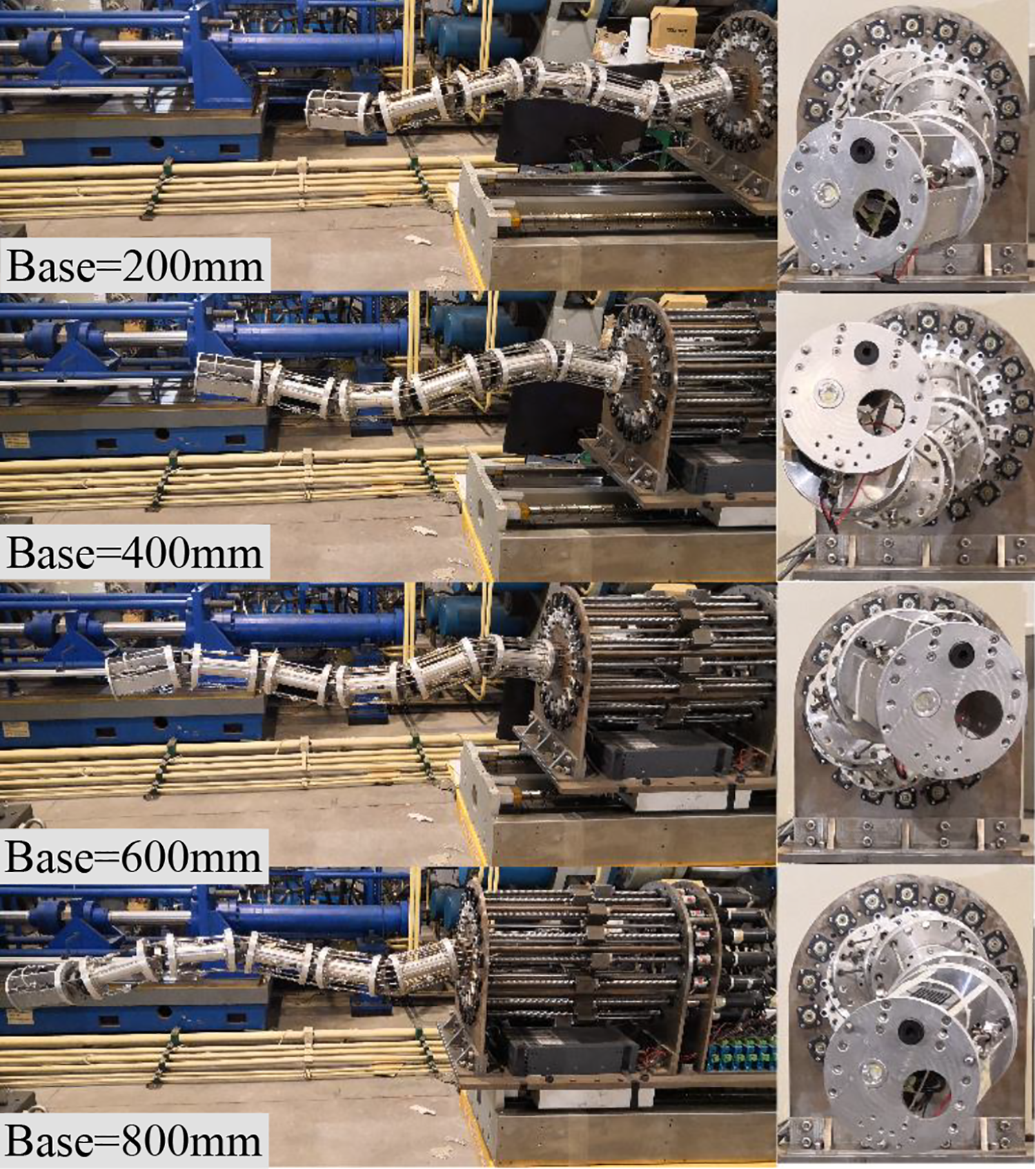
Following a helix curve using the follow-the-leader method.

Using the 12-axis encoders mentioned in the previous section, the six pitch angles and six yaw angles of the manipulator are collected every 50 ms. The result is shown according to the feeding distance of the base as shown in Figure 25

Figure 25.

Angle position collected from the 12 encoders when following a helix path.

Using the same method in the previous section, the errors from path generated by the follow-the-leader motion of each section can be acquired in Figure 26. Due to error accumulation, the errors increase gradually from section 1 to section 6, and the maximum error is about 12 mm. The results prove that the kinematics model and the path following method in the article are effective.

Figure 26.

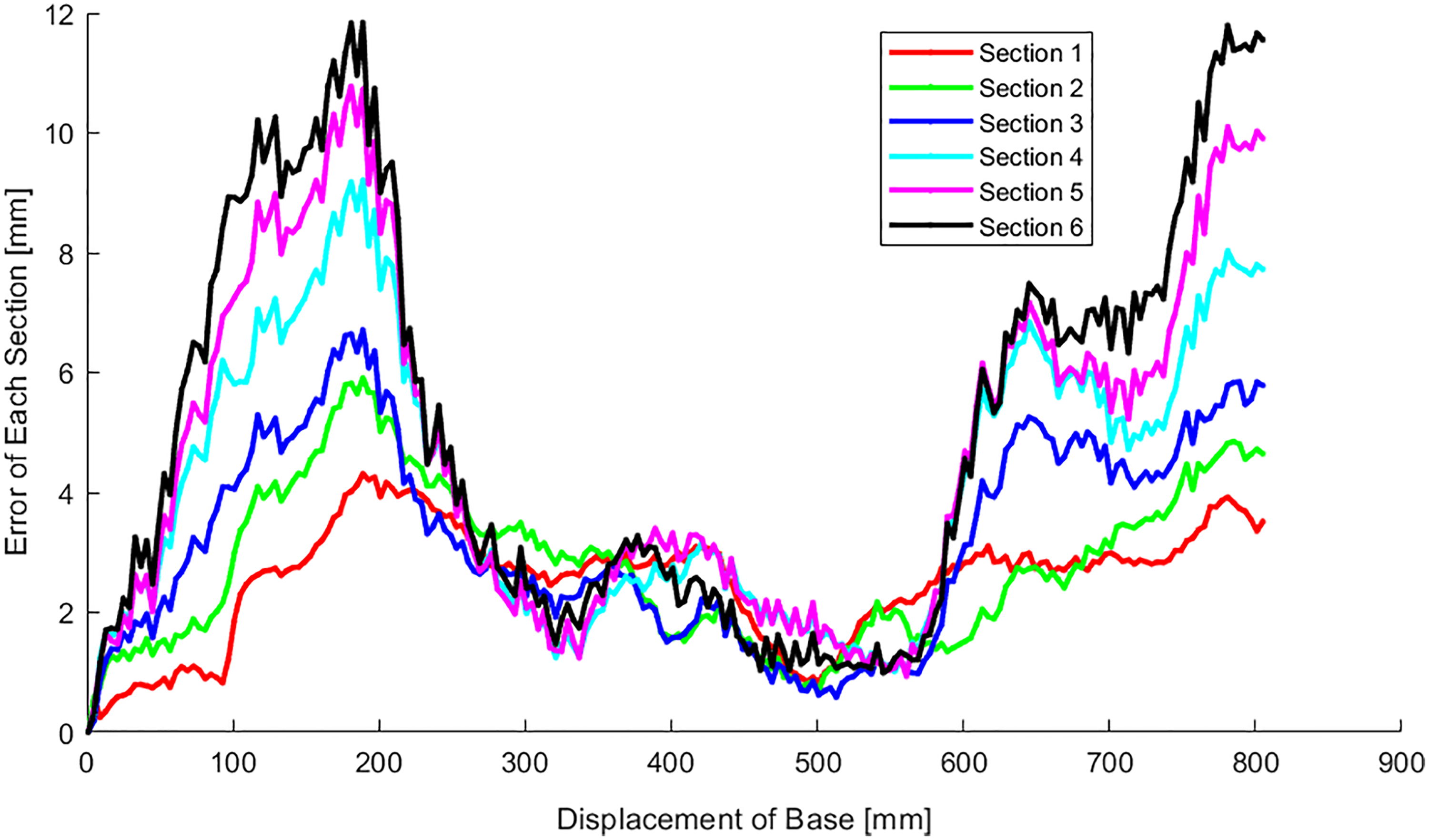
Errors of each section when following a helix path.

Experimental results and discussion

In the follow-the-leader navigation test, the maximum positioning error is 6.25 mm. For the path following test, the maximum positioning error is 12 mm. The errors analyzed in the simulation in the “Simulation trials and results” section are the inherent errors of the follow-the-leader method, when the maximum bending angle is π/6 and the length of section is 185 mm, the maximum deviation from the ideal path is 24.8 mm. While the errors measured in the experimental platform are the errors caused by factors such as elasticity of wire rope and assembly errors. Thus, the actual width of envelope of trajectory is larger than 24.8 mm and less than 24.8 mm + 12 mm in the path following test. According to the analysis in the “Comparison of different follow-the-leader methods” section, there is no theoretical error for the tip position when using the follow-the-leader method, therefore the actual error for the tip position is less than 12 mm during the path following process.

The first follow-the-leader experiment is carried out in manual mode under machine vision, which proves that the follow-the-leader method can perform interactive real-time path adjustment; in this way, the position and attitude of the manipulator can be controlled intuitively and rapidly.

In the second experiment, the manipulator is able to follow a predefined path with better end positioning accuracy, which means when the positions of obstacles and target location are determined, the follow-the-leader method can be used to follow a predefined path generated by the path searching algorithm.

Conclusions

This article represents a geometric method for follow-the-leader motion of cable-driven serpentine manipulator. When carrying out follow-the-leader motion, the tip of the manipulator is guided by the target points, and the manipulator will advance along the path that the tip has passed. As there is no theoretical error in tip position, follow-the-leader is suitable for manual control with a camera embedded in the end-effector, which greatly simplifies human–machine interaction. Moreover, the follow-the-leader method is also used to follow a predefined curve. By choosing any point on the curve as the target point, the manipulator will pass through these points in turn. Thus, the follow-the-leader method stated in this article can be applied to a variety of rigid-backbone serpentine manipulators for following a predefined 3-D path.

Simulation results show that calculation time for per step is less than 0.5 ms for serpentine manipulator with 10 sections. The calculation time of the geometric method is negligible compared with the numerical method, thus the method can be used to carry out real-time control. Experiments of follow-the-leader navigation and following a predefined path are also carried out to evaluate the performance of the method. Experimental results show that the manipulator can perform follow-the-leader motion well, and the deviation from the path is less than 12 mm when the manipulator follows a helix path.

Currently, the manipulator is working in open loop, and the positioning errors from ideal path are the main problem for the performance of follow-the-leader motion. The capability of obstacle avoidance is not totally analyzed when considering the diameter and design of the manipulator.

In the future, improving the accuracy of serpentine manipulator is the main objective. Using the angular position data collected from 12 encoders, feedback control can be carried out based on the dynamic models of serpentine manipulator. Moreover, the capability of obstacle avoidance should be further analyzed, based on the design of the serpentine manipulator. As the parameters of the manipulator restrict each other, optimum design of the manipulator can be further studied according to demand.

Footnotes

Declaration of conflicting interests

The author(s) declared no potential conflicts of interest with respect to the research, authorship, and/or publication of this article.

Funding

The author(s) received no financial support for the research, authorship, and/or publication of this article.

ORCID iD

Cheng Wang

References

Chirikjian

Burdick

. An obstacle avoidance algorithm for hyper-redundant manipulators. In: 1990 Proceedings, IEEE international conference on robotics and automation, Vol. 1, Cincinnati, Ohio, USA, 13–18 May 1990, pp. 625–631. IEEE.

Hannan

Walker

. The ‘elephant trunk’ manipulator, design and implementation. In: 2001 IEEE/ASME international conference on advanced intelligent mechatronics. Proceedings, vol. 1, Como, Italy, 8–12 July 2001, pp. 14–19. IEEE.

Hannan

Walker

. Kinematics and the implementation of an elephant’s trunk manipulator and other continuum style robots. J Field Robot 2003; 20: 45–63.

Walker

Hannan

. A novel ‘elephant’s trunk’ robot. In: 1999 IEEE/ASME international conference on advanced intelligent mechatronics. Proceedings, Atlanta, GA, USA, 19–23 September 1999, p. 410–415. IEEE.

Buckingham

. Snake arm robots. Ind Robot 2002; 29: 242–245.

Buckingham

Graham

. Snaking around in a nuclear jungle. Ind Robot Int J 2013; 32: 120–127.

Robinson

Davies

JBC

. Continuum robots—a state of the art. In: Proceedings 1999 IEEE international conference on robotics and automation, Vol. 4, Detroit, MI, USA, 10–15 May 1999, pp. 2849–2854. IEEE.

Festo Corporate. Bionic handling assistant—flexible and compliant movement. From bionic learning network. Festo Corporate, 2010, https://www.festo.com/group/en/cms/10241.htm.

Webster Iii

Jones

. Design and kinematic modeling of constant curvature continuum robots: a review. Int J Robot Res 2010; 29: 1661–1683.

10.

Asano

Obama

Arimura

, et al. Multijoint inspection robot. IEEE Trans Ind Electron 1983; 30: 277–281.

11.

Conkur

. Path following algorithm for highly redundant manipulators. Robot Auton Syst 2003; 45: 1–22.

12.

Bozek

Pokorny

Svetlik

, et al. The calculations of Jordan curves trajectory of the robot movement. Int J Adv Robot Syst 2016; 13: 1–7.

13.

Choset

Henning

. A follow-the-leader approach to serpentine robot motion planning. J Aerospace Eng 1999; 12: 65–73.

14.

William

II Mayhew

IV . Obstacle-free control of the hyper-redundant NASA inspection manipulator. In Proceedings of the fifth national conference on applied mechanics and robotics, Cincinnati, OH, 12–15, October 1997, pp. 12–15.

15.

Williams

. Follow-the-leader algorithm for the payload inspection and processing system. In: 1995 NASA/ ASEE Summer Faculty Fellowship Program, 1995, pp. 613–640.

16.

Neumann

Burgner-Kahrs

. Considerations for follow-the-leader motion of extensible tendon-driven continuum robots. In: IEEE international conference on robotics and automation, Stockholm, Sweden, 16–21 May 2016, pp. 917–923. IEEE.

17.

Palmer

Cobos-Guzman

Axinte

. Real-time method for tip following navigation of continuum snake arm robots. Robot Auton Syst 2014; 62: 1478–1485.

18.

Tappe

Pohlmann

Kotlarski

, et al. Towards a follow-the-leader control for a binary actuated hyper-redundant manipulator. In: IEEE/RSJ international conference on intelligent robots and systems, Hamburg, Germany, September 28–October 2 2015, pp. 3195–3201. IEEE.

19.

Aristidou

Lasenby

. FABRIK: a fast, iterative solver for the Inverse Kinematics problem. Graph Models 2011; 73: 243–260.

20.

Jones

Walker

. Kinematics for multisection continuum robots. IEEE Trans Robot 2006; 22: 43–55.

21.

Walker

Choset

Chirikjian

. Snake-like and continuum robots. Basel: Springer International Publishing, 2016.

22.

Chirikjian

Burdick

. Kinematics of hyper-redundant robot locomotion with applications to grasping. In: Proceedings. 1991 IEEE international conference on robotics and automation, Sacramento, CA, USA, 9–11 April 1991, pp. 781–793. IEEE.

23.

Ananthanarayanan

Ordóñez

. Real-time Inverse Kinematics of (2n + 1) DOF hyper-redundant manipulator arm via a combined numerical and analytical approach. Mech Mach Theory 2015; 91: 209–226.

A geometric approach for follow-the-leader motion of serpentine manipulator

Abstract

Keywords

Introduction

Mechanical design of the serpentine manipulator

Manipulator module design

Actuation system design

Kinematic modeling

Configuration space to task space kinematics analysis

Joints positions to configuration space kinematics analysis

Configuration space to actuator space kinematics analysis

Geometric approach for follow-the-leader motion

Advancing manipulator in the direction of tip

Advancing manipulator in predefined direction

Path following method

The complete follow-the-leader system

Simulation trials and results

Simulation of follow-the-leader navigation

Comparison of different follow-the-leader methods

Analysis of deviation from the ideal path

Demonstration on physical hardware

Experimental setup

Follow-the-leader navigation test

Path following test

Experimental results and discussion

Conclusions

Footnotes

Declaration of conflicting interests

Funding

ORCID iD

References