Model parameter estimation and residual life span prediction of pneumatic diaphragm pump based on hidden Markov model in intelligent spraying

Abstract

Pneumatic diaphragm pump is an important part in intelligent spraying. When pneumatic diaphragm pump does not work normally, the entire intelligent spraying product line will be malfunctioned. To maintain and manage pneumatic diaphragm pump effectively, the grade analysis of the health status of pneumatic diaphragm pump is generally used according to its working state. Due to the effects of condition monitoring and random faults, some observable health predictions are often inaccurate. There are very few papers dealing with the health monitoring of pneumatic diaphragm pump and their estimation of residual life span. In this article, a method with vector autoregressive model and continuous-time hidden Markov model was proposed to analyze and evaluate the life span of pneumatic diaphragm pump based on the estimation error of the health condition and the cumulative deterioration of pneumatic diaphragm pump. It is modeled through a continuous-time Markov chain with three states, which includes unobservable healthy state 0, unobservable warning state 1, and observable fault state 2. The expectation–maximization algorithm is used to estimate the model parameters of the fitted hidden Markov. Through the posterior probability of pneumatic diaphragm pump in warning state 1, the derived conditional reliability function and mean residual life span formula can be calculated to evaluate the residual life span of pneumatic diaphragm pump. The results showed that the method can effectively predict the residual life span of pneumatic diaphragm pump, illustrate the effectiveness of the model, and improve the accuracy of the health status rating.

Introduction

With the continuous development of the modern spraying process, the improvements of the spraying machine technology have made great progress. Nowadays, the requirements of the automated industrial production are gradually increasing, and the emergence of the spraying robot becomes inevitable. ^1,2 The painting robot is an industrial robot that can automatically paint or spray various coatings. Pneumatic diaphragm pump (PDP) is a safe machine because it is driven by compressed air. Moreover, the constant pressure of the pump output ensures the stable pressure requirement of spray micro atomization. Thus, PDP plays a vital role in the entire spraying system.

PDP is a new type of conveying machine. It has a good pumping effect on various corrosive, high-viscosity, highly toxic, and other liquids. Meanwhile, it owns similar advantages to self-priming pumps and centrifugal pumps. Diaphragm, as a critical part of the diaphragm pump, operates the virtue of piston pump such as simple and durable structure. On the other hand, rubber diaphragm, which is an important part of the PDP for propelling liquid, has higher abrasive and corrosion resistivity compared with other reciprocating pumps. The PDP is being widely used in various fields due to the recent developments in fretting corrosion resistance and corrosion resistance. It is able to use the diaphragm in the cylinder to agitate the work to achieve the purpose of conveying various liquids. ³

PDP is a complicated machine because of many internal parts. The fault of any part will affect the normal operation of PDP. ⁴ During the operation of PDP, the fault is very frequent such as diaphragm rupture or diaphragm elastic failure and inlet and outlet pipeline blockage. Once a component of the PDP fails, the PDP will not work properly. The quality of the already sprayed product cannot be up to the standard if the abnormal working state of the PDP cannot be found in time. This will cause some products to fail and need to be reworked, which is time-consuming and labor intensive. In addition, repairing or replacing a faulty PDP will delay the work of the entire production line. With data collection and computer technology, it is possible to implement an effective condition monitoring system for critical equipment so that the plant productivity is improved. ⁵ The goal is to use the information obtained from condition monitoring to assess the actual condition of the operating PDP without any unnecessary interruptions. In the presence of condition monitoring data, the primary predictive feature used in machine prediction is the mean residual life span (MRL), which represents the average remaining time before a fault occurs, given the current machine condition and past observations. Thus, timely and accurate monitoring of the working state of the PDP and the estimation of the residual life span (RL) of the PDP are of great significance for the safe production of the spray. ⁶

In recent years, the fault analysis of PDP has been widely studied. Yu et al. carried a simulation to the virtual prototype of the diaphragm pump based on the numerical value analyze software MATLAB 2014 a+ and the dynamics of mechanical system simulation software ADAMS 2010, 64 bits ⁷ ; Xu et al. developed an analytical model for the elastomeric diaphragm using the Mooney–Rivlin modeling method and elastomeric theory ⁸ ; Gong et al. presented a fault diagnosis of the high-pressure piston diaphragm pump based on acoustic emission. ⁹ However, few people have considered the effect of random fault on some observable systems as well as estimated the RL of PDP.

In this article, a statistical method is proposed to predict the RL of PDP. Statistical methodology is based on rigorous stochastic modeling and statistical analysis of available effective state monitoring information, so it is a common method in fault diagnosis. The specific implementation process is shown in Figure 1. There are three main statistical methods for early fault prediction using state monitoring information in industry: the proportional simulation modeling, stochastic recursive filtering, ¹⁰ and hidden Markov models (HMMs). ¹¹ HMM has been certified to be the most effective in progressive degradation system modeling and is widely used in many fields, such as speech and handwriting recognition, econometrics, and most recently, condition-based maintenance. ^12,13 The states of the system are identified as a three-state continuous-time Markov chain that collects real multivariate data, where state 0, state 1, and state 2 represent healthy state, warning state, and fault state, respectively. ^14,15 State 0 means that PDP is working properly and there is no tendency to malfunction. In state 1, PDP can operate normally, but there is a chance of malfunctioning. These two states are unobservable but can be estimated from the data obtained by monitoring system state. Gradually, the failure rate continues increasing and the system will enter state 2, at some time point PDP will no longer operate and no further state monitoring data will be collected, which is observable. ¹⁶

Figure 1.

HMM-based procedure for RL prediction. HMM: hidden Markov models; RL: residual life span.

After the establishment of the model, the study based on expectation–maximization algorithm (EMA) is applied to estimate the state and observation parameters of hidden Markov. ^17,18 The main advantage of this EMA compared with other maximum likelihood estimation methods is that it can be performed well even if some information or data are missing. ¹⁹ However, the state process in the HMM is unobservable, which makes the EMA particularly suitable for parameter estimation in the HMM framework. ²⁰ Estimating the parameters of HMM using EMA generally has two calculation methods. One method is to fit the vector autoregressive (VAR) model to the preprocessed historical data then to calculate the residual of the entire data history use the fitted model. The other method is to directly use the preprocessed historical data then to apply the observation process model and the state space representation of the Kalman filter. This study uses the residual obtained from the VAR as the observation process in the hidden Markov framework. Once the hidden Markov parameters are estimated, the RL of PDP can be predicted using the derived conditional reliability function (CRF) and the explicit formula of the MRL function of the posterior probability. ^21,22 The MRL function can be calculated using the posterior probability, indicating the average remaining time before the malfunction occurs by the current PDP condition and past observations. ^23,24 From the theory of the partially observable hidden Markov decision process, it can be derived that the posterior probability of PDP in the warning state is a univariate statistic, whereas the observation from the state sample is multidimensional vector data. ²⁵ In the field of fault prediction, hidden Markov is used to model the state deterioration process, and it is very novel to estimate the RL of PDP according to the deterioration condition. Moreover, the RL prediction of the HMM applied to PDP has not yet been completed currently.

The rest of this article is organized as follows. In the “Experimental platform construction and VAR model and residual calculation” section, the study will be executed about applying the VAR model to the data of the diaphragm’s motion frequency and outlet pressure in a PDP and obtaining both healthy and unhealthy residuals. In the “Hidden Markov modeling and estimation of parameters” section, the obtained residual is used as the observation process of HMM, and the model parameters are estimated by the EMA. In the “CRF and MRL functions for RL prediction” section, the CRF and the MRL function are used to predict the remaining life span of PDP. Conclusions and future perspectives are provided in the “Conclusions” section.

Experimental platform construction and VAR model and residual calculation

An abnormal continuation of the working condition occurs because of failure of PDP. Meanwhile, there are a series of changes in the variables of the pump, such as the frequency of movement of the diaphragm, the vibration amplitude of the pump, and the liquid pressure at the outlet. However, the motion frequency of PDP and the liquid pressure at the outlet will carry most of the fault information after the fault occurs. ⁹ For example, when the PDP is working normally, the number of times the cylinder diaphragm reciprocates in a unit time is kept within a certain range. If the number of times is not within the normal range, the PDP may have a malfunction such as blockage or diaphragm rupture. To avoid excessive parameterization, the two-dimensional (2-D) diagnostic data from the composition of the diaphragm pump’s diaphragm frequency and outlet fluid pressure were studied.

An experimental platform was built firstly to acquire data. The working power of PDP was provided by an air compressor with a stable pressure output (0.6 MPa). The main function of the program logic controller (PLC) is to obtain the state operation information of PDP, such as the motion frequency of the diaphragm and the pressure of the water at the outlet of PDP. The acquired status information was displayed on the personal computer through the application software, and the data were saved to a local database for further data analysis. Figure 2 shows the specific experimental platform.

Figure 2.

Construction of the experimental platform.

The data are acquired by the PLC and the sensor. Firstly, the proximity switch is placed at the position of the diaphragm drive shaft, and the magnetic ring of the drive shaft is sensed to record the motion frequency of the diaphragm. When the PDP reciprocates once, the proximity switch generates a switching signal. In addition, the pressure sensor is installed at the water outlet of the pump to obtain the pressure value of the water at the outlet. Figure 3 shows the specific location layout.

Figure 3.

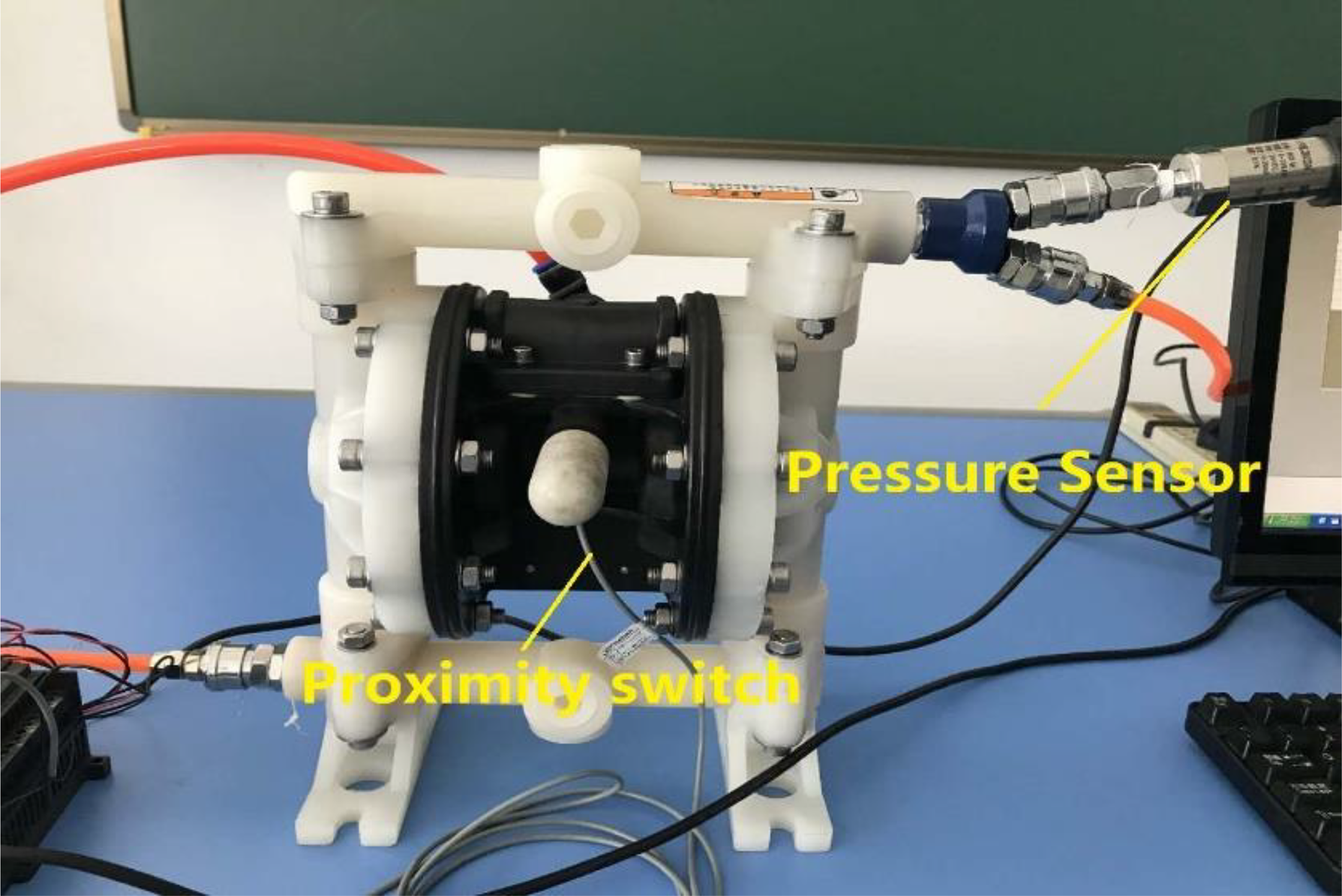
Sensor position on PDP experiment platform. PDP: pneumatic diaphragm pump.

Two types of data histories were considered. One is the end of PDP failure and the other is that PDP was halted without the end of the fault. The fault history is defined as the historical data of the end of the fault observed, indicating that PDP can no longer be used normally. The pause history is defined as the historical data of PDP while it is still running without losing its function. During the life span of PDP, the study performs a data acquisition and analysis of the data for PDP every 1 h. A total of three historical data are collected throughout the study. Figure 4 is a list of trends in diaphragm motion frequency and outlet pressure with respect to time over the life span of all three data histories.

Figure 4.

Trend graph of motion frequency and outlet fluid pressure.

It can be observed from Figure 4 that the measured value is stable from the first cycle to the 130th cycle. This indicates that PDP operates under normal conditions, and this part is considered to be a healthy part of historical data. After the 130th cycle, the diaphragm frequency value decreased significantly and the outlet pressure value increased significantly. This indicates that the entire working system is starting to operate abnormally, which is considered as an unhealthy part of historical data. For our experiments, the pressure value of the water at the outlet of PDP is a pulse value. As long as it fluctuates stably within a certain range, it can be regarded as normal condition, which explains the local fluctuation of the pressure trend of the outlet water in Figure 4.

Time series segmentation is the division of a nonstationary time series into a finite number of still parts. ^26,27 Sequence segmentation is for better processing of sequences. The segmentation in this study is to achieve a smooth history in the healthy part of the data, which in turn can identify the healthy part of the data history so that the static time series model can be fitted, and the residual model can be calculated using the simulation model. ²⁷ There are many ways to divide. In this study, only the historical data need to be divided into healthy and unhealthy parts. Since there is no basic “optimal” segmentation standard, for simplification, in this article, the data history is selected by graph check.

In all historical data, the healthy part of it is represented as $\left\{Z_1^l,\dots ,Z_{tl}^l\right\},l=1,\dots ,N+M$ .

We assume that health data follow a common VAR process as follows

$Z_n-{{\displaystyle \delta }}_0={\displaystyle \sum _{r=1}^p{{\displaystyle \Phi }}_r}\left(Z_{n-r}-{\delta }_0\right)+{\epsilon }_n,n\in Z$

1

where ε _n are i.i.d. N₂(0, C), p ∈ N is the model order, Φ_r ∈ R^2×2 is the autocorrelation matrices and δ ₀ ∈ R² and C ∈ R^2×2 is the mean and covariance model parameters. To make the health data history $\left\{Z_1^l,\dots ,Z_{tl}^l\right\},l=1,\dots ,N+M$ have a regression representation W = VA + E, which is used to indicate that δ is used to represent $\delta \text{=}{\delta }_0-{\displaystyle {\sum }_{r=1}^p{{\displaystyle \Phi }}_r}{{\displaystyle \delta }}_0$ .

Where

$W\text{'}\text{=}\left[{{\displaystyle Z}}_{{{\displaystyle t}}_{N+M}}^{N+M}\mathrm{...}{{\displaystyle Z}}_{p+1}^{N+M}\mathrm{...}{{\displaystyle Z}}_{{{\displaystyle t}}_1}^l\mathrm{...}{{\displaystyle Z}}_{p+1}^l\right],A\text{'}\text{=}\left[\delta ,{{\displaystyle \Phi }}_{\text{1}}\mathrm{...}{{\displaystyle \Phi }}_p\right],E\text{'}\text{=}\left[{{\displaystyle \epsilon }}_{{{\displaystyle t}}_{N+M}}^{N+M}\mathrm{...}{{\displaystyle \epsilon }}_{p+1}^{N+M}\mathrm{...}{{\displaystyle \epsilon }}_{{{\displaystyle t}}_1}^l\mathrm{...}{{\displaystyle \epsilon }}_{p+1}^l\right]$

${{\displaystyle V}}^{\text{'}}=\left[\begin{array}{cccc}1& 1& 1& 1\\ {{\displaystyle Z}}_{{{\displaystyle t}}_{N+M}-1}^{N+M}& {{\displaystyle Z}}_p^{N+M}& {{\displaystyle Z}}_{{{\displaystyle t}}_{N+M}-1}^l& {{\displaystyle Z}}_p^l\\ ⋮& ⋮& ⋮& ⋮\\ {{\displaystyle Z}}_{{{\displaystyle t}}_{N+M}-1}^{N+M}& {{\displaystyle Z}}_1^{N+M}& {{\displaystyle Z}}_{{{\displaystyle t}}_{N+M}-p}^l& {{\displaystyle Z}}_1^l\end{array}\right]$

The following is the least squares estimate for A and C

$\widehat{A}={{\displaystyle \left(V\text{'}V\right)}}^{-1}{{\displaystyle V\text{'}V}}^{},\widehat{{\displaystyle C}}={{\displaystyle \left(T-\left(2\text{p}+1\right)\right)}}^{-1}{{\displaystyle \left(W-V\widehat{A}\right)}}^{\text{'}}\left(W-V\widehat{A}\right),T={\displaystyle \sum _{\text{l}=1}^{N+M}\left({{\displaystyle t}}_1-p\right)}$

2

where T is the total number of available data points. The parameters of these models are unknown and need to be estimated. The estimation of model order p ∈ N is obtained by testing H ₀: Φ _p = 0 against H _a: Φ _p ≠ 0 using the likelihood ratio statistic given by

${{\displaystyle M}}_p=-\left({{\displaystyle T}}_{}-{{\displaystyle 2p}}^{}-{{\displaystyle 1}}^{}-\frac{{{\displaystyle 1}}_{}}{{{\displaystyle 2}}_{}}\right){{\displaystyle \text{ln}}}_{}\left(\frac{{{\displaystyle \text{det}}}_{}\left({{\displaystyle S}}_p\right)}{{{\displaystyle \text{det}}}_{}\left({{\displaystyle S}}_{p-1}\right)}\right)$

3

where Sp is the remaining sum of squares, the specific expression is as follows

${{\displaystyle S}}_{\text{p}}=\left(W-V\widehat{A}\right)\text{'}\left(W-V\widehat{A}\right)$

For the actual 2-D pump data, M ₂ = 10.8923 and M ₃ = 5.5229 can be obtained by the above formula. From the χ² distribution with two degrees of freedom and α = 0.05, ${\chi }_{2,0.05}^2=5.99$ . Since $M_2>{\chi }_{2,0.05}^2$ and $M_3<{\chi }_{2,0.05}^2$ , we reject H ₀: Φ₂ = 0 and fail to reject H _a: Φ₃ = 0. So $\widehat{P}=2$ is a suitable model order, and the parameter estimate of the VAR model can be derived by equation (2)

$\widehat{P}=2\widehat{{\displaystyle C}}=\left(\begin{array}{cc}{{\displaystyle 9.5707e+2}}_{}& {{\displaystyle -1.1195e-1}}_{}\\ {{\displaystyle -1.1195e-1}}_{}& {{\displaystyle 1.1098e-3}}_{}\end{array}\right)$

${{\displaystyle \widehat{\Phi }}}_{\text{1}}\text{=}\left(\begin{array}{cc}{{\displaystyle \text{6.7096}e-1}}_{}& {{\displaystyle 2.4379e+2}}_{}\\ {{\displaystyle 1.7483e-4}}_{}& {{\displaystyle 6.9158e-2}}_{}\end{array}\right){{\displaystyle \widehat{{\displaystyle \Phi }}}}_{\text{2}}\text{=}\left(\begin{array}{cc}{{\displaystyle 3.3254e-1}}_{}& {{\displaystyle 4.6590e-1}}_{}\\ {{\displaystyle -3.6843e-4}}_{}& {{\displaystyle 3.2061e-1}}_{}\end{array}\right)$

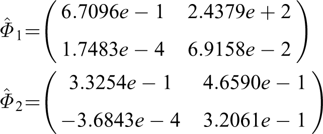
With the estimate $\widehat{\gamma }=\left(\widehat{\delta },\widehat{P},{\widehat{\text{Φ}}}_1,{\widehat{\text{Φ}}}_2,\widehat{C}\right)$ , the residual process is defined as

${{\displaystyle Y}}_n:={{\displaystyle Z}}_n-{{\displaystyle E}}_{\widehat{y}}\left({{\displaystyle Z}}_n|\overrightarrow{{{\displaystyle Z}}_{\text{n-1}}}\right)$

4

where

$\overrightarrow{{{\displaystyle Z}}_{\text{n-1}}}\text{=}\left({{\displaystyle Z}}_{\text{1}},\mathrm{...},{{\displaystyle Z}}_{n-1}\right)$

The calculation method of the residual calculation formula (4) is given in the literature, ^24,27 whereby the residuals of the healthy part and the unhealthy part in the historical data can be calculated. The residual is given as a 2-D scatter plot, as shown in Figure 5. The blue dots indicate the residual calculated from the healthy portion of the pump historical data, whereas the orange dots represent the residual calculated from the unhealthy portion of the pump historical data.

Figure 5.

Residual two-dimensional scatter plot of historical data.

The ultimate goal of this article is to model the state process of a PDP and to evaluate the remaining life span of PDP with the configured model. After the data preprocess through historical data segmentation and VAR modeling, the residuals will be obtained from the observation process. The hidden Markov parameters are estimated in the following text. Then the established model will be used to evaluate the RL of PDP.

In the next section, the residual is to be used as the hidden Markov observation process, and the EMA will be used to estimate the hidden Markov state and observation parameters.

Hidden Markov modeling and estimation of parameters

In this section, the residual data are considered to be a part of the observed data to fit the HMM. ²⁸ The state of PDP is divided into good state (state 0), warning state (state 1), and fault state (state 2), and only the fault state is observable. This article models the state process (X_t : t ∈ R₊) as a continuous-time homogeneous Markov chain with a spatial state {0, 1, 2}. Assuming that PDP starts from a good state of health, that is, X ₀ = 0, the conversion rate matrix is as follows

${{\displaystyle \Lambda }}_{}\text{=}\left(\begin{array}{ccc}-\left({{\displaystyle \lambda }}_{01}+{{\displaystyle \lambda }}_{02}\right)& {{\displaystyle \lambda }}_{01}& {{\displaystyle \lambda }}_{02}\\ 0& -{{\displaystyle \lambda }}_{12}& {{\displaystyle \lambda }}_{12}\\ 0& 0& 0\end{array}\right)$

5

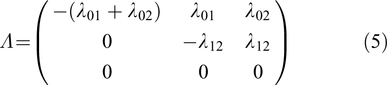
where λ ₀₁, λ ₀₂, λ ₁₂∈(0,+∞) are unknown model parameters and need to be estimated. Since the system deterioration needs to go through state 0 to state 1, and the probability of failure occurring in state 1 is high, the result is λ ₁₂ > λ ₀₂. ²⁹ The last row of equation (5) contains only zero elements because once the system enters the failure state 2, it cannot leave the state before being replaced, that is, P(Y_n = η|X_{n Δ} = 2) = 1, where η ≠ R² represents the fault signal. And for a stable system, the sum of all the elements of each row of the conversion rate matrix is zero. ³⁰

Considering the state of PDP, it is assumed that the above residual process (Y_n : n ∈ N) is conditionally independent. For all n ∈ N, the study assumes that Y_n is conditional on X_{n Δ} = χ, χ = 0, 1, following a binary normal distribution density function N₂(µ_χ , Σ _χ )

${{\displaystyle f}}_{{{\displaystyle Y}}_n|{{\displaystyle X}}_{n\Delta }}\left({{\displaystyle y}}_{}|{{\displaystyle \chi }}_{}\right)=\frac{1}{\sqrt{{{\displaystyle \left(2\pi \right)}}^2{{\displaystyle \text{det}}}_{}\left({{\displaystyle \Sigma }}_{\chi }\right)}}{{\displaystyle \text{exp}}}_{}\left(-\frac{1}{2}\left({{\displaystyle y}}_{}-{{\displaystyle \mu }}_{\chi }\right)\text{'}{\displaystyle {\sum }_{\chi }^{-1}\left({{\displaystyle y}}_{}-{{\displaystyle \mu }}_{\chi }\right)}\right)$

6

where µ ₀, µ ₁ ∈ R² and Σ₀, Σ₁ ∈ R^2×2 are unknown observation parameters.

Where F_i and S_j are used to represent the fault history and pause history, respectively, and ξ = inf{t ∈ R₊: X_t = 2} is used to represent the observable failure time, where i ∈ [1, N], j ∈ [1, M]. Assuming that the fault history F_i has the form of $Y_i=\left(y_1^i,\dots ,y_{Ti}^i\right)$ and ξ_i = t_i , where T_i Δ ≤ t_i ≤ (T_i + 1)Δ. The sampling history Y_i represents the set of all data points of yⁱ _j ∈ R² (j ≤ T_i ), which is obtained when PDP fails at time t_i . Similarly, assuming that the pause history has the form of $Y_j=\left(y_1^j,\dots ,y_{Tj}^j\right)$ and ξ_j > T_{j Δ}. In this article, all observable data are represented by $O=\left\{F_1,\dots ,F_N,S_1,\dots ,S_M\right\}$ , and the correlation likelihood function is represented by L(λ, θ|O), where λ = (λ ₀₁, λ ₀₂, λ ₁₂) and θ = (µ ₀, µ ₁, Σ₀, Σ₁) are sets of unknown state parameters and observation parameters, which needs to be estimated. ³¹

Since the sample path of the state process is unobservable, the maximum correlation likelihood function cannot be analyzed. ³² Thus, the research solves this problem by means of EMA. EMA is very suitable to solve the parameter estimation problem of HMM and iteratively maximizes pseudo-likelihood function to estimate unknown parameters. The EMA consists of two steps: an E-step and an M-step. The E-step is to calculate the expectation of the correlation likelihood function, and the M-step to obtain the maximization of the unknown state and the observation parameters. Specific steps are as follows:

It is assumed that λ, θ are the initial values of the unknown state parameter and the observed parameter, respectively, and $\widehat{\lambda }$ and $\widehat{\theta }$ are estimates of unknown parameters from the M-step.

E-step: the pseudo likelihood function is defined by

${{\displaystyle Q}}_{}\left({{\displaystyle \lambda }}_{},{{\displaystyle \theta }}_{}|\widehat{{\displaystyle \lambda }},\widehat{{\displaystyle \theta }}\right):={{\displaystyle E}}_{\widehat{\lambda },\widehat{\theta }}\left(\text{ln}L\left({{\displaystyle \lambda }}_{},{{\displaystyle \theta }}_{}|{{\displaystyle C}}_{}\right)|{{\displaystyle O}}_{}\right)$

7

${{\displaystyle C}}_{}=\left\{{{\displaystyle \overline{F}}}_1,\mathrm{...},{{\displaystyle \overline{F}}}_N,\mathrm{...},{{\displaystyle \overline{S}}}_1,\mathrm{...},{{\displaystyle \overline{S}}}_M\right\}$

where C represents all data sets.

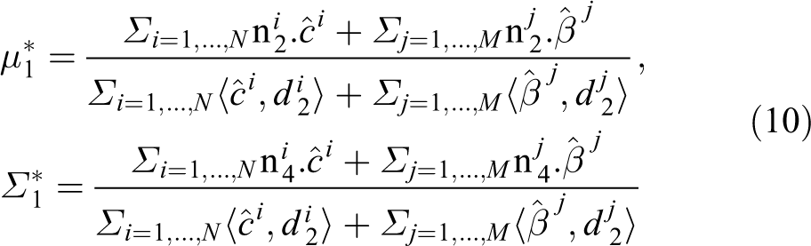
M-step: Calculate λ* and θ* according to the following formula

$\left({{\displaystyle \lambda }}^{*},{{\displaystyle \theta }}^{*}\right)\in \underset{{{\displaystyle \lambda ,\theta }}_{}}{{\displaystyle {{\displaystyle \text{argmax}}}_{}}}Q\left({{\displaystyle \lambda }}_{},{{\displaystyle \theta }}_{}|\widehat{{\displaystyle \lambda }},\widehat{{\displaystyle \theta }}\right)$

8

The calculated λ* and θ* are substituted as new parameters into the E-step, and the E-step and the M-step are repeated until the Euclidean norm $|({\lambda }^{*},{\theta }^{*})-(\widehat{\lambda },\widehat{\theta })|<\epsilon$ is satisfied, where ε is the selected stopping standard value.

The only maximization of the state parameters and observation parameters is given by the following formula

${{\displaystyle \lambda }}_{\text{01}}^{\text{*}}=-\frac{{\sum }_{i=1,\mathrm{...},N}{{\displaystyle \widehat{b}}}_{01}^i+{\sum }_{j=1,\mathrm{...},M}{{\displaystyle \widehat{\gamma }}}_1^j+\frac{{\sum }_{j=1,\mathrm{...},M}{{\displaystyle \widehat{\gamma }}}_2^j\left({\sum }_{\text{i}=\text{1,}\mathrm{...}\text{,}N}{{\displaystyle \widehat{b}}}_{01}^i+{\sum }_{j=1,\mathrm{...},M}{{\displaystyle \widehat{\gamma }}}_1^j\right)}{{\sum }_{i=1,\mathrm{...},N}{{\displaystyle \widehat{b}}}_{01}^i+{\sum }_{j=1,\mathrm{...}M}{{\displaystyle \widehat{\gamma }}}_1^j+{\sum }_{i=1,\mathrm{...},N}{{\displaystyle \widehat{b}}}_{02}^i}}{{\sum }_{i=1,\mathrm{...},N}{{\displaystyle \widehat{a}}}_{01}^i+{\sum }_{j=1,\mathrm{...},M}{{\displaystyle \widehat{\alpha }}}_{01}^j}$

${{\displaystyle \lambda }}_{\text{02}}^{\text{*}}={{\displaystyle \lambda }}_{\text{01}}^{\text{*}}\frac{{\sum }_{i=1,\mathrm{...},N}{{\displaystyle \widehat{b}}}_{02}^i}{{\sum }_{i=1,\mathrm{...},N}{{\displaystyle \widehat{b}}}_{01}^i+{\sum }_{j=1,\mathrm{...},M}{{\displaystyle \widehat{\gamma }}}_1^j},{{\displaystyle \lambda }}_{\text{12}}^{\text{*}}=-\frac{{\sum }_{i=1,\mathrm{...},N}{{\displaystyle \widehat{b}}}_{12}^i}{{\sum }_{i=1,\mathrm{...},N}{{\displaystyle \widehat{a}}}_{12}^i+{\sum }_{j=1,\mathrm{...},M}{{\displaystyle \widehat{\alpha }}}_{12}^j}$

9

and

${{\displaystyle \mu }}_0^{*}=\frac{{{\displaystyle \Sigma }}_{i=1,\mathrm{...},N}{{\displaystyle \text{n}}}_1^i.{\widehat{{\displaystyle c}}}^i+{{\displaystyle \Sigma }}_{j=1,\mathrm{...},M}{{\displaystyle \text{n}}}_1^j.{\widehat{{\displaystyle \beta }}}^j}{{{\displaystyle \Sigma }}_{i=1,\mathrm{...},N}〈{\widehat{{\displaystyle c}}}^i,{{\displaystyle d}}_1^i〉+{{\displaystyle \Sigma }}_{j=1,\mathrm{...},M}〈{\widehat{{\displaystyle \beta }}}^j,{{\displaystyle d}}_1^j〉},{{\displaystyle \Sigma }}_0^{\text{*}}=\frac{{{\displaystyle \Sigma }}_{i=1,\mathrm{...},N}{{\displaystyle \text{n}}}_{\text{3}}^i.{\widehat{{\displaystyle c}}}^i+{{\displaystyle \Sigma }}_{j=1,\mathrm{...},M}{{\displaystyle \text{n}}}_{\text{3}}^j.{\widehat{{\displaystyle \beta }}}^j}{{{\displaystyle \Sigma }}_{i=1,\mathrm{...},N}〈{\widehat{{\displaystyle c}}}^i,{{\displaystyle d}}_1^i〉+{{\displaystyle \Sigma }}_{j=1,\mathrm{...},M}〈{\widehat{{\displaystyle \beta }}}^j,{{\displaystyle d}}_1^j〉}$

${{\displaystyle \mu }}_1^{\text{*}}=\frac{{{\displaystyle \Sigma }}_{i=1,\mathrm{...},N}{{\displaystyle \text{n}}}_{\text{2}}^i.{\widehat{{\displaystyle c}}}^i+{{\displaystyle \Sigma }}_{j=1,\mathrm{...},M}{{\displaystyle \text{n}}}_{\text{2}}^j.{\widehat{{\displaystyle \beta }}}^j}{{{\displaystyle \Sigma }}_{i=1,\mathrm{...},N}〈{\widehat{{\displaystyle c}}}^i,{{\displaystyle d}}_{\text{2}}^i〉+{{\displaystyle \Sigma }}_{j=1,\mathrm{...},M}〈{\widehat{{\displaystyle \beta }}}^j,{{\displaystyle d}}_{\text{2}}^j〉},{{\displaystyle \Sigma }}_1^{\text{*}}=\frac{{{\displaystyle \Sigma }}_{i=1,\mathrm{...},N}{{\displaystyle \text{n}}}_{\text{4}}^i.{\widehat{{\displaystyle c}}}^i+{{\displaystyle \Sigma }}_{j=1,\mathrm{...},M}{{\displaystyle \text{n}}}_{\text{4}}^j.{\widehat{{\displaystyle \beta }}}^j}{{{\displaystyle \Sigma }}_{i=1,\mathrm{...},N}〈{\widehat{{\displaystyle c}}}^i,{{\displaystyle d}}_{\text{2}}^i〉+{{\displaystyle \Sigma }}_{j=1,\mathrm{...},M}〈{\widehat{{\displaystyle \beta }}}^j,{{\displaystyle d}}_{\text{2}}^j〉}$

10

Using equations (9) and (10), and the Euclidean norm stopping criterion $|({\lambda }^{*},{\theta }^{*})-(\widehat{\lambda },\widehat{\theta })|<{10}^{-4}$ , the results are presented in Table 1.

Table 1.

Iterations of the EMA.

	${{\displaystyle \lambda }}_{\text{01}}$	${{\displaystyle \lambda }}_{\text{02}}$	${{\displaystyle \lambda }}_{\text{12}}$	${{\displaystyle \mu }}_{\text{0}}$	${{\displaystyle \mu }}_{\text{1}}$	${{\displaystyle \Sigma }}_{\text{0}}$	${{\displaystyle \Sigma }}_{\text{1}}$
Initial values	0.0156	0	0.1170	$\left(\begin{array}{c}\text{2.5}e+1\\ -2e-2\end{array}\right)$	$\left(\begin{array}{c}-1e+1\\ -1.5e-1\end{array}\right)$	$\left(\begin{array}{cc}\text{9.6}e+2& -1.2e-1\\ -1.2e-1& 1.2e-3\end{array}\right)$	$\left(\begin{array}{cc}\text{9.6}e+2& -1.2e-1\\ -1.2e-1& 1.2e-3\end{array}\right)$
Optimal estimates	0.0078	0	0.0404	$\left(\begin{array}{c}2.04e+1\\ -1.766e-2\end{array}\right)$	$\left(\begin{array}{c}\text{6.832}e0\\ -6.07e-2\end{array}\right)$	$\left(\begin{array}{cc}\text{1.33}e+3& 6.18e-2\\ 6.18e-2& 2.072e-3\end{array}\right)$	$\left(\begin{array}{cc}\text{1.47}e+3& 2.26e-1\\ 2.26e-1& 4.68e-3\end{array}\right)$

EMA: expectation–maximization algorithm.

Then, the transfer rate matrix of equation (5) can be obtained as

$\Lambda \text{=}\left(\begin{array}{ccc}-0.0078& 0.0078& 0\\ 0& -0.0404& 0.0404\\ 0& 0& 0\end{array}\right)$

11

In Table 1, the article selects the initial value of the parameter through the experience of the predecessors. And subsequently iterates through the E step and the M step to obtain the parameter estimation value that satisfies the Euclidean norm. All calculations are coded in Python.

In the next section, based on the posterior probability of PDP in state 1, the study uses the estimated parameters of the model to calculate the CRF and the MRL function for the remaining life span of PDP.

CRF and MRL functions for RL prediction

In this section, the study will be based on the model CRF and the MRL proposed in the previous section to estimate the RL. Two of the formulas are functions of the posterior probability at the warning state (state 1).

Assuming that the uncertainty of the deterioration process of PDP follows the continuous-time homogeneous Markov chain (X_t : t ∈ R₊), and the state space is described as Z = {0, 1, 2}. State 0 and state 1 are unobservable operational states, and state 2 is an observable fault state. Because the posterior probability of PDP in the warning state is fully capable of helping the study achieve the final prediction, the study only needs to monitor the posterior probability of the warning state. The posterior probability of PDP in the warning state is expressed as

${{\displaystyle \Pi }}_n={{\displaystyle P}}_r\left({{\displaystyle X}}_{n\Delta }={{\displaystyle 1}}_{}|{{\displaystyle \xi }}_{}>{{\displaystyle n\Delta }}_{},{{\displaystyle Y}}_1,\mathrm{...},{{\displaystyle Y}}_n\right)$

12

where Δ represents the equidistant sampling time.

The Kolmogorov backward differential equation ³³ is solved by the aforementioned conversion rate matrix equation (5), and the following probability transfer matrix is obtained

$P(t)=\left[{{\displaystyle P}}_{ij}(t)\right]=\left[\begin{array}{ccc}{{\displaystyle e}}^{-\left({{\displaystyle \lambda }}_{01}+{{\displaystyle \lambda }}_{02}\right)t}& \frac{{{\displaystyle \lambda }}_{01}\left({{\displaystyle e}}^{-{{\displaystyle \lambda }}_{12}t}-{{\displaystyle e}}^{-\left({{\displaystyle \lambda }}_{01}+{{\displaystyle \lambda }}_{02}\right)t}\right)}{{{\displaystyle \lambda }}_{01}+{{\displaystyle \lambda }}_{02}-{{\displaystyle \lambda }}_{12}}& 1-{{\displaystyle e}}^{-\left({{\displaystyle \lambda }}_{01}+{{\displaystyle \lambda }}_{02}\right)t}-\frac{{{\displaystyle \lambda }}_{01}\left({{\displaystyle e}}^{-{{\displaystyle \lambda }}_{12}t}-{{\displaystyle e}}^{-\left({{\displaystyle \lambda }}_{01}+{{\displaystyle \lambda }}_{02}\right)t}\right)}{{{\displaystyle \lambda }}_{01}+{{\displaystyle \lambda }}_{02}-{{\displaystyle \lambda }}_{12}}\\ 0& {{\displaystyle e}}^{-{{\displaystyle \lambda }}_{12}t}& 1-{{\displaystyle e}}^{-{{\displaystyle \lambda }}_{12}t}\\ 0& 0& 1\end{array}\right]$

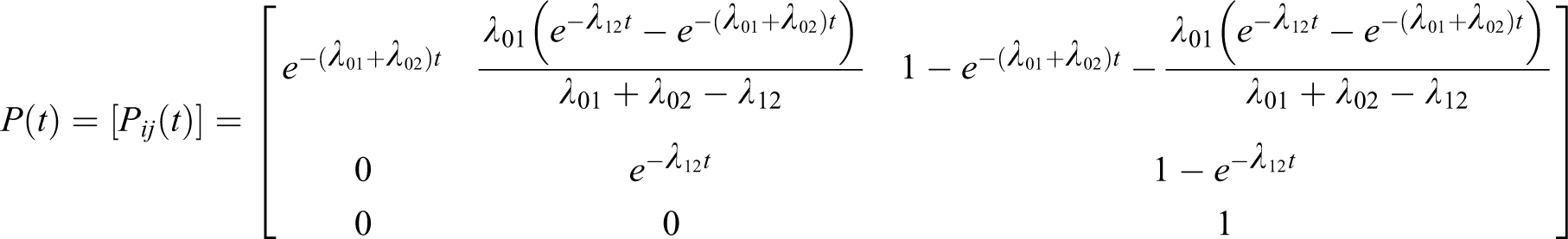
where the transition probabilities P_ij (t) = P(X_t = j | X ₀ = i), i, j∈[0, 1].

Using the Bayesian theorem n ≥ 1, the posterior probability can be recursively calculated as

${{\displaystyle \Pi }}_{n+\text{1}}=\frac{{{\displaystyle f}}_{{{\displaystyle Y}}_{n+1}|{{\displaystyle X}}_{(n+1)\Delta }}\left({{\displaystyle Y}}_{n+1}|1\right)\left({{\displaystyle P}}_{01}(\Delta )\left(1-{{\displaystyle \Pi }}_n\right)+{{\displaystyle P}}_{11}(\Delta ){{\displaystyle \Pi }}_{\text{n}}\right)}{{{\displaystyle f}}_{{{\displaystyle Y}}_{n+1}|{{\displaystyle X}}_{(n+1)\Delta }}\left({{\displaystyle Y}}_{n+1}|0\right)\left({{\displaystyle P}}_{00}(\Delta )\left(1-{{\displaystyle \Pi }}_n\right)+{{\displaystyle P}}_{\text{10}}(\Delta ){{\displaystyle \Pi }}_{\text{n}}\right)+{{\displaystyle f}}_{{{\displaystyle Y}}_{n+1}|{{\displaystyle X}}_{(n+1)\Delta }}\left({{\displaystyle Y}}_{n+1}|1\right)\left({{\displaystyle P}}_{01}(\Delta )\left(1-{{\displaystyle \Pi }}_n\right)+{{\displaystyle P}}_{\text{11}}(\Delta ){{\displaystyle \Pi }}_n\right)}$

where Π₀ = 0.

According to equation (6), the ratio of normal density can be derived as

$\frac{{{\displaystyle f}}_{{{\displaystyle Y}}_{n+1}|{{\displaystyle X}}_{(n+1)\Delta }}\left({{\displaystyle Y}}_{n+1}|{{\displaystyle 0}}_{}\right)}{{{\displaystyle f}}_{{{\displaystyle Y}}_{n+1}|{{\displaystyle X}}_{(n+1)\Delta }}\left({{\displaystyle Y}}_{n+1}|{{\displaystyle \text{1}}}_{}\right)}=\text{exp}\left({{\displaystyle \left({{\displaystyle Y}}_{n+1}-b\right)}}^{\text{T}}A\left({{\displaystyle Y}}_{n+1}-b\right)+c\right)h$

where

${{\displaystyle h}}_{}=\frac{{{\displaystyle |{\displaystyle \sum 0}|}}^{-1/2}}{{{\displaystyle |{\displaystyle \sum 1}|}}^{-1/2}}\hspace{1em}{{\displaystyle A}}_{}\text{=}\left(\frac{{\displaystyle {\sum }_{\text{1}}^{\text{-1}}}-{\displaystyle {\sum }_0^{\text{-1}}}}{{{\displaystyle \text{2}}}_{}}\right){{\displaystyle c}}_{}=\left(\frac{{{\displaystyle {{\displaystyle \mu }}^{\text{'}}}}_1{\displaystyle {\sum }_1^{-1}}{{\displaystyle \mu }}_1-{{\displaystyle {{\displaystyle \mu }}^{\text{'}}}}_0{\displaystyle {\sum }_0^{-1}}{{\displaystyle \mu }}_0}{{{\displaystyle 2}}_{}}\right)-{{\displaystyle b}}^{\text{T}}Ab$

${{\displaystyle b}}_{}=-\left(\frac{{{\displaystyle \left({\displaystyle {\sum }_0^{-1}}{{\displaystyle \mu }}_0-{\displaystyle {\sum }_1^{-1}}{{\displaystyle \mu }}_1\right)}}^{\text{'}}+{{\displaystyle \left({{\displaystyle {{\displaystyle \mu }}^{\text{'}}}}_0{\displaystyle {\sum }_0^{-1}}-{{\displaystyle {{\displaystyle \mu }}^{\text{'}}}}_1{\displaystyle {\sum }_1^{-1}}\right)}}^{\text{'}}}{{{\displaystyle \text{4}}}_{}}{{\displaystyle A}}^{-1}\right)$

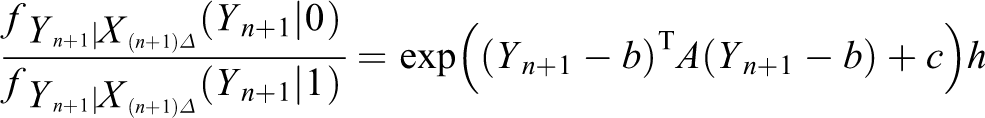
where Π₀ = P(X ₀ = 1) = 0, when n ≥ 1, the formula is as follows

$\begin{array}{l}{{\displaystyle P}}_r\left({{\displaystyle \xi }}^{}{{\displaystyle >}}_{}{{\displaystyle n\Delta +t}}_{}{{\displaystyle |}}_{}{{\displaystyle \xi }}^{}{{\displaystyle >}}_{}{{\displaystyle n\Delta }}_{},{{\displaystyle \Pi }}_n={{\displaystyle \pi }}_{}\right)={{\displaystyle P}}_{00}\left({{\displaystyle t}}_{}\right)+{{\displaystyle P}}_{01}\left({{\displaystyle t}}_{}\right)+\left({{\displaystyle P}}_{11}\left({{\displaystyle t}}_{}\right)-{{\displaystyle P}}_{00}\left({{\displaystyle t}}_{}\right)-{{\displaystyle P}}_{01}\left({{\displaystyle t}}_{}\right)\right){{\displaystyle \Pi }}_n{{\displaystyle }}_{}{{\displaystyle }}_{}{{\displaystyle }}_{}{{\displaystyle }}_{}{{\displaystyle }}_{}{{\displaystyle }}_{}{{\displaystyle }}_{}{{\displaystyle }}_{}{{\displaystyle }}_{}{{\displaystyle }}_{}{{\displaystyle }}_{}{{\displaystyle }}_{}{{\displaystyle }}_{}{{\displaystyle }}_{}{{\displaystyle }}_{}{{\displaystyle }}_{}{{\displaystyle }}_{}{{\displaystyle }}_{}={{\displaystyle R}}_{\pi }\left({{\displaystyle t}}_{}\right)\end{array}$

13

According to the above CRF, it can be concluded that the MRL function in the nth period is as follows

$\begin{array}{l}{{\displaystyle \mu }}_{n\Delta }={{\displaystyle E}}_{}\left({{\displaystyle \xi -n\Delta |\xi >n\Delta }}_{},\overrightarrow{{{\displaystyle \Pi }}_n}\right)={\displaystyle {\int }_{\text{0}}^{\infty }{{\displaystyle R}}_{}}\left({{\displaystyle t|{{\displaystyle \Pi }}_n}}_{}\right){{\displaystyle \text{d}t}}_{}\\ {{\displaystyle }}_{}{{\displaystyle }}_{}=\left(\frac{1}{{{\displaystyle \lambda }}_{12}}\right){{\displaystyle \Pi }}_n+\left(\frac{1}{{{\displaystyle \lambda }}_{01}+{{\displaystyle \lambda }}_{02}}+\frac{{{\displaystyle \lambda }}_{01}\left(\frac{1}{{{\displaystyle \lambda }}_{12}}-\frac{1}{{{\displaystyle \lambda }}_{01}+{{\displaystyle \lambda }}_{02}}\right)}{{{\displaystyle \lambda }}_{01}+{{\displaystyle \lambda }}_{02}-{{\displaystyle \lambda }}_{12}}\right)\left(1-{{\displaystyle \Pi }}_n\right)\end{array}$

14

The MRL and CRF functions have been widely used in the study of RL prediction in the field of life prediction research. Based on the formula introduced above, a real fault history data containing the binary residual observations of the study are applied thereto. To evaluate the performance of the PDP, we can estimate the MRL and CRF from the HMM. The corresponding posterior probability is calculated using the above posterior probability formula, and the results are shown in Figure 6.

Figure 6.

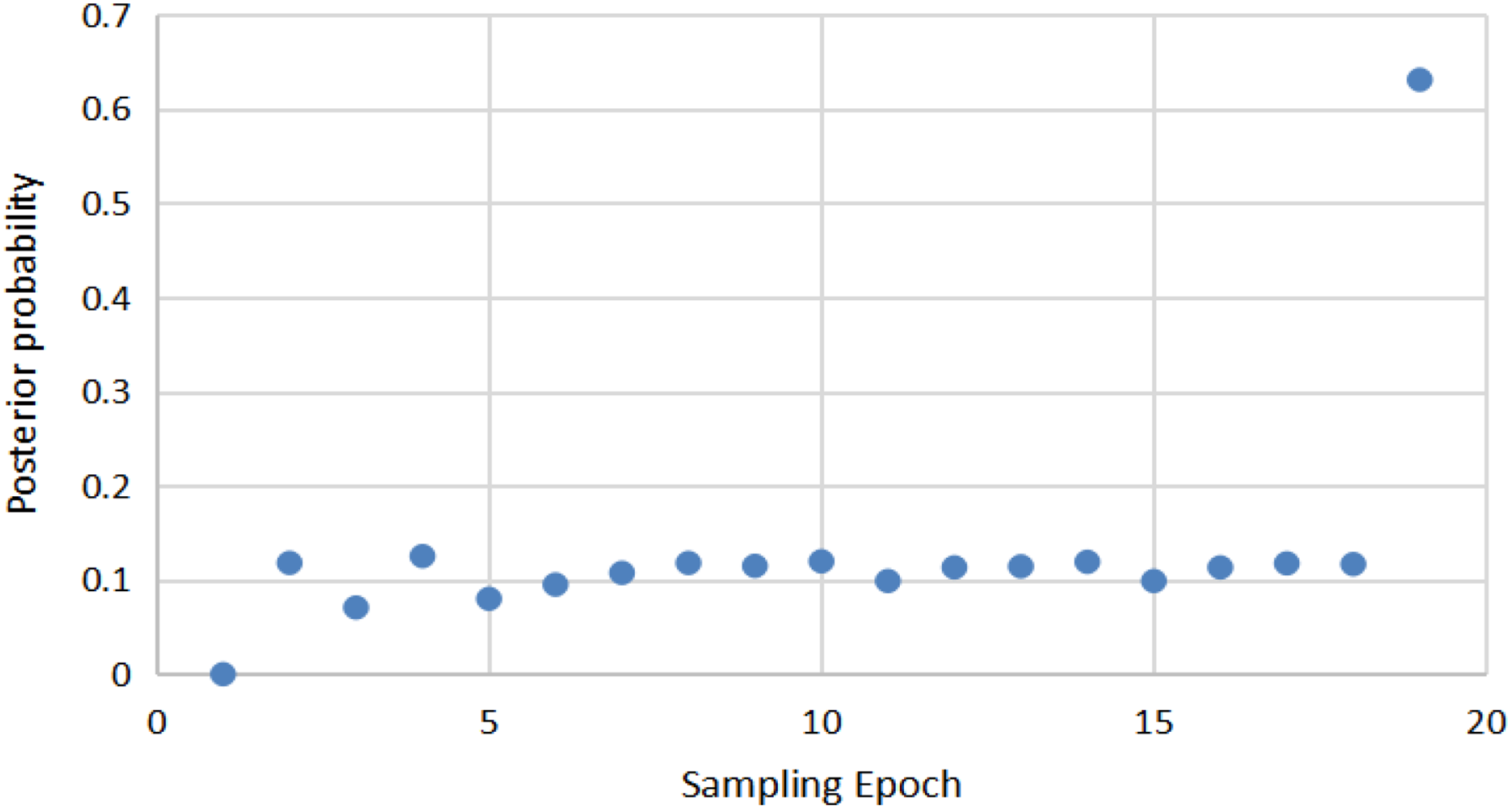
Posterior probability of the typical failure PDP. PDP: pneumatic diaphragm pump.

Figure 6 depicts the posterior probability of PDP data history. It can be seen from the figure that the PDP starts running in a healthy state and remains healthy from the first to the 18th sampling period. In the 19th sampling period, the posterior probability is significantly abrupt, indicating that the PDP entered the warning state from a healthy state, that is, from state 0 to state 1.

Based on the initial value of the posterior probability and equation (13), the estimated conditional reliability for each sampling period of PDP historical data can be derived. The result is shown in Figure 7.

Figure 7.

Conditional reliability function of failure history data.

Figure 6 shows the estimated conditional reliability for each sampling period of the PDP data history. It can be seen from the figure that reliability value of PDP from the state of health to the warning state is probably a significant downward trend in the 19th sampling period. And probably in the 26th sampling period, the system begins to enter the failure state from the warning state, indicating that the possibility of failure of PDP at this time is great. The MRL function is completely determined by the posterior probability, and the MRL of the failure historical data is shown in Figure 8. It can be seen from Figure 8 that the RL drops rapidly after the 25th sampling period, and the RL in the 26th sampling period is only 72.0559 h, indicating that PDP is close to state 2 at this time and should be comprehensive in time. Checking PDP and repairing it to avoid the progress of the production due to the fault and generate more replacement costs. Thus, the proposed model is suitable for predicting the deteriorated useful life span of a PDP.

Figure 8.

Average residual life span function of failure history data.

Conclusions

The life span of PDP in intelligent spraying is predicted according to a real multivariate diaphragm motion frequency and outlet pressure. A prediction model was developed based on MRL estimation from multivariate observations obtained from state detection of the entire system. The state follows an unobservable continuous-time hidden Markov process. The state process was modeled as a three-state continuous-time Markov chain, where the two good and warning states are unobservable, and only the fault state was observable. The VAR model was used to clean and preprocess the historical data of the healthy part and obtain the unhealthy and healthy residuals from the history data. The residual is selected as the observation process in the HMM framework. And the parameters of the HMM are estimated by means of EMA which increase considerably the speed of the computation. The RL of the PDP is predicted by deriving the explicit formula of the CRF and the MRL in the case of estimating the unknown parameters. As a result, when it is detected that the monitoring status of the PDP in the intelligent spraying system changes and the RL is greatly reduced, preventive maintenance measures should be taken immediately to ensure the entire intelligent spraying system in a healthy working state. This avoids unqualified spray products due to system failures, the delay in the entire spray line, and even the shutoff of production.

Although this article mainly analyzes the historical data of PDP in the intelligent spraying system, the methods involved in this article can be widely applied to other fields. For example, the model established in this study can be used for other types of condition monitoring data, such as quality or performance monitoring data.

In fact, the failure of PDP is a gradual process. There are numerous kinds of characteristic information throughout the life span course. However, only three states, namely the health state, the warning state, and the failure state, have been presented in this study, and the ideal results have also been obtained. This article only predicts the fault state of PDP and does not find out the reason of the malfunction. Therefore, in the future, the fault type analysis can be deeply studied.