Distributed parameter estimation in wireless sensor networks in the presence of fading channels and unknown noise variance

Abstract

Parameter estimation is one of the most important research areas in wireless sensor networks. In this study, we consider the problem of estimating a deterministic parameter over fading channels with unknown noise variance. Owing to the bandwidth constraints in wireless sensor networks, sensor observations are quantized and subsequently transmitted to the fusion center. Two types of communication channels are considered, namely, parallel-access channels and multiple-access channels. Based on the knowledge of channel statistics, the power of the received signals at the fusion center can be described by the mode of the exponential mixture distribution. The expectation maximization algorithm is used to determine maximum likelihood solutions for this mixture model. A new estimator based on the expectation maximization algorithm is subsequently proposed. Simulation results show that this estimator exhibits superior performance compared to the method of moments estimator in both parallel- and multiple-access schemes. In addition, we determine that the parallel-access scheme outperforms the multiple-access scheme when the noise variance is small and it loses its superiority when the noise variance is large.

Introduction

Wireless sensor networks (WSNs) consist of a large number of geographically distributed sensors that have limited sensing, processing, and communication capabilities. Each sensor has the ability to communicate with other sensors or a fusion center via wireless communication channels. With sensor collaboration, potentially powerful networks can be built to accomplish certain tasks, such as environment monitoring, medical care, target tracking, and military surveillance. ¹

A prevailing model used for such applications is the parallel-access channel (PAC) model wherein sensor observations are usually quantized and subsequently transmitted in parallel to the fusion center via orthogonal channels. Numerous researchers have focused on the problem of distributed estimation over PACs.^2–9 In order to estimate a deterministic parameter, the study by Ribeiro and Giannakis ² presented the maximum likelihood estimation (MLE) in Gaussian and non-Gaussian noise using a one-bit quantization scheme. Subsequently, considering the scenario wherein a total bit rate constraint was imposed, the study by Li and AlRegib ³ investigated the optimal trade-off between the number of active sensors and the quantization bit rate to minimize the estimation mean square error (MSE). Furthermore, the study by Chen and Varshney ⁴ derived the performance limit of a distributed estimation system with identical one-bit quantizers in terms of the metric minimax Cramér–Rao lower bound (CRLB). A related problem was also considered in the work by Talarico et al., ⁵ wherein a new transformed expression of the CRLB with the variance of distributed estimates was derived. The study by Sani and Vosoughi ⁶ investigated the transmission power and quantization rate allocation schemes for estimating a Gaussian vector in an inhomogeneous WSN. Moreover, considering the communication channel model of additive white Gaussian noise (AWGN), the study by Aysal and Barner ⁷ proposed the optimal maximum likelihood (ML) estimator and the suboptimal two-stage estimator. However, when the communication channel is subject to fading, the performance of these estimators will degrade severely. In the works by Wu and Cheng,^8,9 Rayleigh fading channels were included in the network model, and two parameter estimators, that is, the modified mean estimator and the liner minimum variance unbiased estimator (LMVUE), were proposed.

Recently, the problem of distributed parameter estimation over multiple-access channels (MACs) has attracted considerable attention. In the MAC scheme, multiple sensors are allowed to share a common channel, that is, communicate with the fusion center through the same MAC. Using the joint source-channel coding scheme, the study by Liu et al. ¹⁰ investigated the decentralized estimation over multiple-access fading channels and characterized the asymptotic performance of an identical source-channel mapping. In the work by Wang and Yang, ¹¹ the type-based multiple-access scheme was proposed. In this scheme, each sensor communicates with the fusion center over a dedicated channel that corresponds to its observation type. In the work by Venkategowda et al., ¹² pre-coding techniques were introduced into the parameter estimation over coherent MACs and a robust distributed estimator was derived to minimize the worst-case error.

In the aforementioned papers, the knowledge of channel noise is usually assumed to be available at the fusion center. Although the channel noise can be estimated in advance, sensors might be required to expend much effort and hence it results in significant overhead. Hence, it is necessary to further study the estimation fusion issues with unknown noise statistics.

Regarding the problem of parameter estimation in WSNs, the conventional MLE method can obtain the estimates with desirable properties. Unfortunately, it does not have a closed-form solution in general. Although the MLE can be determined using either the Newton–Raphson or the Nelder–Mead algorithm, ¹³ the expectation maximization (EM) method ¹⁴ provides an estimator that is easy to determine and simple to implement. It has a broad range of applications, including environment monitoring, image segmentation, object tracking, modulation classification, and so on.^15–21

In our study, considering one-bit quantization at local sensors and fading channels with unknown noise variance, we use the EM algorithm to determine the ML estimates of unknown parameters.

The remainder of the article is organized as follows. In section “Problem formulation,” we formulate the estimation fusion issues in the PAC and MAC schemes. In sections “MLE over parallel channels” and “MLE over MACs,” the EM approach for the MLE of unknown parameters is derived. In section “Threshold design,” the problem of designing the quantization threshold is investigated. The performance of the EM estimator is demonstrated in section “Performance evaluation.” Finally, we present concluding remarks in section “Conclusion.”

Problem formulation

We consider the problem of estimating a deterministic parameter $\theta$ over fading channels in WSNs. It is assumed that N sensors collect observations, which are corrupted by noise. The sensor observation $x_j$ is given as follows

$$x_j=\theta +n_{j}j=1,2,\dots ,N$$

(1)

where $n_j(j=1,\dots ,N)$ are zero-mean additive Gaussian noises with variance ${\sigma }_n^2$ . Owing to bandwidth constraints, the observation $x_j$ is generally quantized before communication. Furthermore, we adopt the following quantization scheme

$$b_j=\{\begin{array}{cc}1\hfill & x_j\ge \tau \hfill \\ \multicolumn{1}{c}{0}& x_j<\tau \hfill \end{array}$$

(2)

where $\tau$ is a quantization threshold. Thus, $b_j$ is a Bernoulli random variable with the following parameter

$$Pr\{b_j=1\}=F(\theta )$$

(3)

where

$$F(\theta )=\underset{\tau }{\overset{\infty }{\int }}\frac{1}{\sqrt{2\pi }{\sigma }_n}{e}^{-\frac{{(x-\theta )}^2}{2{\sigma }_n^2}}\mathrm{dx}$$

(4)

Based on the above quantization scheme, sensor j may transmit only one bit per $b_j$ to the fusion center through wireless channels. In this section, we consider two types of channel structures, namely, PACs and MACs.

PACs

Figure 1(a) depicts a typical PAC structure wherein local sensors communicate with the fusion center via orthogonal channels. We assume that the PACs undergo independent fading and the channel noise is uncorrelated from channel to channel. Since most WSNs operate at short range and low bit rate owing to energy and bandwidth limitations, we further assume flat fading channels between the local sensors and the fusion center. Thus, the received data at the fusion center can be expressed as follows

$$y_j=h_j{e}^{i{\varphi }_j}{b}_j+v_j,j=1,\dots ,N$$

(5)

where $h_j$ and ${\varphi }_j$ are the fading envelope and phase, respectively, and $v_j$ is a zero-mean complex Gaussian noise whose real and imaginary parts have equal variance ${\sigma }_v^2$ ( ${\sigma }_v$ is unknown at the fusion center).

Figure 1.

System model: (a) PAC and (b) MAC.

Using the data received from all the sensors, the fusion center obtains the estimate of the unknown parameter θ. In order to simplify, we adopt the incoherent reception at the fusion center and develop the parameter estimator based on the power of the received signals. The signal power of the jth channel output is denoted by $z_j(z_j=|y_j{|}^2)$ . Assuming a Rayleigh fading channel with unit power, the probability density function (PDF) of $h_j$ is

$$p(h_j)=2h_j{e}^{-h_j^2}$$

(6)

Given $p(h_j)$ , the conditional PDF of $z_j$ can be obtained as follows ²²

$$p(z_j|b_j=0)=\frac{1}{2{\sigma }_v^2}{e}^{-\frac{z_j}{2{\sigma }_v^2}}$$

(7)

$$p(z_j|b_j=1)=\frac{1}{1+2{\sigma }_v^2}{e}^{-\frac{z_j}{1+2{\sigma }_v^2}}$$

(8)

Thus, the likelihood of $z_j$ can be calculated as follows

$$p(z_j;\theta )=\left[1-F(\theta )\right]p\left(z_j|b_j=0\right)+F(\theta )p\left(z_j|b_j=1\right)$$

(9)

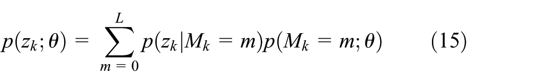
Let us set $p(z_j;{\lambda }_1)$ and $p(z_j;{\lambda }_2)$ as two generic exponential distributions corresponding to the parameters ${\lambda }_1=1/(2{\sigma }_v^2)$ and ${\lambda }_2=1/(1+2{\sigma }_v^2)$ , respectively. Hence, $z_j$ can be modeled as the following exponential mixture distribution

$$p(z_j;\theta )=[1-F(\theta )]p(z_j;{\lambda }_1)+F(\theta )p(z_j;{\lambda }_2)$$

(10)

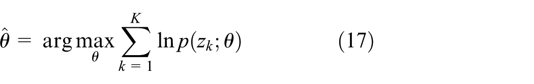
The MLE of θ can be determined straightforwardly by maximizing the likelihood function over θ

$${\hat{\theta }}_{\mathrm{ML}}=\arg \underset{\theta }{max}{\mathrm{\Pi }}_{j=1}^{N}p(z_j;\theta )$$

(11)

MACs

As shown in Figure 1(b), N sensors are uniformly partitioned into K groups, each group containing $L=N/K$ sensors. Using the MAC scheme, each group is allocated a separate channel, and sensors in each group can transmit simultaneously over the same channel. Hence, the communication bandwidth is greatly reduced compared to the case of requiring N orthogonal channels.

At the fusion center, the received signal can be expressed as follows

$$y_k=\sum _{l=1}^L{h}_{k,l}{e}^{i{\varphi }_{k,l}}{b}_{k,l}+v_k,k=1,\dots ,K$$

(12)

Furthermore, we denote the received signal power as $z_k$ and consider non-coherent reception at the fusion center. A random variable $M_k=\sum _{l=1}^L{b}_{k,l}$ (i.e. the total number of sensors that decide to transmit) is defined, and it is assumed that the sequence $M=\{M_k,k=1,\dots ,K\}$ is independent and identically distributed. This assumption is reasonable because the observations of local sensors are normally independent of each other across sensors, and an identical quantization threshold is applied to all the sensors. Thus, we have

$$p(M_k=m;\theta )=\left(\begin{array}{c}L\hfill \\ \multicolumn{1}{c}{m}\end{array}\right){(F(\theta ))}^m{(1-F(\theta ))}^{L-m}$$

(13)

Under the assumption of a Rayleigh fading channel with unit power, we obtain

$$p\left(z_k|M_k=m\right)=\frac{1}{m+2{\sigma }_v^2}{e}^{-\frac{z_k}{m+2{\sigma }_v^2}}$$

(14)

Subsequently, the distribution of $z_k$ can be expressed as follows

$$p(z_k;\theta )=\sum _{m=0}^{L}p\left(z_k|M_k=m\right)p(M_k=m;\theta )$$

(15)

Substituting equations (13) and (14) into equation (15), we obtain

$$p(z_k;\theta )=\sum _{m=0}^L\left(\begin{array}{c}L\hfill \\ \multicolumn{1}{c}{m}\end{array}\right)\frac{{(F(\theta ))}^m{(1-F(\theta ))}^{L-m}}{m+2{\sigma }_v^2}{e}^{-\frac{z_k}{m+2{\sigma }_v^2}}$$

(16)

With the received signal from all the groups, the ML estimate of the parameter θ is subsequently obtained as follows

$$\hat{\theta }=\arg \underset{\theta }{max}\sum _{k=1}^K\ln p(z_k;\theta )$$

(17)

MLE over parallel channels

Given the quantization threshold $\tau$ , there is a one-to-one mapping between $\theta$ and $F(\theta )$ , as shown in Figure 2. Once the MLE of $\theta$ is available, we can determine the MLE of $F(\theta )$ using the invariance of MLE. Therefore, in order to simplify, we examine the estimation of $F(\theta )$ instead of θ. The MLE for $F(\theta )$ is expressed as follows

$$\begin{array}{c}\multicolumn{1}{c}{\hat{F}{\left(\theta \right)}_{\mathrm{ML}}=\arg \underset{F\left(\theta \right)}{max}\sum _{j=1}^N\ln p(z_j;F\left(\theta \right),{\sigma }_v)}\\ =\arg \underset{F(\theta )}{max}\sum _{j=1}^N\ln \hfill \\ \multicolumn{1}{c}{\{[1-F\left(\theta \right)]p(z_j;{\lambda }_1\left({\sigma }_v\right))+F\left(\theta \right)p(z_j;{\lambda }_2\left({\sigma }_v\right))\}.}\end{array}$$

(18)

Figure 2.

The curves of $F(\theta )$ as a function of $\theta$ for different $\tau$ $({\sigma }_n=1)$ .

EM for parameter estimation over parallel channels

Since there is no closed-form solution to equation (18), we consider the MLE using the EM algorithm. The EM algorithm is an elegant and powerful method to determine ML solutions for models with latent variables. It is an iterative algorithm which alternates between inferring the missing values given the parameters (E step), and then optimizing the parameters given the “filled-in” data (M step). It can approximately achieve the performance of the MLE with low computational complexity, ¹⁴ which renders it suitable for resource-constrained WSNs.

The formulation of the mixture problem in the EM framework is achieved by augmenting the observed data vector $\mathbf{z}=\{z_j{\}}_{j=1}^N$ with the associated component-label vector $\mathbf{\gamma }=\{{\gamma }_j{\}}_{j=1}^N$ . Each ${\gamma }_j$ assumes a value from the set $\{0,1\}$ , where ${\gamma }_j=0$ indicates that $z_j$ is generated from the distribution $p(z_j;{\lambda }_1)$ , whereas ${\gamma }_j=1$ indicates that $z_j$ is generated from the distribution $p(z_j;{\lambda }_2)$ .

The unknown parameter set is denoted as $\mathbf{\xi }=\{F(\theta ),{\sigma }_v\}$ . The complete data log-likelihood is subsequently expressed as follows

$$\begin{array}{c}\ln p(\mathbf{z}\mathbf{,}\mathbf{\gamma }\mathbf{;}\mathbf{\xi }\mathbf{)}\hfill \\ =\sum _{j=1}^N\{(1-{\gamma }_j)\ln [(1-F(\theta ))p(z_j;{\lambda }_1({\sigma }_v))]\hfill \\ \multicolumn{1}{c}{+{\gamma }_j\ln [F(\theta )p(z_j;{\lambda }_2({\sigma }_v))]\}}\end{array}$$

(19)

The ML estimator based on the EM algorithm (EMML) is described by the following steps:

1. An initial setting is chosen for the parameters ${{\hat{\sigma }}^0}_v$ and $\hat{F}(\theta {)}^0$ .

2. E step—Given the observation z and current parameter set $\widehat{{\mathbf{\xi }}^t}$ , the conditional expectation of joint distribution $p(\mathbf{z},\mathbf{\gamma }\mathbf{;}\mathbf{\xi }\mathbf{)}$ is computed as follows

$$\begin{array}{l}Q\left(\mathbf{\xi },{\widehat{\mathbf{\xi }}}^t\right)=E\left[\ln p\left(\mathbf{z},\mathbf{\gamma };\mathbf{\xi }\right)|\mathbf{z};{\widehat{\mathbf{\xi }}}^t\right]\\ =\sum _{j=1}^N\left\{\left(1-w_j^{t+1}\right)\ln \left[\left(1-F\left(\theta \right)\right)p\left(z_j;{\lambda }_1\left({\sigma }_v\right)\right)\right]+w_j^{t+1}\ln \left[F\left(\theta \right)p\left(z_j;{\lambda }_2\left({\sigma }_v\right)\right)\right]\right\}\end{array}$$

(20)

where

$$w_j^{t+1}=\frac{\hat{F}{\left(\theta \right)}^{t}p(z_j;{\lambda }_2\left({\hat{\sigma }}_v^t\right))}{[1-\hat{F}{\left(\theta \right)}^t]p(z_j;{\lambda }_1\left({\hat{\sigma }}_v^t\right))+\hat{F}{\left(\theta \right)}^{t}p(z_j;{\lambda }_2\left({\hat{\sigma }}_v^t\right))}$$

(21)

• 3. M step—The parameter set is updated by maximizing this function

$$\widehat{{\mathbf{\xi }}^{t+1}}=\arg \underset{\mathbf{\xi }}{max}Q(\mathbf{\xi }\mathbf{,}\widehat{{\mathbf{\xi }}^{\mathbf{t}}})$$

(22)

We rewrite $Q(\mathbf{\xi }\mathbf{,}\widehat{{\mathbf{\xi }}^{\mathbf{t}}}\mathbf{)}$ as follows

$$\begin{array}{c}\multicolumn{1}{c}{Q(\mathbf{\xi }\mathbf{,}{\hat{\mathbf{\xi }}}^{\mathbf{t}}\mathbf{)}\mathbf{=}\sum _{j=1}^N\{(1-w_j^{t+1})\ln \left[\frac{1-F(\theta )}{2{\sigma }_v^2}{e}^{-\frac{z_j}{2{\sigma }_v^2}}\right]}\\ \multicolumn{1}{c}{+w_j^{t+1}\ln \left[\frac{F\left(\theta \right)}{1+2{\sigma }_v^2}{e}^{-\frac{z_j}{1+2{\sigma }_v^2}}\right]\}}\end{array}$$

(23)

Differentiating with respect to $F(\theta )$ and ${\sigma }_v$ , and setting the result to zero, we obtain

$$\hat{F}{\left(\theta \right)}^{t+1}=\frac{\sum _{j=1}^N{w}_j^{t+1}}{N}$$

(24)

and ${\hat{\sigma }}_v^{t+1}$ , which satisfies the following equation

$$x^6+a_1{x}^4+a_2{x}^2+a_3=0$$

(25)

where

$$a_1=\frac{1}{2N}\sum _{j=1}^N(2-w_j^{t+1}-z_j)$$

(26)

$$a_2=\frac{1}{4N}\sum _{j=1}^N(1-w_j^{t+1})(1-2z_j)$$

(27)

$$a_3=\frac{1}{8N}\sum _{j=1}^N(w_j^{t+1}-1)z_j$$

(28)

In order to solve equation (25), it is necessary to begin with a definition. Thus, we define $X=x^2+(a_1/3)$ and rewrite equation (25) as follows

$$X^3+\mathrm{pX}+q=0$$

(29)

where

$$p=-\frac{1}{3}{a}_1^2+a_2$$

(30)

$$q=\frac{2}{27}{a}_1^3-\frac{1}{3}{a}_1{a}_2+a_3$$

(31)

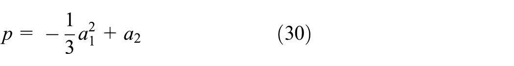
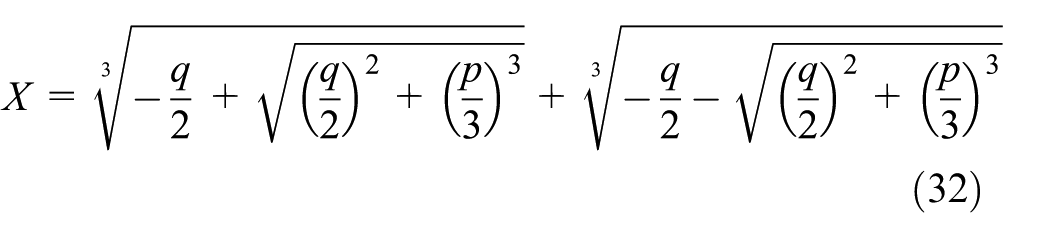
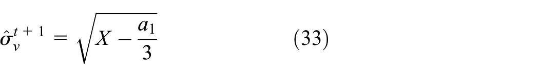
Using the standard method generally known as Cardan’s solution, ²³ we obtain three roots of equation (29). Rounding the two complex roots, we obtain

$$X=\sqrt[3]{-\frac{q}{2}+\sqrt{{\left(\frac{q}{2}\right)}^2+{\left(\frac{p}{3}\right)}^3}}+\sqrt[3]{-\frac{q}{2}-\sqrt{{\left(\frac{q}{2}\right)}^2+{\left(\frac{p}{3}\right)}^3}}$$

(32)

Using the above result, we obtain

$${\hat{\sigma }}_v^{t+1}=\sqrt{X-\frac{a_1}{3}}$$

(33)

• 4. The convergence of the parameter is verified. Given a sufficiently small value $\epsilon$ , if the difference between successive parameter estimates is less than $\epsilon$ (i.e. $|\hat{F}(\theta {)}^{t+1}-\hat{F}(\theta {)}^t|<\epsilon$ ), the iteration ends. Otherwise, if the convergence criterion is not satisfied, we return to step 2 and set t = t + 1.

Setting initial values

A suitable initialization is important for the EM algorithm to converge to the global maximum. In this section, we propose a moment-based approach to obtain the initial values of ${\hat{\sigma }}_v$ and $\hat{F}(\theta )$ .

The mean and variance of $z_j$ can be calculated as follows

$$E[z_j]=2{\sigma }_v^2+F(\theta )$$

(34)

$$\mathrm{Var}[z_j]=4{\sigma }_v^4+(2+4{\sigma }_v^2)F(\theta )-F(\theta {)}^2$$

(35)

Using equations (34) and (35), we obtain a second-order polynomial in $F(\theta )$

$$2F(\theta {)}^2-2F(\theta )+\mathrm{Var}(z_j)-E^2(z_j)=0$$

(36)

Since $\mathrm{Var}(z_j)-E^2(z_j)=2F(\theta )[1-F(\theta )]\le 1/2$ , the roots of equation (36) are obtained as follows

$$F(\theta )=\{\begin{array}{c}\frac{1}{2}\{1-\sqrt{1-2[\mathrm{Var}(z_j)-E^2(z_j)]}\}\mathrm{if}F(\theta )\le 0.5\hfill \\ \multicolumn{1}{c}{\frac{1}{2}\{1+\sqrt{1-2[\mathrm{Var}(z_j)-E^2(z_j)]}\}\mathrm{if}F(\theta )>0.5}\end{array}$$

(37)

In the case of a large number of observations, using the normal approximation, we obtain the initial value of $\hat{F}(\theta )$

$$\hat{F}(\theta )=\{\begin{array}{c}\frac{1}{2}\{1-\sqrt{1-2[\frac{1}{N-1}\sum _{j=1}^N{(z_j-\frac{1}{N}\sum _{j=1}^N{z}_j)}^2-{\left(\frac{1}{N}\sum _{j=1}^N{z}_j\right)}^2]}\}\mathrm{if}F(\theta )\le 0.5\hfill \\ \multicolumn{1}{c}{\frac{1}{2}\{1+\sqrt{1-2[\frac{1}{N-1}\sum _{j=1}^N{(z_j-\frac{1}{N}\sum _{j=1}^N{z}_j)}^2-{\left(\frac{1}{N}\sum _{j=1}^N{z}_j\right)}^2]}\}\mathrm{if}F(\theta )>0.5}\end{array}$$

(38)

Substituting $\hat{F}(\theta )$ into equation (34), we thus obtain the initial value of ${\hat{\sigma }}_v$

$${\hat{\sigma }}_v=\sqrt{\frac{1}{2}[\frac{1}{N}\sum _{j=1}^N{z}_j-\hat{F}(\theta )]}$$

(39)

CRLB

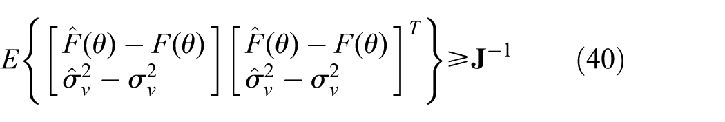
The performance measure of interest is the MSE of the estimates. It is well known that the CRLB, a classical result, provides the lower bound of the MSE for any unbiased estimator. This implies that the theoretical CRLB is a reliable performance predictor. The CRLB of $\mathbf{\xi }$ can be obtained as follows

$$E\left\{\left[\begin{array}{c}\hat{F}(\theta )-F(\theta )\hfill \\ \multicolumn{1}{c}{{\hat{\sigma }}_v^2-{\sigma }_v^2}\end{array}\right]{\left[\begin{array}{c}\hat{F}(\theta )-F(\theta )\hfill \\ \multicolumn{1}{c}{{\hat{\sigma }}_v^2-{\sigma }_v^2}\end{array}\right]}^T\right\}\ge {\mathbf{J}}^{-1}$$

(40)

where J is the Fisher information matrix (FIM) and its elements are expressed as follows

$$J_{11}=\sum _{j=1}^N\underset{-\infty }{\overset{\infty }{\int }}\left\{\frac{1}{p(z_j;F(\theta ),{\sigma }_v^2)}{\left[\frac{\partial p(z_j;F(\theta ),{\sigma }_v^2)}{\partial F(\theta )}\right]}^2\right\}d{z}_j$$

(41)

$$J_{22}=\sum _{j=1}^N\underset{-\infty }{\overset{\infty }{\int }}\left\{\frac{1}{p(z_j;F(\theta ),{\sigma }_v^2)}{\left[\frac{\partial p(z_j;F(\theta ),{\sigma }_v^2)}{\partial {\sigma }_v^2}\right]}^2\right\}d{z}_j$$

(42)

$$\begin{array}{l}{J}_{12}=J_{21}\\ =\sum _{j=1}^N\underset{-\infty }{\overset{\infty }{\int }}\left\{\frac{1}{p\left(z_j;F(\theta ),{\sigma }_v^2\right)}\left[\frac{\partial p\left(z_j;F(\theta ),{\sigma }_v^2\right)}{\partial F(\theta )}\cdot \frac{\partial p\left(z_j;F(\theta ),{\sigma }_v^2\right)}{\partial {\sigma }_v^2}\right]\right\}d{z}_j\end{array}$$

(43)

where

$$\frac{\partial p(z_j;F(\theta ),{\sigma }_v^2)}{\partial F(\theta )}=-\frac{1}{2{\sigma }_v^2}{e}^{-\frac{z_j}{2{\sigma }_v^2}}+\frac{1}{1+2{\sigma }_v^2}{e}^{-\frac{z_j}{1+2{\sigma }_v^2}}$$

(44)

$$\begin{array}{c}\multicolumn{1}{c}{\frac{\partial p(z_j;F(\theta ),{\sigma }_v^2)}{\partial {\sigma }_v^2}=[1-F(\theta )]\frac{z_j-2{\sigma }_v^2}{4{\sigma }_v^6}{e}^{-\frac{z_j}{2{\sigma }_v^2}}}\\ \multicolumn{1}{c}{+F(\theta )\frac{2z_j-2-4{\sigma }_v^2}{{(1+2{\sigma }_v^2)}^3}{e}^{-\frac{z_j}{1+2{\sigma }_v^2}}}\end{array}$$

(45)

MLE over MACs

EMML estimator over MACs

The ML estimator of the parameter set $\mathbf{\xi }$ is expressed as follows

$$\begin{array}{c}\multicolumn{1}{c}{\hat{\mathbf{\xi }}=\arg \underset{\mathbf{\xi }}{max}\sum _{k=1}^K\ln p(z_k;\mathbf{\xi })}\\ \multicolumn{1}{c}{=\arg \underset{\mathbf{\xi }}{max}\sum _{k=1}^K}\\ \multicolumn{1}{c}{\ln \left\{\sum _{m=0}^L\left(\begin{array}{c}L\hfill \\ \multicolumn{1}{c}{m}\end{array}\right)\frac{{(F(\theta ))}^m{(1-F(\theta ))}^{L-m}}{m+2{\sigma }_v^2}{e}^{-\frac{z_k}{m+2{\sigma }_v^2}}\right\}}\end{array}$$

(46)

Since the maximization of the logarithm likelihood function in equation (46) entails high computational complexity, we use the EM algorithm to implement the MLE of $\mathbf{\xi }$ . Given a current estimate $\widehat{{\mathbf{\xi }}^t}$ , the iterative equation is expressed as follows

$$\begin{array}{c}{\widehat{\mathbf{\xi }}}^{t+1}=\arg \underset{\xi }{\max }E\left[\ln p\left(\mathbf{z},\mathbf{M};\mathbf{\xi }\right)|\mathbf{z};{\widehat{\mathbf{\xi }}}^t\right]\\ =\arg \underset{\mathbf{\xi }}{\max }\sum _{\mathbf{M}}\ln p\left(\mathbf{z},\mathbf{M};\mathbf{\xi }\right)p\left(\mathbf{M}|\mathbf{z};{\widehat{\mathbf{\xi }}}^t\right)\end{array}$$

(47)

Thus, we obtain

$$\begin{array}{c}\widehat{F}{(\theta )}^{t+1}=\arg \underset{F(\theta )}{\max }\sum _{\mathbf{M}}\ln p\left(\mathbf{M};F(\theta )\right)p\left(\mathbf{M}|\mathbf{z};{\widehat{\mathbf{\xi }}}^t\right)\\ =\arg \underset{F(\theta )}{\max }\sum _{k=1}^K\sum _{m=0}^L\ln p\left(M_k=m;F(\theta )\right)p\left(M_k=m|z_k;{\widehat{\xi }}^t\right)\end{array}$$

(48)

and

$$\begin{array}{c}{\widehat{\sigma }}_v^{t+1}=\arg \underset{{\sigma }_v}{\max }\sum _M\ln p\left(z|M;{\sigma }_v\right)p\left(M|z;{\widehat{\xi }}^t\right)\\ =\arg \underset{{\sigma }_v}{\max }\sum _{k=1}^K\sum _{m=0}^L\ln p\left(z_k|M_k=m;{\sigma }_v\right)p\left(M_k=m|z_k;{\widehat{\xi }}^t\right)\end{array}$$

(49)

Substituting equations (13) and (14) into equations (48) and (49), respectively, differentiating with respect to $F(\theta )$ and ${\sigma }_v$ and setting the result to zero yield

$$\hat{F}{\left(\theta \right)}^{t+1}=\frac{\sum _{k=1}^K\sum _{m=0}^{L}p(M_k=m|z_k;{\hat{\mathbf{\xi }}}^t)m}{N}$$

(50)

and

$$\sum _{k=1}^K\sum _{m=0}^L\frac{p(M_k=m|z_k;{\hat{\mathbf{\xi }}}^t)(z_k-m-2{\left({\hat{\sigma }}_v^{t+1}\right)}^2)}{{(m+2{\left({\hat{\sigma }}_v^{t+1}\right)}^2)}^2}=0$$

(51)

Using Bayes’ rule, we obtain

$$\begin{array}{c}\multicolumn{1}{c}{p(M_k=m|z_k;{\hat{\mathbf{\xi }}}^t)=\frac{p\left(z_k|M_k=m;{\hat{\mathbf{\xi }}}^t\right)p(M_k=m;{\hat{\mathbf{\xi }}}^t)}{p(z_k;{\hat{\mathbf{\xi }}}^t)}}\\ \multicolumn{1}{c}{=\frac{\left(\begin{array}{c}L\hfill \\ \multicolumn{1}{c}{m}\end{array}\right)\frac{{\left(\hat{F}{(\theta )}^t\right)}^m{(1-\hat{F}{(\theta )}^t)}^{L-m}}{m+2{({\hat{\sigma }}_v^t)}^2}{e}^{-\frac{z_k}{m+2{({\hat{\sigma }}_v^t)}^2}}}{\sum _{m=0}^L\left(\begin{array}{c}L\hfill \\ \multicolumn{1}{c}{m}\end{array}\right)\frac{{\left(\hat{F}{(\theta )}^t\right)}^m{(1-\hat{F}{(\theta )}^t)}^{L-m}}{m+2{({\hat{\sigma }}_v^t)}^2}{e}^{-\frac{z_k}{m+2{({\hat{\sigma }}_v^t)}^2}}}}\end{array}$$

(52)

Since a closed-form expression of ${\hat{\sigma }}_v^{t+1}$ is not directly possible from equation (51), the Newton–Raphson method is used to determine its numerical solution. Equations (50)–(52) formulate the iterative EM steps for the estimation of the parameter set $\mathbf{\xi }$ . The iterations are started using the initial setting of $\widehat{{\mathbf{\xi }}^0}$ and stopped when the predefined convergence criterion is satisfied.

Setting initial values

The moment-based approach is used to derive the initial values of $\hat{F}(\theta )$ and ${\hat{\sigma }}_v$ . Owing to the independence assumptions described in section “Problem formulation,” the mean and variance of $z_k$ can be expressed as follows

$$E[z_k]=\mathrm{LF}(\theta )+2{\sigma }_v^2$$

(53)

$$\mathrm{Var}[z_k]=L(L-2)F(\theta {)}^2+(2+4{\sigma }_v^2)\mathrm{LF}(\theta )+4{\sigma }_v^4$$

(54)

Given these statistics, we can calculate the initial values of $\hat{F}(\theta )$ and ${\hat{\sigma }}_v$ following a similar procedure as equations (36)–(39). Thus, we obtain

$$\hat{F}(\theta )=\{\begin{array}{c}\frac{1}{2}\{1-\sqrt{1-\frac{2}{L}[\frac{1}{K-1}\sum _{k=1}^K{(z_k-\frac{1}{K}\sum _{k=1}^K{z}_k)}^2-{\left(\frac{1}{K}\sum _{k=1}^K{z}_k\right)}^2]}\}\mathrm{if}F(\theta )\le 0.5\hfill \\ \multicolumn{1}{c}{\frac{1}{2}\{1+\sqrt{1-\frac{2}{L}[\frac{1}{K-1}\sum _{k=1}^K{(z_k-\frac{1}{K}\sum _{k=1}^K{z}_k)}^2-{\left(\frac{1}{K}\sum _{k=1}^K{z}_k\right)}^2]}\}\mathrm{if}F(\theta )>0.5}\end{array}$$

(55)

and

$${\hat{\sigma }}_v=\sqrt{\frac{1}{2}[\frac{1}{K}\sum _{k=1}^K{z}_k-L\hat{F}(\theta )]}$$

(56)

CRLB

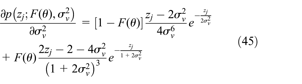
In order to determine the CRLB, we first derive the FIM. Differentiating the likelihood function $p(z_k;F(\theta ),{\sigma }_v^2)$ , we have

$$\begin{array}{c}\frac{\partial p(z_k;F(\theta ),{\sigma }_v^2)}{\partial F(\theta )}\hfill \\ =\sum _{m=0}^L\left(\begin{array}{c}L\hfill \\ \multicolumn{1}{c}{m}\end{array}\right)\frac{{(F(\theta ))}^{m-1}{(1-F(\theta ))}^{L-m-1}(m-\mathrm{LF}(\theta ))}{m+2{\sigma }_v^2}{e}^{-\frac{z_k}{m+2{\sigma }_v^2}}\hfill \end{array}$$

(57)

and

$$\begin{array}{c}\frac{\partial p(z_k;F(\theta ),{\sigma }_v^2)}{\partial {\sigma }_v^2}\hfill \\ =\sum _{m=0}^L\left(\begin{array}{c}L\hfill \\ \multicolumn{1}{c}{m}\end{array}\right)\frac{2{(F(\theta ))}^m{(1-F(\theta ))}^{L-m}(z_k-m-2{\sigma }_v^2)}{{(m+2{\sigma }_v^2)}^3}\hfill \\ \multicolumn{1}{c}{e^{-\frac{z_k}{m+2{\sigma }_v^2}}}\end{array}$$

(58)

Similar to section “CRLB,” substituting equations (57) and (58) into equations (41)–(43), with j and N replaced by k and K, respectively, we obtain the elements of the FIM. Finally, using equation (40), we obtain the CRLB.

Threshold design

In this section, the problem of designing the quantization threshold is analyzed. The CRLB is adopted as a criterion to set the threshold optimally.

Let $\hat{\theta }$ be the MLE of the unknown parameter $\theta$ . Under the assumption of some regularity conditions, ²⁴ the estimate $\hat{\theta }$ is asymptotically distributed according to

$$\hat{\theta }{~}^{a}N(\theta ,B(\theta ;\tau ,{\sigma }_v))$$

(59)

where $B(\theta ;\tau ,{\sigma }_v)$ is the CRLB for $\theta$

$$B(\theta ;\tau ,{\sigma }_v)=\frac{{[{\mathbf{J}}^{-1}(\mathbf{\xi }\mathbf{)}\mathbf{]}}_{11}}{{\left(\frac{\partial F(\theta ;\tau )}{\partial \theta }\right)}^2}$$

(60)

In other words, the ML estimate is asymptotically unbiased and asymptotically attains the CRLB.

Since the CRLB is a good performance metric for the MLE, a threshold that minimizes the CRLB is optimal with an ML fusion center. Figure 3 depicts the CRLB for $\theta$ in the PAC and MAC schemes, in which there obviously exists an optimal threshold corresponding to the minimum CRLB. From equation (60), $B(\theta ;\tau ,{\sigma }_v)$ depends on $\theta$ and ${\sigma }_v$ . Without $\theta$ and ${\sigma }_v$ a priori, it is impossible to obtain this optimal threshold. Furthermore, the CRLB is a function of $\theta$ . In general, there does not exist one threshold that can minimize the CRLB for all $\theta$ . To ensure accurate estimation over the entire parameter range, here we adopt the minimax criterion, ⁴ that is, we try to minimize the worst-case CRLB among all $\theta$ .

Figure 3.

CRLB for $\theta$ as a function of the threshold $\tau$ ( $\theta =1$ , ${\sigma }_n=1$ , N = 300, and L = 3).

In many practical applications, the dynamic range of $\theta$ is often assumed to be known, such that $\theta$ lies in $(0,\Delta )$ , where $\Delta$ is a known constant. Define the worst-case CRLB as follows

$$C_w(\tau )=\underset{\theta }{max}B(\theta ;\tau ,{\sigma }_v)$$

(61)

The optimal threshold is then the solution of the following optimization problem

$${\tau }_{\mathrm{opt}}=\arg \underset{\tau }{min}{C}_w(\tau )$$

(62)

Since ${\sigma }_v$ is unknown, there is not much that we can do to set $\tau$ optimally. However, from Figure 4, we can observe that the optimum threshold is insensitive to variations of the channel signal-to-noise ratio (SNR, $\mathrm{SNR}:10{\log }_{10}(1/(2{\sigma }_v^2))$ dB). When SNR varies from 0 to 20 dB, the optimal threshold ${\tau }_{\mathrm{opt}}$ moves from $1.43{\sigma }_n$ to $0.59{\sigma }_n$ for the PAC scheme, and it moves from $1.54{\sigma }_n$ to $0.96{\sigma }_n$ for the MAC scheme. It implies that we can find an approximately optimal threshold by replacing ${\sigma }_v$ with its initial estimate. Thus, the optimization problem equation (62) can be relaxed to obtain

$${\tau }_{\mathrm{app}}=\arg \underset{\tau }{min}\underset{\theta }{max}B(\theta ;\tau ,{\hat{\sigma }}_v)$$

(63)

Figure 4.

Variation of the optimal threshold with the SNR ( $\Delta /{\sigma }_n=1$ and L = 2).

Note that the estimation performance of ${\sigma }_v$ also depends on the selection of the initial quantization threshold ${\tau }^0$ . Figure 5 depicts the CRLB for ${\sigma }_v$ using different quantization thresholds. As shown, the estimation performance of ${\sigma }_v$ can improve significantly when the quantization threshold is sufficiently larger than the true parameter $\theta$ . To ensure accurate estimation of ${\sigma }_v$ , we should choose a large value of ${\tau }^0$ within the inherent dynamic range limitation of the signal quantizer. Using this threshold, each local sensor quantizes its observation to one bit and sends it to the fusion center. With the received data from all the sensors, the fusion center estimates ${\sigma }_v$ using the EM method. Straightforwardly, the approximately optimal threshold in equation (63) is obtained.

Figure 5.

CRLB for ${\sigma }_v$ as a function of $\tau$ ( $\theta =1$ , ${\sigma }_n=1$ , SNR = 5 dB, N = 300, and L = 3).

Performance evaluation

In this section, Monte Carlo simulations are performed to evaluate the performance of the EMML estimator. The EM algorithm is stopped when the difference between successive parameter estimates is less than ${10}^{-6}$ .

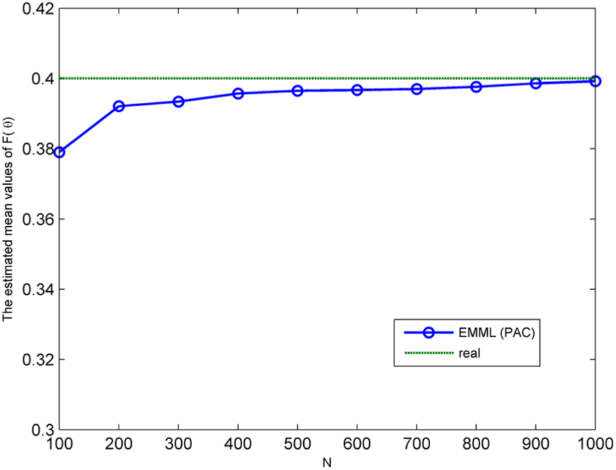
First, we consider the scenario of parallel channels. Without loss of generality, the value of $F(\theta )$ is set to 0.4 (unless otherwise specified). Numerical results are obtained by averaging over 1000 experiments. Figure 6 shows the sample means of $F(\theta )$ as a function of the number of sensors. The channel SNR is set to 5 dB. When the number of sensors is relatively small, the EMML estimator is biased. Otherwise, as this number increases, the estimator becomes asymptotically unbiased. In order to evaluate the performance of the EMML estimator, we subsequently compare it with the method of moments estimator (MME) and the LMVUE described in the work by Wu and Cheng. ⁹ Figure 7 shows the estimation performance in terms of MSE as a function of the number of local sensors. As this number increases, the performance of the MME and the EMML estimators also improves. When this number is very large, the EMML estimator can achieve a performance comparable to that of the CRLB. Notably, irrespective of the number of sensors employed, the performance of the EMML estimator is better than that of the MME. Figure 8 demonstrates the MSE curves corresponding to different channel SNR values. The total number of sensors is fixed at $N=300$ . From this figure, we can observe that the LMVUE exhibits a better performance than the EMML for a wide range of SNR. This is not surprising, considering that the LMVUE operates under the assumption that the noise parameter ${\sigma }_v$ is known at the fusion center and hence estimates only one parameter (i.e. $F(\theta )$ ) at a time, whereas the EMML approach is required to estimate two parameters (i.e. $F(\theta )$ and ${\sigma }_v$ ) simultaneously. In addition, it is interesting to observe from Figure 8 that the EMML estimator can achieve a better performance than the LMVUE at high-channel SNR.

Figure 6.

The sample means of $F(\theta )$ for various N.

Figure 7.

MSE of $F(\theta )$ as a function of the number of sensors N (SNR = 5 dB).

Figure 8.

MSE of $F(\theta )$ as a function of the channel SNR.

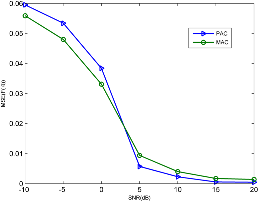
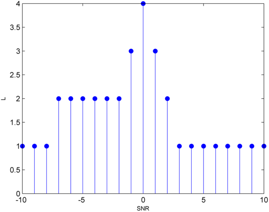
Subsequently, we evaluate the performance of the MAC scheme and compare it with that of the PAC scheme. Figure 9 shows the estimation performance in terms of MSE as a function of the number of groups. Specifically, we set $\mathrm{SNR}=5\mathrm{dB}$ and L = 5. As shown in Figure 9, the performance of the EMML estimator is always better than that of the MME, and it can achieve the CRLB with a large number of groups. Figure 10 compares the performance of the MAC scheme with that of the PAC scheme over different SNRs, where $F(\theta )=0.3$ , N = 500, and L = 5. Expectedly, a larger SNR leads to a better performance in both schemes. We also observe that the MAC scheme outperforms the PAC scheme when SNR is low and exhibits a degraded performance when SNR is high. This can be explained easily. As stated in section “Problem formulation,” the MAC scheme, wherein multiple sensors share a common channel, can effectively suppress the channel noise and hence reduce its uncertainty. Therefore, when the power of the channel noise is large, the MAC scheme can achieve a better performance than the PAC scheme. As the power of the channel noise decreases, the impact of channel noise on the estimation performance is also reduced. In this case, the superposition of impaired signals over fading channels may have a significant impact on the performance of the MAC scheme and subsequently lead to inferior performance as compared to the PAC scheme. Figure 11 compares the performance of the PAC scheme with that of the MAC scheme with different L, where $F(\theta )=0.3$ and $\mathrm{SNR}=0\mathrm{dB}$ . Expectedly, a larger N leads to a better performance in both schemes. We also observe that the MAC scheme with a larger group size exhibits a better performance. Figure 12 gives the optimal setting of L for different channel SNRs when the number of sensors is fixed at N = 300. As shown, when SNR is about zero, a higher L is needed to offer the minimum achievable MSE.

Figure 9.

MSE of $F(\theta )$ as a function of the number of groups.

Figure 10.

Comparison between the two schemes for various SNRs ( $F(\theta )=0.3$ , $N=500$ , and L = 5).

Figure 11.

MSE of $F(\theta )$ as a function of the number of sensors for both schemes ( $F(\theta )=0.3$ , $\mathrm{SNR}=0\mathrm{dB}$ ).

Figure 12.

Optimal setting of L for the MAC scheme (N = 300).

Table 1 shows the ratio of the EMML to the MME computation time for these two schemes. The MME is employed to solve linear moment equations and thus has lower complexity and takes less time. In contrast, the EMML estimator is generally complicated, since it requires a few iterations to alternate between the E step and M step. It is evident that the EM algorithm converges quickly in the PAC scheme and converges slowly in the MAC scheme. Moreover, in the MAC scheme, larger group size leads to slower convergence.

Table 1.

The ratio of the EMML to MME computation time $T_{\mathrm{EMML}}/T_{\mathrm{MME}}$ .

N	PAC	MAC
		L = 2	L = 4	L = 5
300	8.4	15.8	22.1	27.6
600	13.6	18.1	31.2	32.5

MME: method of moments estimator; PAC: parallel-access channel; MAC: multiple-access channel.

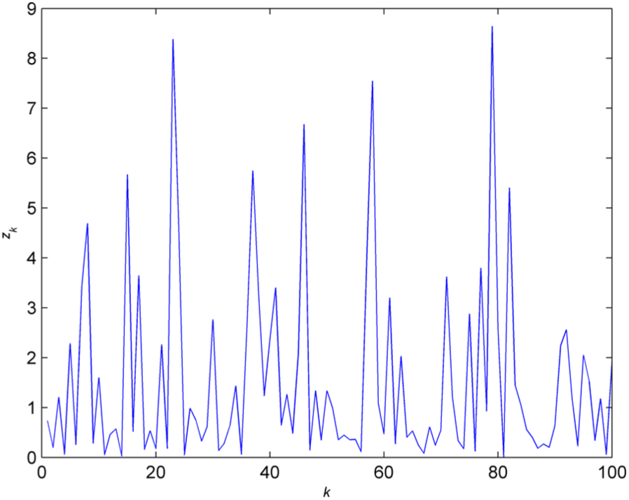
To better understand the convergence rate of the EM algorithm, we choose N = 300 and ${\sigma }_v=0.5$ and generate a realization of the received signals at the fusion center. Figures 13 and 14 give the received signal power at the fusion center for the PAC and MAC schemes, respectively. For the PAC scheme, the initial values of $\hat{F}(\theta )$ and ${\hat{\sigma }}_v$ are calculated by equations (38) and (39), and we have $\hat{F}(\theta {)}^0=0.2174$ and ${{\hat{\sigma }}^0}_v=0.5518$ . The EM algorithm converges to the values $\hat{F}(\theta )=0.3939$ and ${\hat{\sigma }}_v=0.4659$ . For the MAC scheme, the initial values of $\hat{F}(\theta )$ and ${\hat{\sigma }}_v$ are calculated by equations (55) and (56), and we have $\hat{F}(\theta {)}^0=0.2698$ and ${{\hat{\sigma }}^0}_v=0.6076$ . The EM algorithm converges to the values $\hat{F}(\theta )=0.3811$ and ${\hat{\sigma }}_v=0.4213$ . Figures 15 and 16 plot the values of $F(\theta )$ and ${\sigma }_v$ against the number of iterations for the PAC and MAC schemes, respectively. In order to compare the convergence rate of the EM algorithm with that of the traditional Newton–Raphson algorithm, the same initial values of $\hat{F}(\theta )$ and ${\hat{\sigma }}_v$ are adopted. For the PAC scheme, the EM algorithm requires 91 iterations, while the Newton–Raphson algorithm requires 13 iterations to converge to the same values. For the MAC scheme, the EM algorithm requires 129 iterations, while the Newton–Raphson algorithm requires 31 iterations to converge to the same values.

Figure 13.

The received signal power at the fusion center for the PAC scheme (N = 300).

Figure 14.

The received signal power at the fusion center for the MAC scheme (K = 100, L = 3).

Figure 15.

The values of $F(\theta )$ and ${\sigma }_v$ against the number of iterations for the PAC scheme (N = 300).

Figure 16.

The values of $F(\theta )$ and ${\sigma }_v$ against the number of iterations for the MAC scheme (K = 100, L = 3).

Apart from the number of iterations required for convergence, consistent convergence is also essential. The EM algorithm is guaranteed to converge to at least a local maximum. Unlike the EM algorithm, the Newton–Raphson algorithm is very sensitive to the initial value and sometimes fails to converge. When the initial value of $\hat{F}(\theta )$ is fixed, while ${{\hat{\sigma }}^0}_v\le 0.023$ for the PAC case and ${{\hat{\sigma }}^0}_v\le 0.051$ for the MAC case, the Newton–Raphson algorithm then fails to converge. However, the EM algorithm always converges to the ML estimates. In addition, to implement the Newton–Raphson algorithm, the second derivatives of the log-likelihood function are required in each iteration. In contrast, these are not required in the EM algorithm.

In these results, the local quantization threshold is prefixed arbitrarily for the sake of simplicity. In fact, the local threshold may have a direct impact on the estimation performance. Figure 17 shows the effect of the quantization threshold on the EMML estimator, where $\theta =1$ , ${\sigma }_n=1$ , N = 500, L = 2, and $\mathrm{SNR}=10\mathrm{dB}$ . For the PAC scheme, the minimum MSE is achieved when ${\tau }^{*}=1.3$ . For the MAC scheme, the minimum MSE is achieved when ${\tau }^{*}=1.8$ . As shown, the curve of MSE is very flat around ${\tau }^{*}$ . However, when the prefixed threshold is far away from ${\tau }^{*}$ , the estimation performance is very unsatisfactory. Figures 18 and 19 show the performance of the EMML estimator in terms of the worst-case MSE for the PAC and MAC schemes. We set $\Delta =1$ , ${\sigma }_n=1$ , and $\mathrm{SNR}=10\mathrm{dB}$ . The initial threshold is set to ${\tau }^0=3$ . Note that the smaller the worst-case MSE is, the better the performance is. The EMML estimator using the approximately optimal threshold ${\tau }_{\mathrm{app}}$ outperforms the one using the random threshold ${\tau }_{\mathrm{rand}}({\tau }_{\mathrm{rand}}~U(0,\Delta ))$ substantially. When the number of local sensors is large, the worst-case MSE of the EMML estimator using ${\tau }_{\mathrm{app}}$ is close to that using the optimal threshold ${\tau }_{\mathrm{opt}}$ . It implies that the threshold design based on the minmax CRLB criterion is feasible if the number of sensors is large.

Figure 17.

MSE of $\theta$ as a function of the threshold $\tau$ ( $\theta =1$ , ${\sigma }_n=1$ , SNR = 10 dB, N = 500, and L = 2).

Figure 18.

The worst-case MSE of $\theta$ as a function of the number of sensors for the PAC scheme ( $\Delta =1$ , ${\sigma }_n=1$ , SNR = 10 dB).

Figure 19.

The worst-case MSE of $\theta$ as a function of the number of sensors for the MAC scheme ( $\Delta =1$ , ${\sigma }_n=1$ , SNR = 10 dB, and L = 2).

Conclusion

In this work, we studied the problem of distributed parameter estimation in the PAC and MAC schemes. Considering one-bit quantization at local sensors and fading channels with unknown noise variance, we derived a ML estimator analytically based on the EM algorithm. Simulation results show that this estimator exhibits superior performance compared to the MME in both schemes. It is asymptotically unbiased and can attain the CRLB with a large number of sensors. In addition, we determined that when the noise power at the fusion center is large, the MAC scheme outperforms the PAC scheme but leads to slower convergence. Finally, to ensure accurate estimation over the entire parameter range, we adopted the minmax CRLB criterion to design the quantization threshold. Simulation results demonstrated the effectiveness of the approximately optimal threshold in terms of worst-case MSE.