Sage Journals: Discover world-class research

Abstract

In recent years, the foreign fibers in cotton lint significantly affect the quality of the final cotton textile products. It remains a challenging task to accurately distinguish foreign fibers from cotton. This article proposes an embedded system based on field programmable gate array (FPGA) + digital signal processor (DSP) to recognize and remove foreign fibers mixed in cotton. With substantial tests of this system, we collect massive samples of foreign fibers and fake foreign fibers. Based on these samples, a convolution neural network mode is developed to validate the classification of the suspected targets from the detection subsystem, to improve the detection reliability. After training several model architectures, we find a model with the best balance between performance and computation. The high success rate (up to 96% in the validation set) demonstrates the effectiveness of the model. Moreover, the computation time (5 ms on a single image based on an eight-core DSP) indicates the efficiency of the detection, which ensures the real-time application of the system.

Keywords

Deep learning foreign fiber embedded system TMS320C6678

Introduction

The foreign fibers include hair, ropes, plastic film, polypropylene twines, and so on which can seriously affect the quality of the final cotton textile products. How to accurately identify and eliminate the foreign fibers mixed in raw cotton is one of the most concerned focuses in the textile industry. In recent years, a variety of principles and various types of cotton fiber cleaning machine have come out. The main detecting principles can be categorized into three types: photoelectric detection, ultrasonic detection, and optical recognition. Based on the optical detection principle, computer vision techniques have the advantages of low cost, fine consistency, superior speed, good objectiveness, and high accuracy.^1,2 The working environment of the foreign fiber machine is usually high temperature, high humidity, and high dust, which means that very rigorous industrial standards are required for the foreign fiber machine, such as low power consumption and high reliability. In addition, the detection of different fibers requires real-time and stable work, so the calculation time of each processing step should be accurate enough and adjustable, to remove the fibers accurately. Therefore, a good system to remove cotton fiber should be suitable for low-cost, miniaturization and high-reliability design of cotton sorting equipment in cotton mills.³

A large number of algorithms have been proposed for foreign fiber in cotton extraction and classification,^{4

–15} which have been used in various applications. However, all these algorithms require manual participation to extract features and to design feature models. Besides the classic machine-learning technology, a new technology called deep learning (DL) has been more and more widely used recently.¹⁶ An obvious advantage of DL is feature learning, that is, the automatic feature extraction from the raw data, with the features from higher levels of the hierarchy being formed by the composition of lower level features.¹⁷

In this article, we proposed a real-time detection algorithm based on the classical machine learning and its implementation on an embedded system using DSP + FPGA. The system has a large number of cotton mills.¹⁸ The cotton flow speed in these mills ranges from 4 m/s to 15 m/s. These cotton mills are commonly used all over the world. We collect a large number of samples from different machines and different production lines and then label the samples in typical fiber classes, such as polypropylene, fluorescent fiber, and plastic sheeting. According to the characteristics of deep neural network and the requirement of real-time processing, we propose a model with the best balance between performance and computation. In addition, under the requirement of low cost and the stability of industrial scenarios, we propose a hybrid multicore scheduling algorithm for an eight-core DSP to improve the real-time performance of the CNN model in practical applications.

Materials and methods

Hardware

The system consists of a cotton pipeline, camera, light source, high-pressure spray valve, processing subsystem, industrial control computer, and removal subsystem, as shown in Figure 1

Figure 1.

System principle diagram.

The processing subsystem uses DSP + FPGA, which reduces the cost compared with the same level of graphics processing unit (GPU) architecture.¹⁹ This also improves the processing efficiency and enhances the adaptability of the system industrial scene. The imaging unit monitors the cotton flow passing through the channel. After finding the suspected fiber, the detection subsystem sends the target area to the confirmation subsystem based on the DL neural network. The confirmation subsystem sends the corresponding elimination instruction to the removal subsystem through the removal algorithm. The structure diagram of a foreign fiber cleaning machine is shown in Figure 2.

Figure 2.

Structure diagram of foreign fiber cleaning machine. (1) Flow direction, (2) cotton pipe, (3) cotton, (4) background board, (5) the imaging unit, (6) tube, (7) foreign fiber, (8) removal fan, (9) processing subsystem, (10) classification subsystem, (11) industry personal computer, (12) Internet, and (13) cloud server.

Detection subsystem

To extract targets quickly and accurately, detection algorithms usually adopt a strategy from simple to complex. In this article, target detection algorithms are summarized as shown in Figure 3.

Figure 3.

Flow chart of the target detection algorithm.

The first two steps are used to extract candidate regions from the whole image quickly and confirm them preliminarily, such as edge information. In the second step, the suspected targets in the first two steps are further confirmed using the fine features of foreign fibers, such as size, texture, area, and invariant moments. After acquiring the detection target area, the final foreign fiber detection result is obtained using the classifier based on a neural network to classify and recognize the target.

Considering the universality of the system, we also use the traditional statistical learning machine algorithm. According to the operation characteristics of the camera in the actual equipment and considering the influence of the environment on the optical path, we use the following image features for statistical learning:

In white light, ultraviolet light, and polarization, there are the color difference or edge gradient difference between foreign fibers and cotton.

The number of foreign fibers is smaller than cotton, so cotton and background account for the main part of data statistics.

When cotton changes, the cotton part of the image will change, but the proportion of foreign fibers in the total is still small.

According to the different materials of foreign fibers, as well as the transverse wind speed of the whole cotton flow pipeline and the size of cotton, there are differences in the actual foreign fibers speed.

Based on the above image features, we design the detection algorithm flow as shown in Figure 4. The algorithm has good performance in the field environment of the complex cotton flow channel and also has strong adaptability to multi-light path and anti-interference ability.

Figure 4.

Flow chart of fiber detection algorithms.

The camera sends RGB raw data to the FPGA by Camera Link. The FPGA converts the RGB raw data into three channels: (1) RGB raw data. (2) In cotton flow, the direction of foreign fibers is random, so we use the Laplace operator to calculate gradient information in our system design. The operator is a simple implementation and rotation invariance. The standard Laplace transform of a two-dimensional (2-D) image function is the second derivative of isotropy. The discrete form as formula (1)

\nabla^{2} f (x, y) = f (x + 1, y) + f (x - 1, y) + f (x, y + 1) + f (x, y - 1) - 4 f (x, y)

The operator always represented as a matrix $[\begin{matrix} 0 & 1 & 0 \\ 1 & - 4 & 1 \\ 0 & 1 & 0 \end{matrix}]$ . The standard Laplace operator deals with images, which is the same horizontal and vertical resolution. But in our system, horizontal resolution is greater than the vertical, so we appropriately increase the number of transverse processing points and improve the Laplace operator as a matrix $[\begin{matrix} 0 & 2 & 3 \\ 1 & - 4 & - 6 \\ 0 & 2 & 3 \end{matrix} \begin{matrix} 5 \\ - 12 \\ 5 \end{matrix} \begin{matrix} 3 & 2 & 0 \\ - 6 & - 4 & 1 \\ 3 & 2 & 0 \end{matrix}]$ . 3. Using the difference between foreign fibers and cotton in color space. In color difference detection, the image of original RGB data is transformed into Lab space that has well correlations with the human visual experience. Formulas (2) to (6) indicate how RGB is transmitted to Lab space. Based on the definition of Lab uniform color space by the International Institute of Illumination (Commission Internationale de L’Eclairage [in French]), the color difference between two points can be expressed as formula (7)

[\begin{matrix} X \\ Y \\ Z \end{matrix}] = [\begin{matrix} 0.412453 & 0.357580 & 0.180423 \\ 0.212671 & 0.715160 & 0.072169 \\ 0.019334 & 0.119193 & 0.950227 \end{matrix}] [\begin{matrix} R \\ G \\ B \end{matrix}]

L = 116 f (\frac{Y}{Y_{n}}) - 16

a = 500 [f (\frac{X}{X_{n}}) - f (\frac{Y}{Y_{n}})]

b = 200 [f (\frac{Y}{Y_{n}}) - f (\frac{Z}{Z_{n}})]

f (t) = {\begin{matrix} t^{\frac{1}{3}}, & if t > {(\frac{6}{29})}^{3} \\ \frac{1}{3} {(\frac{6}{29})}^{2} t + \frac{4}{29} & otherwise \end{matrix}

In formulas (3) to (5), the default value of $X_{n}, Y_{n}, and Z_{n}$ is 95.047, 100.0, and 108.883, respectively.

E_{a b} = \sqrt{{(Δ L)}^{2} + {(Δ a)}^{2} + {(Δ b)}^{2}}

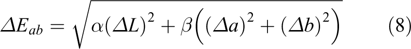
In formula (7), ▵L represents the L difference between two points, ▵a represents the a difference between two points, and ▵b represents the b difference between two points. Considering the working condition of foreign fiber machine, we introduce the weight of channel differences: $α, β$ for different illumination, modify formula (7) to

Δ E_{a b} = \sqrt{α {(Δ L)}^{2} + β ({(Δ a)}^{2} + {(Δ b)}^{2})} ​

while $α + β = 1, 0 < α < 1, 0 < β < 1.$

After the above three kinds of data are transferred from FPGA to DSP, the system starts the target detection algorithm. It is always difficult to select the reasonable threshold of binary segmentation in target detection. Maximum class square error method designed by Nobuyuki Otsu (OTSU) is a common threshold selection method, but it is very sensitive to noise and target size and only effective for images with a single peak of between-class variance. In the foreign fiber machine system, cotton flow and background are the main parts of the image, with foreign fibers only a few. Threshold extracted by OTSU method cannot effectively segment foreign fibers and cotton. If we use more complex threshold selection method, the computation will be greatly increased, which is not conducive to the real-time implementation of the system. Consider the above problems, we use simple statistical learning to extract the threshold. In the cotton flow, we believe that the probability of foreign fibers should be less than 0.5%–1% of cotton, so we expose the probability parameter ε to the users. The system calculates the statistics of the gradient and color histogram in the idle state (formulas (9) and (10)) and calculates the summation threshold according to the probability parameter ε (formulas (11) and (12)), then we count the color difference and gradient data inversely from the maximum value (255), and the actual segmentation threshold of the color difference and gradient data can be obtained when the closest summation threshold is reached, as shown in Figure 5. After obtaining the threshold, we use it to binarize the gradient and color difference data and combine these result for detection, as shown in Figure 6

{Sum}_{G} = \sum_{h = 0}^{H - 1} \sum_{w = 0}^{W - 1} \nabla^{2} f (h, w)

{Sum}_{c} = \sum_{h = 0}^{H - 1} \sum_{w = 0}^{W - 1} Δ E_{a b} (h, w)

{Sum}_{{thrd}_{G}} = {Sum}_{G} * ε

{Sum}_{{thrd}_{c}} = {Sum}_{c} * ε

Figure 5.

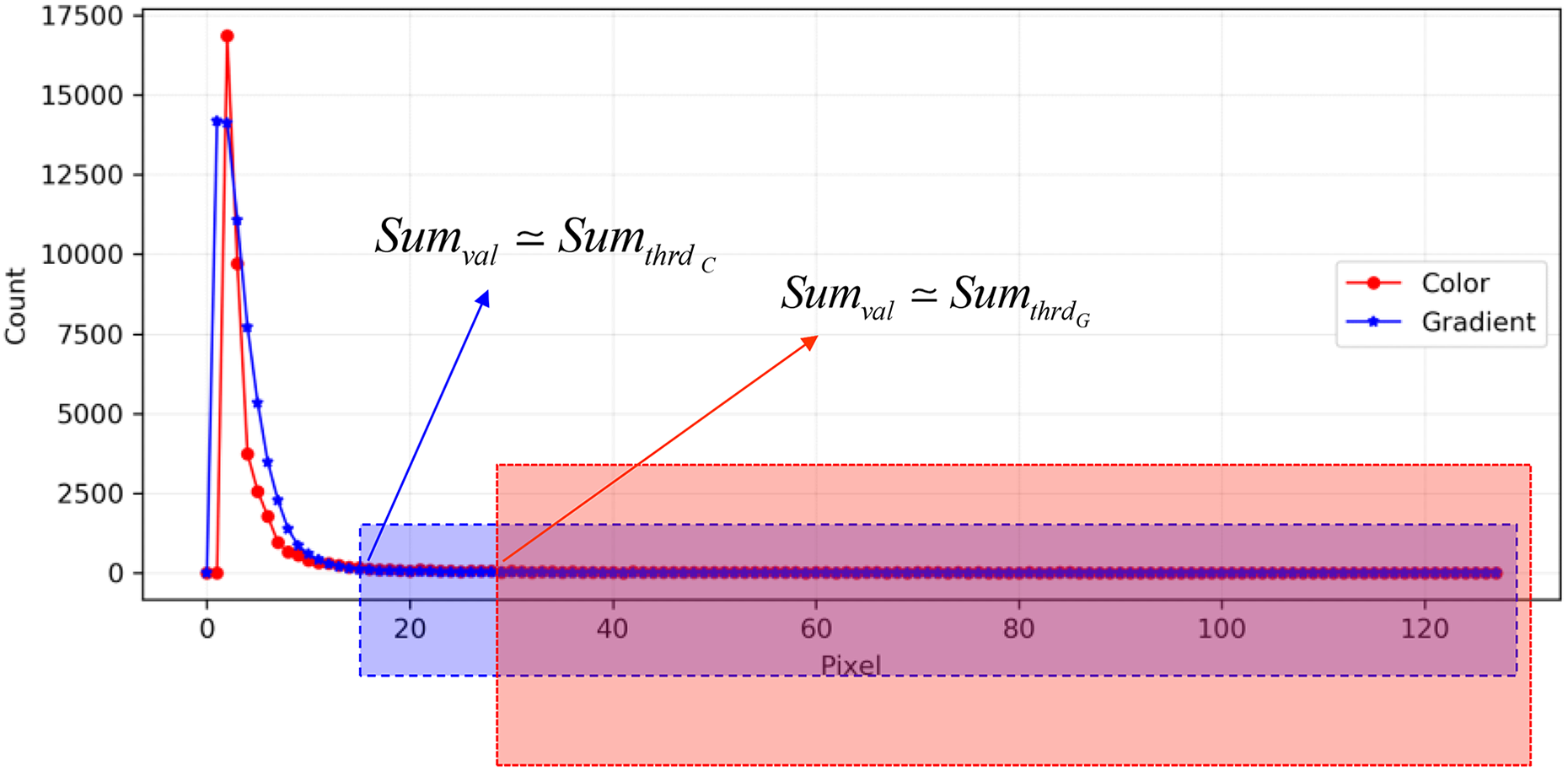
The process of threshold extraction.

Figure 6.

(a) Example with target and (b) example with no target.

Image classification

In the classification and recognition algorithm of foreign fibers, we use the idea based on DL. The basic DL tool used in this work is the convolution neural networks (CNNs).²⁰ The current strategy commonly used for extracting the CNN features is to use the existing large CNN-based training data sets, such as IMAGENET,²¹ to extract the feature as described in previous studies.^22
–24 This is actually a typical transfer learning strategy, which can work well when the tested images are similar to the original data sets for the CNN training. However, this transfer learning strategy could not work efficiently in our study since the IMAGENET data sets are not similar to the data sets we use currently. Therefore, we have to train a new CNN model using our fiber sample data sets. For this sake, we need a good CNN architecture. Unfortunately, the commonly used CNN architecture is not suitable for our case due to two aspects. First, the commonly used CNN architecture usually has a very deep structure, which will cause over-fitting problems due to our limited fiber data sets. Second, it is time-consuming when using this deep structure for the feature extraction, which makes it not suitable for real-time applications in the practical industrial field. Thus, we design a new CNN architecture as shown in Figure 7.

Figure 7.

CNN architecture for our system. CNN: convolution neural network.

As shown in Figure 7 and Table 1, our CNN structure consists of seven convolution layers, one global avgpool layer, one Softmax layer, and does not have a fully connect layer. Two Maxpool layers are added into Conv1 and Conv3 to downsample for not only reducing the parameters but also retaining the most useful sampled features, and a rectified linear unit (ReLU) is also adopted at all the convolution layers. Next, a global avgpool layer combined with a Softmax classifier is implanted to output the classification result for the specific input image. The designed CNN structure can not only improve computational performance but also lead to good segment effects on the background and cotton.

Table 1.

General outline of our CNN architecture.

Label	Type	Filters	Size/stride/pad	Output
—	Input	—	—	128 × 128 × 3
Conv1	Convolutional	32	3 × 3/1/1	128 × 128 × 32
Conv1	Maxpool	—	2 × 2/2/0	64 × 64 × 32
Conv2	Convolutional	16	1 × 1/1/0	64 × 64 × 16
Conv3	Convolutional	64	3 × 3/1/1	64 × 4 × 64
Conv3	Maxpool	—	2 × 2/2/0	32 × 32 × 64
Conv4	Convolutional	32	1 × 1/1/0	32 × 32 × 32
Conv5	Convolutional	128	3 × 3/1/1	32 × 32 × 128
Conv6	Convolutional	64	1 × 1/1/0	32 × 32 × 64
Conv7	Convolutional	10	1 × 1/1/0	32 × 32 × 10
GlobalAvgpool	Avgpool	—	—	10
Softmax	Softmax	—	—	10

CNN: convolution neural network.

Convolution layer is the basic component of CNN. The parameters of the convolution layer are composed of a set of learnable kernels. For example, if we use a 2-D image I as our input, we probably also want to use a 2-D kernel K

S (i, j) = (I \times K) (i, j) = \sum_{m} \sum_{n} I (m, n) K (i - m, j - n)

Formula (13) can also be written as formula (14)

S (i, j) = (I \times K) (i, j) = \sum_{m} \sum_{n} I (i - m, j - n) K (m, n)

Similarly, in the case of 3-D convolution layer l, assume the input data are $I^{l} \in ℝ^{H^{l} \times W^{l} \times D^{l}}$ , the learnable kernel of this layer is $K^{l} \in ℝ^{H \times W \times D^{l}}$ , convolution operation in 3-D only extends 2-D convolution to all corresponding channels. Finally, the sum of $H \times W \times D^{l}$ elements in the convolution process is taken as the result, as shown in formula (15)

y_{i^{l + 1}, j^{l + 1}, d} = \sum_{i = 0}^{H} \sum_{j = 0}^{W} \sum_{d^{l} = 0}^{D^{l}} K_{i, j, d^{l}, d} \times I_{i^{l + 1} + i, j^{l + 1} + j, d^{l}}^{l}

While $(i^{l + 1}, j^{l + 1})$ is the position coordinate of the convolution result, satisfying the following formulas (16) and (17)

0 \leq i^{l + 1} < H^{l} - H + 1 = H^{l + 1}

0 \leq j^{l + 1} < W^{l} - W + 1 = W^{l + 1}

The hyperparameters of the convolution layer mainly include the size of the convolution kernel, the stride of convolution operation, and the number of convolution kernels. The convolution kernel size usually is small, such as $3 \times 3$ or $1 \times 1$ . Compared with large size, the small one enhances the capacity of the CNN and the complexity of the model. More important, it can effectively reduce the number of parameters and the amount of computation. So our system mainly uses $3 \times 3$ and $1 \times 1$ convolution, the stride of the convolution operation usually set as 1, as shown in Figure 7. In addition, padding operation can be used before convolution operation, which is mainly used to process the edge information of input data and keep the size of input and output.

ReLUs are used as a substitute for saturating nonlinearities. This activation function adaptively learns the parameters of rectifiers and improves accuracy at a negligible extra computational cost. It is defined as formula (18)

f (y_{l}) = {\begin{matrix} 0, y_{l} < 0 \\ y_{l}, y_{l} \geq 0 \end{matrix}

where y_l represents the input of the nonlinear activation function f on the l-th channel.

The most common classification objective function in CNN is Softmax, also called cross-entropy loss function, as shown in formula (19). It is mainly used to characterize the probability of output results in different classes

L_{cross-entropy} = L_{softmax} = - \frac{1}{N} \sum_{i = 1}^{N} log (\frac{e^{h_{y_{i}}}}{\sum_{j = 1}^{C} e^{h_{j}}})

N represents the total number of samples per training, y_i is the real class label of sample i, h refers to the final output of the network or the predicted result of sample i by the designed network, and C represents the number of classes, which is 10 in our system.

Training and testing data sets

The training set pictures of different fibers have their own particularities. For example, most of the fibers are concentrated in the center of the samples. The distribution patterns of the cotton and background are unified to a certain extent, where several kinds of different fibers locate. The database used here includes 10 different classes, and each class has 76,421 training samples and 19,106 valid samples, as shown in Table 2 and Figure 8.

Table 2.

Descriptions and quantitative data of the database images.

Harmness	Class	Common name	Images (count)	10–12 m/sConditions (%)	5–7 m/sConditions (%)
Real	cf_0	polypropylene	19450	46	54
	cf_1	mulch film	6140	30	70
	cf_2	Paper	6134	56	44
	cf_3	feather	7140	48	52
	cf_4	cloth	6200	56	44
	cf_5	fluorescence	8941	44	56
	cf_6	transparency film	7994	25	75
Pseudo	cnf_7	cottonseed	12663	51	49
	cnf_8	cotton stalk	11041	44	56
	cnf_9	yellow cotton	9824	54	46

Figure 8.

Samples of images in different classes. cf_0: polypropylene, cf_1: mulch film, cf_2: paper, cf_3: feather, cf_4: cloth, cf_5: fluorescence, cf_6: transparency film, cnf_7: cottonseed, cnf_8: cotton stalk, cnf_9: yellow cotton, cf_0–cf_6: real fiber, cnf_8–cnf_9: fake foreign fiber.

The entire database is initially divided into two data sets, that is, the training set and the testing set, which is carried out by randomly splitting the 95,527 images so that 80% of them form the training set, and the rest 20% form the testing set. The 80/20 splitting ratio of the training/testing data sets is the most commonly used one in current neural network applications. Note that other similar splitting ratios (e.g. 75/25 or 70/30) would not lead to significant discrepancies on the performance of the developed models.²⁵

We use the standard stochastic gradient descent algorithm²⁶ to learn the parameter determination of the proposed CNN, which includes a feed-forward pass stage and a back propagation pass stage. The learning algorithm of CNN is shown in Algorithm 1.

Algorithm 1.

Learning process of the fiber classification CNN $h_{θ} (x)$ .

Augmentation process

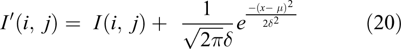
The main purpose of applying augmentation is to increase the data sets and introduce slight distortion into the images, which helps reduce over-fitting during the training stage. In machine learning, over-fitting appears when a statistical model describes random noise or error rather than the underlying relationship.²⁷ In our foreign fiber data sets, considering that the position of the camera in practical application is fixed, we only use 90°, 180°, 270° among the random flip. Then, we add random white noise and randomly change the ambiguity of the image to expand the data set, as shown in Figure 9. Figure 9(a) represents the resulting images obtained by applying random noise transformation on the train image. Figure 9(b) visualizes the simple rotation of the input image. Figure 9(c) represents the input image blurred by random Gauss filter with different parameters. Figure 9(d) represents the resulting images obtained by applying random brightness of the input image. The last row represents the random augmentation process during the training stage.

Figure 9.

An example of data augmentation process: (a) random noise addition, (b) random rotation, (c) random blur, (d) random change brightness, and (e) image augmentation with process (a)–(d).

The formula of noise operation is as follows

I^{'} (i, j) = I (i, j) + \frac{1}{\sqrt{2 π} δ} e^{\frac{- {(x - μ)}^{2}}{2 δ^{2}}}

$I (i, j)$ represents the input image pixel at position $(i, j)$ , μ and δ refer to mean value and variance of the Gaussian distribution, respectively, and x is the random value between 0 and 1.

The rotation operation is shown in formula (21)

I^{'} (i, j) = I (i, j) \times [\begin{matrix} cos θ & sin θ & 0 \\ - sin θ & cos θ & 0 \\ 0 & 0 & 1 \end{matrix}]

In formula (21), θ is the rotation angle, $0 \leq θ \leq 360^{\circ}$ . In our system, we choose the rotation angle as 0°, 90°, 180°, and 270°.

Blur operation means that we use the Gaussian kernel with radius R to calculate an inner product with the original image to get the blurred image, as shown in formula (22); in our system, we choose randomly in radius 3, 5, 7, and 9.

g (x, y, σ) = \frac{1}{2 π σ^{2}} e^{- \frac{(x^{2} + y^{2})}{2 σ^{2}}}

0 \leq x \leq R

0 \leq y \leq R

I^{'} (i, j) = I (i, j) \otimes g (x, y, σ)

Results

The training set and the testing set are sampled during different time spans and different factories to increase diversity. The time interval is more than 1 year, and the factory location covers most of the provinces in mainland China. To train the model, we manually annotate 95,527 samples as shown in Figure 8. The learning rate follows a specific annealing schedule, which starts from 0.1 and descends following the equation

{learning}_{rate} = {learning}_{rate} \times {(1 - (Batch_num) / Batch_max)}^{power}

In formula (26), $Batch_num$ represents the current batch number, $Batch_max$ denotes the maximum batch size, and $power$ is the hyperparameter. In this article, we use a value of 4 for the hyperparameter.

The CNN model is trained using the training hyperparameters as presented in Table 3. A single PC was used for the entire process of training and testing the foreign fiber classification model described in this article. Training of the CNN has performed in the GPU mode. Every training iteration took approximately 12 h on this specified machine whose basic characteristics are presented in Table 4.

Table 3.

Training hyperparameters.

Hyperparameter	Value
Max batches	238,815
Batch size	128
Start learning rate	0.1
Power	4

Table 4.

Basic machine characteristics.

Hardware and software	Characteristics
Memory	16 GB
Processor	Intel(R) Xeon(R) E5-2620 v4 at 2.10 GHz
Graphics	NVIDIA GeForce GTX 1080 Ti
Operating system	Linux Ubuntu 16.04 64 bits
Language and components	C + NVIDIA cuDNN + NVIDIA CUDA

Figure 10 shows the average loss and valid accuracy in top1 and top2 on the training during each epoch after 300 epochs trained, the average loss declined not obvious. Besides, the classification accuracy of top1 and top2 in the validation data sets reached more than 94%, so we considered that the trained model was able to use in our system. Figure 11 shows classification cases of the randomly selected images throughout the validation data sets. Figure 11(a) shows samples of correct classification and Figure 11(b) shows samples of some errors in the classification of our model. From the error classification result of the images, it is more in line with our classification expectations. In the practical application of our system, we can judge them to be or not to be true foreign fibers under the top2 situation and classic detection algorithms.

Figure 10.

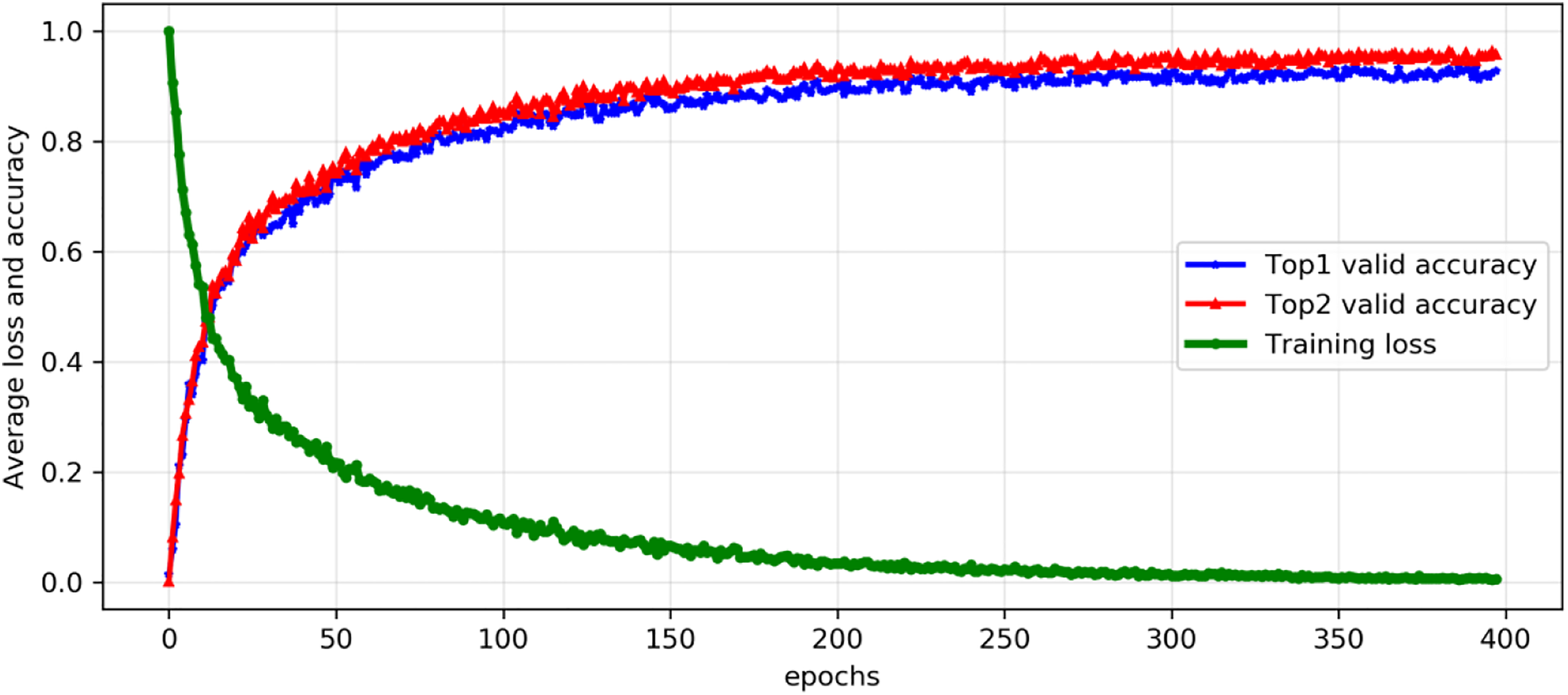
Average loss and valid accuracy during each epoch.

Figure 11.

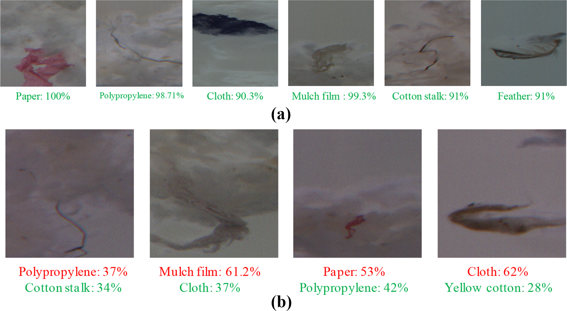
Examples of the classification result of various images throughout the validation datasets: (a) samples of correct classification and (b) samples of some errors in classification. The red label is an error, and the green one is correct.

Design and implementation

In the industrial application of machine vision, the common hardware options are central processing unit (CPU), advanced RISC machine (ARM), graphics processing unit (GPU), FPGA, DSP, and so on. The applications and comparisons among them are summarized below:

Compared with CPU and ARM, DSP, the FPGA and GPU have great advantages in large-scale mathematical operations.^28

–34 However, GPU is mainly manufactured by NVIDIA (Santa Clara, California) manufacturers, which does not provide driver source code and needs to bind with ARM or CPU. In addition, the operating system has to be Windows or Linux, which are not real time.

In power consumption, FPGA and DSP also have advantages against GPU in high-performance computation.

Compared with FPGA, DSP has advantages in software upgrade, development, and maintenance.

Considering the power consumption, the real-time requirement of the system, as well as the difficulty of software development and maintenance, we choose the embedded processing system based on FPGA + DSP for the design in this study.

The DL algorithm is generally implemented on PC by MATLAB or Python, which costs a lot of time since the convolution layer is time-consuming. GPU can significantly improve computation efficiency but does not fix the industrial environment as discussed above. Based on the architecture of DSP + FPGA, we optimize the program and obtain better performance.

In this article, we implement the algorithm on the TMS320C6678 multicore platform.³⁵ We combine the C language with linear assembly language to implement the forward algorithm in DL. Moreover, we use a multicore system based on DSP to achieve the best performance.

Multicore scheduling algorithm

According to the characteristics of DSP, we design a multicore scheduler algorithm based on TMS320C6678. Based on the multicore DSP applications, static scheduling is usually used, which is called as “the specified core does the specified things.”³⁶ Sometimes the tasks are statically assigned to processors, and the tasks within each processor are scheduled by a local scheduler, which makes the application development simple and more convenient for debugging. However, static scheduling is against load balancing. Therefore, if one wants to take full advantage of the inter-core parallelism, he needs to split the specified application into roughly equal parts. But for some specific applications, such as the CNN classification algorithm, the data between layers are strictly dependent, thus it often comes out that some cores are very busy, while the others are in idle waiting. Unlike static scheduling, dynamic scheduling is applied to many multicore systems, such as the load balancing algorithms in the Linux systems.³⁷ This scheduling method is beneficial to load balance because it can be simply summarized as doing uncertain things for uncertain cores. Dynamic scheduling can automatically adjust the capacity of each core to achieve balance. However, there are uncertainties in dynamic scheduling, which makes it difficult to debug or develop. Moreover, the cache resources are not fully utilized, and the work performed by each core often varies greatly, which makes the program and the data in cache stay constantly refreshed, and thus reduces the efficiency. Taking into account the advantages of the DSP, we design a hybrid scheduling algorithm to make full use of the cache mechanism.

Embedded systems usually adopt the concept of the task to form a multitask system. In this case, each task has its own context space, so it runs safely. However, the efficiency of context switching among the multitasks is low, which is not conducive to the real-time performance of the system. Therefore, in the design of the DSP scheduling algorithm, we adopt the software interrupt (SWI) mode that is similar to hardware interrupt. All SWI modes have a unified context space with high context switching efficiency. The more parallel the tasks are, the more obvious the efficiency advantage is.

The inter-core message is used interactively among multicore subsystems. Combining inter-core message with hardware navigation queue peculiar to TMS320C6678, we design a hardware-managed inter-core message queue. Each inter-core message can send a 32-bit message, which only bears an address of the shared memory so that the multicore subsystem does not have any barrier access.

For multicore software systems, the computation applications are divided into parallel parts so that they can be executed to make full use of multicore parallel processing capabilities. However, in multicore systems, an application is not the only serial in time, but also dependent on running space. In this article, we define the application parts that can be decomposed independently by the application layer tasks as a “job.” The execution of a job is not disorderly. There are strict constraints among them, which are called as a dependency. Dependency describes the order of execution among jobs, which mainly include the constrained entities of the previous job, that is, the jobs that are executed before the execution of the current job. Dependency dynamically allocates the sub-core resources according to the actual algorithm and splits the job statically, which maximizes the efficiency of the cache resources and the shared memory access.

Software design

TMS320C6678 consists of eight sub-C66 cores with a maximum dominant frequency of 1.4 GHz. Each core contains 32 KL1P, 32 KL1D, 512 KL2, and 4 MB of shared memory.³⁵ We named eight sub-cores numbered as 0–7, and the core 0 is responsible for scheduling and interfaces, such as network access, data access, which is called as “master core,” while the cores 1–7 are responsible for job execution as “slave core,” as shown in Figure 12.

Figure 12.

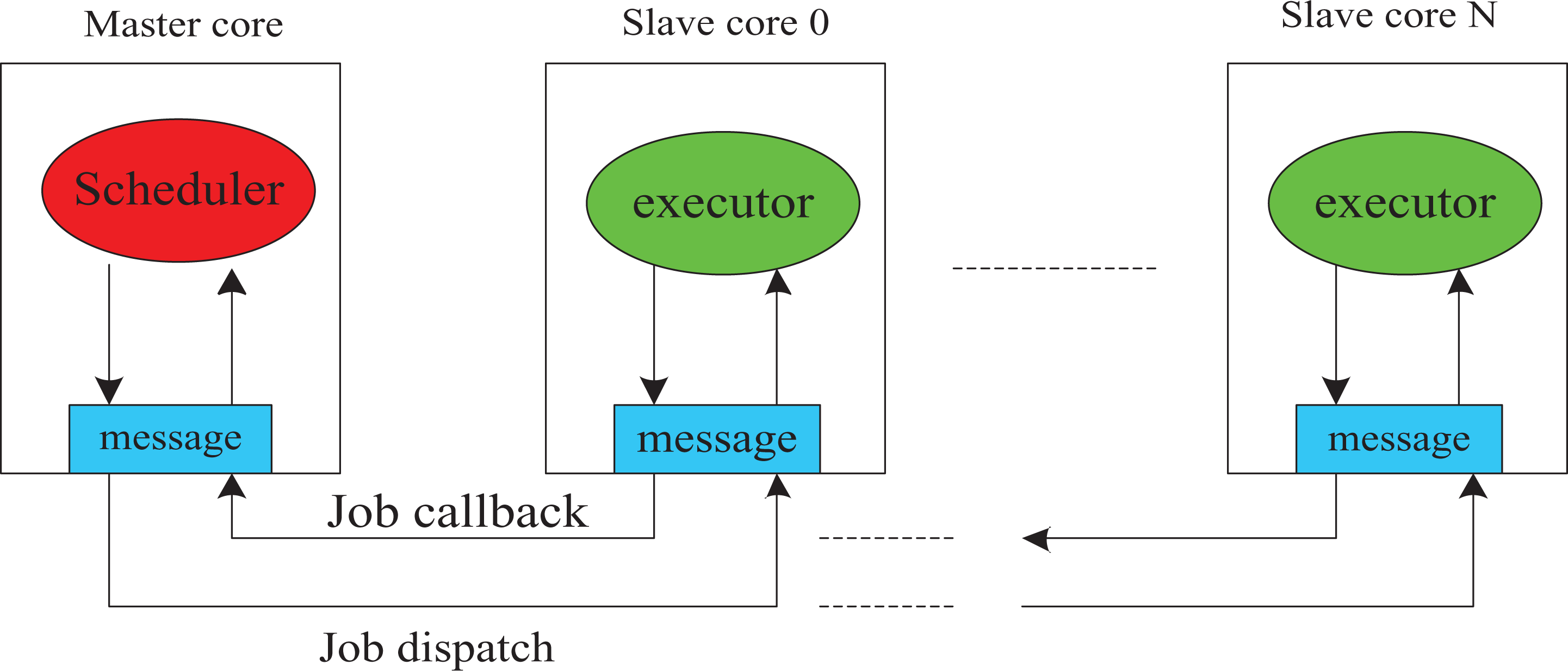
Scheduler and executor.

The soft hybrid scheduler is composed of function, interrupt handler, hardware queue, configuration program, and scheduling algorithm. As shown in Figure 13, the job usually has five states, which are Waiting, Ready, Execution, End, and Null.

Figure 13.

Soft hybrid scheduler.

The Waiting state means the job has just been generated and stored in the job list. The job needs to wait for the execution of all the other higher level jobs in the stored job list. When the higher level job is finished or there is no higher level of job independence, the scheduler will execute the dispatch algorithm. If there is an idle slave core, the job will be arranged to the target slave core execute, otherwise, it will enter into the ready state.

The Ready state denotes that job has entered into the job’s dispatch queue, and the dependency has been lifted, but at present, all slave cores are in busy. The job is waiting for the slave core resources in the dispatch queue. When the slave core resources are available, the job enters into the execution state.

The Execution state means that the job has been mapped into the running map, that is, a slave core is executing the job. After the slave core’s execution is done, the scheduler executes the callback operation. Once the job’s execution is finished, it enters into the end state.

The End state means the job is stored in the callback list and the corresponding execution is done, but some follow-up work is needed, for example, updating the dependency of the next job.

In the Null state, the job releases resources.

According to the above descriptions, the key factors of the scheduler’s efficiency depend on the job dispatch and execution request. In the computation process, each job expects to be executed as soon as possible. Therefore, if an idle slave core is available, the scheduler will dispatch work immediately to the slave core for the job execution. If no idle slave core is available, the job will enter into the corresponding dispatch queue and ready state. When the idle core appears, that is to say, the master core receives the slave core idle message for the first time, the master core will remove the high priority job from the job’s dispatch queue and send it to the slave core. In a word, under this mechanism, all the waiting jobs are always the earliest to be executed, and all the idle slave cores are always the earliest to get a job, which guarantees the efficiency of the scheduler.

Combining the CNN classification algorithm with the hybrid scheduler and the static scheduler, we design a typically hidden layer in the parallel job with our CNN architecture which is described in Table 1. The structures of the type 2 schedules are shown in Figure 14.

Figure 14.

The different scheduler and its utilization in eight cores of TMS320C6678: (a) static scheduler, (b) hybrid scheduler, and (c) hybrid scheduler and static scheduler of DSP utilization in eight cores.

As can be seen from Figure 14(a), the static scheduling algorithm divides the input image into eight parts (corresponding to eight cores), allocates the same resources to eight cores in system design, and divides the convolution operation into eight parts to carry out their respective CNN algorithms. In addition, considering the overlapping part of the convolution operation, we need to add several additional rows of overlapping data. Figure 14(b) shows the flow of the hybrid scheduling algorithm in the system. When the CNN algorithm operates at each layer, the computing units are dynamically allocated according to the given eight-core idle situation, so that the idle core can enter the bus state at any time, and the utilization of multicore can be fully improved. Figure 14(c) shows the eight-core utilization percentage of the two algorithms under a given 1000 pictures. In some cases, the utilization percentage of the static scheduling algorithm will be reduced to less than 70%. The main reason is that the static scheduling algorithm sets the specified core to do the specified things, other idle core resources cannot be fully utilized in these cases. However, in this case, the hybrid scheduling algorithm uses multicore resource management to avoid the long waiting of idle cores and divides the computing units according to the number of idle cores, thus fully improving the utilization of multicore.

To improve the ability of DSP, not only the efficient multicore scheduling mechanism but also the reasonable memory allocation is needed. In this system, we mainly use half of L2 for the L2 cache, which can greatly improve the cache capacity. The other half of the L2 is used for each slave core’s stack space as the temporary variable usage area in the job: 4 MB on-chip shared memory is accessible to all cores, so there will be bus conflicts when multicores access data at the same time. Nevertheless, the in-chip shared memory accessing speed is higher than DDR3. We can put the static tables used in the algorithm and the trained CNN weights into the shared memory in-chip.

Experiments

Hardware experiment and analysis

We use the same DL algorithm on the personal computer (PC) and DSP for the same images that need to be predicted, and the statistical calculation time is presented in Table 5. The PC is configured as i7 2600 at 3.4 GHz, 8 GB DDR3, and the DSP uses TI’s c6678 multicore platform with 1.25 GHz main frequency and 2 GB DDR3.

Table 5.

Performance between PC and DSP.

Type	Filters	Output	PC (ms)	DSP (ms)
Convolutional	32	128 × 128 × 32	7.075	0.573
Maxpool	—	64 × 64 × 32	3.303	0.675
Convolutional	16	64 × 64 × 16	1.162	0.235
Convolutional	64	64 × 64 × 64	11.581	0.586
Maxpool	—	32 × 32 × 64	1.373	0.379
Convolutional	32	32 × 32 × 32	0.809	0.201
Convolutional	128	32 × 32 × 128	10.506	0.420
Convolutional	64	32 × 32 × 64	2.557	0.564
Convolutional	10	32 × 232 × 10	0.457	0.063
Avgpool	—	10	0.034	0.02
Softmax	—	10	0.783	0.0006
Count	—	—	39.64	3.718

The actual velocity of the cotton flow is between 4 m/s and 14 m/s, and the distance between the valve and camera is 350 mm in our machine. The time of detection and classification ranges from 25 ms to 87 ms. Therefore, our design satisfies the real-time requirements.

Classification of foreign fibers

The equipment installed on the practical production line is shown in Figure 15. The tested production line is 350–500 kg/h, and the cotton speed ranges from 8 m/s to 14 m/s. The tested foreign fiber samples are shown in Figure 16. Corresponding results from the testing cases are shown in Table 6.

Figure 15.

Test production line. (a) 8–10 m/s and (b) 12–14 m/s.

Figure 16.

Typical foreign fibers: (a) polypropylene, (b) paper, (c) feather, (d) cotton stalk, (e) fluorescence, (f) mulch film, (g) transparency film, and (h) cloth.

Table 6.

Classification results of the system.

Foreign fiber class	Classification results/clean results										NO	ACC (%)
Foreign fiber class	cf_0	cf_1	cf_2	cf_3	cf_4	cf_5	cf_6	cnf_7	cnf_8	cnf_9	NO	ACC (%)
(cf_0) polypropylene	50										50	100
(cf_1)mulch film		50									50	100
(cf_2)paper		1	48	1							50	96
(cf_3)feather	1			49							50	98
(cf_4)cloth			4	1	45						50	90
(cf_5)fluorescence						50					50	100
(cf_6) transparency film							50				50	100
(cnf_7) cottonseed				1				49			50	98
(cnf_8)cotton stalk	2								48		50	96
(cnf_9)yellow cotton										50	50	100
Average												97.8

NO: total number of each class; ACC: lassify accuracy(in percentage) of each class.

The success rate reaches up to 97.8% for the model test. For the 500 testing samples, only nine samples’ classes were not correctly identified by the CNN model. Among the nine misclassified samples, several faulty ones contained similar artificial features. In these specific cases, the faulty images were registered in the class cnf_8 (cotton stalk, green one), but the network identified it as the cf_0 (polypropylene, red one), which are shown in the classification tables in Figure 17.

Figure 17.

The faulty classification results.

As shown in Figure 17, the cotton stalk is very similar to some polypropylene in human vision. However, the overall shape of the cotton stalk and the wrapping state in the cotton flow are different from the polypropylene. The model can easily extract features from most stalks, but the network itself is not sure about the misclassified stalks. In the practical operation process, we will further consider the case that treats the polypropylene as a real foreign fiber to be removed, to avoid missing real foreign fibers. In addition, paper and some cloth foreign fibers turn out easily misidentified, as shown in Figure 17. In general, the ultraviolet, transparent film, mulch film, feather, and colored polypropylene are also easy to classify because of their obvious characteristics.

Deployment

In our study, we deploy a system with classification subsystem and a system without classification subsystem in a factory in Yuncheng County, Heze City, Shandong Province, China, as shown in Figure 18. The main foreign fibers are gray polypropylene filament and transparent film. Without the classification subsystem, the number of hits per hour is about 2800 times, and among them, 80% are cotton stalks, which are very close to the polypropylene filament in the image, as shown in Figure 19(c). After appending the classification subsystem, the interference of cotton stalk and yellow cotton is effectively eliminated, and the number of strikes is reduced by around 85%. The real foreign fibers account for a large proportion, while the pseudo foreign fibers do not exist. The main reason is that when they pass through the classification subsystem, the subsystem cannot distinguish whether they belong to the pseudo foreign fibers or the real foreign fibers merely from the image.

Figure 18.

The deployment of the system in the production line: a machine (a) with and (b) without a classification subsystem.

Figure 19.

Actual strike count in the production line with classification subsystem or without it and the foreign fiber removal strategy. (a) Strike count with classification subsystem, 450 per hour. (b) Strike count without classification subsystem, 2800 per hour. (c) Image classification results rank second is polypropylene, and the classification score has reached 37.3%. In practice, we will consider that such results belong to real foreign fibers, which need to be removed.

Conclusions

In this article, we develop a foreign fiber sorting system based on DSP and FPGA. After collecting foreign fiber pictures in different environments, we create a sample library containing 95,527 typical foreign fibers. By considering the working environment of the foreign fiber cleaning machine, we design a CNN model that can best balance the performance and computation and deploy the model on multicore DSP. The high success rate up to 96% for the validation demonstrates the effectiveness of the model. In addition, we propose a hybrid scheduling algorithm based on the multicore DSP, which makes full use of cache resources, and is able to classify a single image within 5 ms. The computation time is 5 ms on a single image based on an eight-core DSP, which indicates the efficiency of the detection. This ensures the high-accuracy foreign fiber removal and real-time performance of the system. We prove that DL is very effective in detecting and classifying foreign fibers in cotton. Compared with traditional algorithms, it has the advantages of a fixed algorithm, no need to extract features manually, self-learning, and evolution, and can also be realized on low-cost industrial equipment.

After implementing the foreign fiber classification subsystem based on DL, we get the real foreign fibers and pseudo foreign fibers information from each machine, which provides a reference for cotton textile mills to control product quality.

In future work, we need to enrich the sample based on the number and diversity of foreign fibers. At present, the designed CNN model has shown its potential. Through reasonable improvement and enrichment of the sample base, the robust image classification technology based on DL in foreign fiber classification can be further improved. In addition, further study needs to be carried out by implementing a foreign fiber detection and classification system based on DL on lower power and lower cost devices.

Footnotes

Declaration of conflicting interests

The author(s) declared no potential conflicts of interest with respect to the research, authorship, and/or publication of this article.

Funding

The author(s) received no financial support for the research, authorship, and/or publication of this article.

ORCID iD

Wei Wei

Wenxuan Shi

References

Zhang

. Applications of computer vision techniques to cotton foreign matter inspection: a review. Comput Electron Agr 2014; 109: 59–70.

Brosnan

Sun

. Inspection and grading of agricultural and food products by computer vision systems—a review. Comput Electron Agr 2002; 36: 193–213.

Yang

Zhu

et al. A new approach for image processing in foreign fiber detection. Comput Electron Agr 2009; 68(1): 68–77.

Yang

Wei

et al. An automated visual inspection system for foreign fiber detection in lint. In: Proceedings of the 2009 WRI global congress on intelligent systems, Vol. 4. Xia Men, China, 19–21 May 2009, pp. 364–368. IEEE.

Yang

Wang

et al. Saliency-based color image segmentation in foreign fiber detection. Math Comput Model 2013; 58: 852–858.

Zhao

Yang

et al. Feature selection for cotton foreign fiber objects based on improved ant colony algorithm. Trans CSAM 2011; 42(4): 168–173. (in Chinese with English abstract).

Wang

Liu

Wang

et al. Classification features of feather and hemp in cotton foreign fibers. Trans CSAE 2012; 28(Suppl. 2): 202–207. (in English with Chinese abstract).

Tantaswadi

Vilainatre

Tamaree

et al. Machine vision for automated visual inspection of cotton quality in textile industries using color isodiscrimination contour. Comput Ind Eng 1999; 37(1): 347–350.

Ding

. A fast feature extraction algorithm for detection of foreign fiber in lint cotton within a complex background. Acta Automat Sinica 2010; 36(6): 785–790.

10.

Rubio

Cruz

Elias

et al. ANFIS system for classification of brain signals. J Intell Fuzzy Syst 2019; 1–9. DOI: 10.3233/JIFS-190207.

11.

Soares

Fernandes

BJT

Bastos-Filho

. Pyramidal neural networks with evolved variable receptive fields. Neural Comput and Appl 2018; 29(12): 1443–1453.

12.

de Jesús Rubio

. A method with neural networks for the classification of fruits and vegetables. Soft Comput 2017; 21(23): 1–14.

13.

Liu

Wang

Yuan

et al. Partial-nodes-based state estimation for complex networks with unbounded distributed delays. IEEE Trans Neural Netw Learn Syst 2018; 29(8): 3906–3912.

14.

de Jesús Rubio

. SOFMLS: online self-organizing fuzzy modified least-squares network. IEEE Trans Fuzzy Syst 2009; 17(6): 1296–1309.

15.

Sun

et al. Assessing information security risk for an evolving smart city based on fuzzy and grey FMEA. J Intell Fuzzy Syst 2018; 34(4): 2491–2501.

16.

LeCun

Bengio

Hinton

. Deep learning. Nature 2015; 521(7553): 436–444.

17.

Noh

Hong

Han

. Learning deconvolution network for semantic segmentation. In: Proceedings of the IEEE international conference on computer vision, 2015, pp. 1520–1528.

18.

Chen

Shilei

Wenxuan

et al. Design and test of foreign fiber removal machine based on embedded system. Trans Chin Soc Agr Mach 2017; 48: 43–52.

19.

Pauwels

Tomasi

Diaz Alonso

et al. A comparison of FPGA and GPU for real-time phase-based optical flow, stereo, and local image features. IEEE Trans Comput 2012; 61(7): 999–1012.

20.

LeCun

Bottou

Bengio

et al. Gradient-based learning applied to document recognition. Proc IEEE 1998; 86: 2278–2324.

21.

Russakovsky

Deng

et al. IMAGENET large scale visual recognition challenge. Int J Comput Vis 2015; 115(3) : 211–252.

22.

Donahue

Jia

Vinyals

et al. Decaf: A deep convolutional activation feature for generic visual recognition, arXiv:1310.1531.

23.

Oquab

Bottou

Laptev

et al. Learning and transferring mid-level image representations using convolutional neural networks. In: 2014 IEEE conference on computer vision and pattern recognition (CVPR), Columbus, OH, USA, 23–28 June 2014, pp. 1717–1724. Washington, DC, USA: IEEE Computer Society.

24.

Zeiler

Fergus

. Visualizing and understanding convolutional networks. In: Fleet

Pajdla

Schiele

Tuytelaars

(eds), Computer vision—ECCV 2014. Zürich: Springer, 2014, pp. 818–833.

25.

Fine

. Feedforward neural network methodology. Berlin: Springer Science Business Media, 2006.

26.

Bottou

Large-scale machine learning with stochastic gradient descent. In: Proceedings of COMPSTAT’2010, 22–27 August 2010, pp. 177–186. Paris: Springer.

27.

Hawkins

. The problem of over-fitting. J Chem Inf Comput Sci 2004; 44(1): 1–12.

28.

Kumar

Sbîrlea

Jayaraj

et al. Heterogeneous workstealing across CPU and DSP cores. In: 2015 IEEE high performance extreme computing conference (HPEC), Waltham, MA, USA, 15–17 September 2015, pp. 1–6. IEEE.

29.

Ramesh

Bhardwaj

Richardson

et al. Optimization and evaluation of image-and signal-processing kernels on the TI C6678 multi-core DSP. In: IEEE high performance extreme computing conference (HPEC), Waltham, MA, USA, 9–11 September 2014, pp. 1–6. IEEE.

30.

Coombs

Prabhu

OpenCV on TI’s DSP+ ARM Platforms: mitigating the challenges of porting OpenCV to embedded platforms. White Paper, Texas Instruments 2011.

31.

Castillo

Fernández

Igual

et al. Hyperspectral unmixing on multicore DSPs: trading off performance for energy. IEEE J Sel Top Appl 2014; 7(6): 2297–2304.

32.

Kim

Bhattacharyya

. An efficient GPU implementation of a multirate resampler for multi-carrier systems. In: 2015 IEEE global conference on signal and information processing (GlobalSIP), Orlando, FL, USA, 14–16 December 2015, pp. 751–755. Hingham, MA, USA: Kluwer Academic Publishers.

33.

Chen

Alfred

HKH

. Design considerations of real-time adaptive beamformer for medical ultrasound research using FPGA and GPU. In: 2012 international conference on field-programmable technology, FPT 2012, Seoul, Korea (South), 10–12 December 2012, pp. 198–205. Seoul: IEEE.

34.

Pauwels

Tomasi

Alonso

et al. A comparison of FPGA and GPU for real-time phase-based optical flow, stereo, and local image features. IEEE Trans Comput 2012; 61(7): 999–1012.

35.

Texas Instruments, TMS320C6678 multi-core fixed and floating-point digital signal processor, data sheet. http://www.ti.com/cn/lit/ds/symlink/tms320c6678.pdf (accessed March 2014) .

36.

Feng

Zou

Yan

et al. Real-time fabric defect detection using accelerated small-scale over-completed dictionary of sparse coding. Int J Adv Robot Syst 2016; 13: 1–9.

37.

Han

Zeng

Natale

et al. Experimental evaluation and selection of data consistency mechanisms for hard real-time applications on multicore platforms. IEEE Trans Ind Inform 2014; 10(2): 903–918.

Classification of foreign fibers using deep learning and its implementation on embedded system

Abstract

Keywords

Introduction

Materials and methods

Hardware

Detection subsystem

Image classification

Training and testing data sets

Augmentation process

Results

Design and implementation

Multicore scheduling algorithm

Software design

Experiments

Hardware experiment and analysis

Classification of foreign fibers

Deployment

Conclusions

Footnotes

Declaration of conflicting interests

Funding

ORCID iD

References