Sage Journals: Discover world-class research

Abstract

This article researches the improvement of dynamics stability of the ducted fan unmanned aerial vehicles by optimizing its mechanical–structure parameters. The instability phenomenon of ducted fan unmanned aerial vehicles takes place frequently due to the complicated airflow in near-earth space, which easily leads to the stability problems, such as out of control, shaking, and loss accuracy of command tracking. The dynamics equations mirror its dynamics characteristics, which are primarily influenced by the mechanical–structure parameters of the whole system. Based on this, the optimization of mechanical–structure parameters has a significant to improve the dynamics stability of the whole system. Therefore, this article uses the concept of Lyapunov exponents to build the quantification relationship between system’s mechanical–structure parameters and its motion stability to enhance its stability from viewpoint of mechanical–structural parameter design. The takeoff, landing, and hovering stage are respectively studied and the conclusions suggest that the optimization of mechanical–structure parameters can be used to promote dynamics stability.

Keywords

Lyapunov exponents ducted fan unmanned aerial vehicles mechanical–structure parameters dynamics stability

Introduction

In recent years, due to their small sizes, compact layout, and strong maneuverability, the ducted fan unmanned aerial vehicles (UAVs) are regarded as great candidates to perform atmospheric sounding, goods delivery, and other flight tasks.^1,2 However, owing to the atmospheric disturbances, gyroscopic effects, and other unpredictable factors, the ducted fan UAVs are easily subject to shaking and other dynamics stability problem.^3
–5 Therefore, it is particularly important to study its variable–structure parameters to enhance the dynamics stability of the ducted fan UAVs.

Currently, there are two major methods in the control theory. The first is directly to solve dynamics equations. The second is represented by Lyapunov (1892) who published the famous PhD dissertation on general movement stability problems, which marked a new epoch in motion stability studies. The key to applying the Lyapunov stability analysis is to find a Lyapunov function. However, there are no general and constructive methods for deriving Lyapunov functions for nonlinear systems. Therefore, the stability of many nonlinear systems cannot be analyzed. On the other hand, an alternative tool is used to analyze the stability of the nonlinear dynamical system, which is the concept of Lyapunov exponents (LEs).⁶ LEs can be described as the average exponential rates of divergence or convergence of nearby orbits in the state space, which can imply system’s stability. When the numerical value of the LE is smaller than 0, the phase orbit of the system will be attracted to a stable fixed point which suggests the whole systems should be stable. The essential characteristics of negative LE indicate that the whole system is dissipative system or nonconservative. With the increasing of negative value, the convergence rate of phase trajectory increases. The system is super stable as the negative value tends to infinity. On the contrary, when the numerical value of the LE is more than 0, the system is chaotic. In addition, the numerical value is close to 0 and the system moves periodically.^7,8

Methods for calculating LEs based on a mathematical model have been well developed and widely used for diagnosing chaotic system.⁹ Besides, many complex nonlinear systems have been used for stability using the LEs. For instance, Sadri, Yang and Wu^10
–12 conducted the stability analysis of biped standing using the concept of LEs. Omar et al.¹³ improved the robustness using Lyapunov’s stability theory, Zevin and Pinski¹⁴ developed absolute stability criterion for a nonautonomous linear system controlled by a nonlinear feedback control with a time-varying delay based on LEs. The optimization of mechanical–structure parameters is used to investigate a series of accomplishments to improve the stability of whole system.^15,16 Therefore, it is reasonable to use LEs to quantitative the dynamics stability of the ducted fan UAVs to increase dynamics stability via the optimization of the mechanical–structure parameters.

Methodology

Dynamic analysis and modeling

Before constructing a dynamics equation of the system, two reference frames will be defined, the inertial reference frame and the body fixed reference frame. A ground frame could be closed to the inertial reference frame for local flight to derive the equations of the ducted fan UAVs motion. The ground reference frame has its origin fixed to the ground, generally at the starting point, and the three axes constitute north-east-down coordinate.¹⁷ The body fixed reference frame has its origin fixed in the center of gravity of the ducted fan UAVs. The body fixed reference frame is shown in Figure 1. The ϕ, θ, and ψ are the Euler angles; x, y, and z are linear displacement; p, q, and r are angular rates; and u, v, and w are linear rates around x-, y-, and z-axes, respectively. However, some assumptions are regarded as follows: (1) the body is considered as rigid body and (2) ignoring air friction and other tiny resistance.

Figure 1.

Simplified vehicle model of the 6-DOF. DOF: degree of freedom.

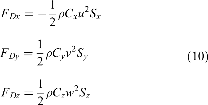
The six degrees of freedom the ducted fan UAV model has 12 states when Euler angles are used to parameterize attitude. The model can be generated in the form of Poincare’s equation in this case¹⁸

\dot{q} = V (q) p

M (q) \dot{p} + C (q, p) p + F (p, q, u) = 0

where q = (ϕ, θ, ψ, x, y, z) ^T , p = (p, q, r, u, v, w) ^T , V (q), M (q), C (q, p), and F (p, q, u) are the kinematic matrix, inertial matrix, gyroscopic matrix, and force function, respectively. The force function contains the aerodynamic, gravitational force, momentum, and so on

\begin{matrix} V (q) = [\begin{matrix} 1 & 0 & 0 & 0 & 0 & 0 \\ S_{θ} T_{θ} & C_{ϕ} & S_{ϕ} C_{θ}^{- 1} & 0 & 0 & 0 \\ C_{ϕ} T_{θ} & - S_{ψ} & C_{ψ} C_{θ}^{- 1} & 0 & 0 & 0 \\ 0 & 0 & 0 & C_{θ} C_{ψ} & C_{θ} S_{ψ} & - S_{θ} \\ 0 & 0 & 0 & S_{ϕ} S_{θ} C_{ψ} - C_{ϕ} S_{ψ} & S_{ϕ} S_{θ} S_{ψ} + C_{ϕ} S_{ψ} & S_{ϕ} C_{θ} \\ 0 & 0 & 0 & C_{ϕ} S_{θ} C_{ψ} + S_{ϕ} S_{ψ} & C_{ϕ} S_{θ} S_{ψ} - S_{ϕ} C_{ψ} & C_{ϕ} C_{θ} \end{matrix}] F (p, q, u) = [\begin{matrix} - \sum M_{x} \\ - \sum M_{y} \\ - \sum M_{z} \\ - \sum F_{x} + g m S_{θ} \\ - \sum F_{y} - g m C_{θ} S_{ψ} \\ - \sum F_{z} - g m C_{θ} S_{ψ} \end{matrix}] \\ C (q, p) = [\begin{matrix} 0 & - I_{y} r & I_{z} q & 0 & - m w & m v \\ I_{x} r & 0 & - I_{z} p & m w & 0 & - m u \\ - I_{x} q & I_{y} p & 0 & - m v & m u & 0 \\ 0 & 0 & 0 & 0 & - m r & m q \\ 0 & 0 & 0 & m r & 0 & - m p \\ 0 & 0 & 0 & - m q & m p & 0 \end{matrix}] M (q) = [\begin{matrix} I_{x} & 0 & 0 & 0 & 0 & 0 \\ 0 & I_{y} & 0 & 0 & 0 & 0 \\ 0 & 0 & I_{z} & 0 & 0 & 0 \\ 0 & 0 & 0 & m & 0 & 0 \\ 0 & 0 & 0 & 0 & m & 0 \\ 0 & 0 & 0 & 0 & 0 & m \end{matrix}] \end{matrix}

where m is the mass of the ducted fan UAVs; g is gravity acceleration; and I_x , I_y , and I_z are the mass moment of inertia. ∑M_x , ∑M_y , ∑M_z , and ∑F_x , ∑F_y , and ∑F_z are total rolling, pitching, yawing moments, and total forces on the aircraft about body axes in x-, y-, and z-axes, respectively. Moreover, C _θ = cos (θ), C ⁻¹ _θ = sec (θ), T_θ = tan (θ), C_ψ = cos (ψ), S _ϕ = sin (ϕ), S _ψ = sin (ψ), C _ϕ = cos (ϕ), and S _θ = sin (θ).

Meanwhile, the proportional-derivative (PD) controller will be used to control the ducted fan UAVs when the hovering state. For the PD controller, the torque at each joint is

T_{i} = k_{p i} (θ_{d i} - θ_{i}) + k_{d i} ({\dot{θ}}_{d i} - {\dot{θ}}_{i}), i = 1, 2

where θ_di is the desired position, k_pi and k_di are the proportional and derivative gains.

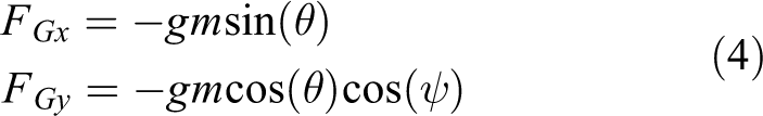
There are several forces and moments: the gravity, lift, control surface, and fuselage acting on the vehicle, respectively.^19
–21

Gravity

Because the roll attitude ϕ and the pitch attitude θ are not zero, the gravity can be decomposed to three forces along the x-, y-, and z-axes

\begin{matrix} F_{G x} = - g m sin (θ) \\ F_{G y} = - g m cos (θ) cos (ψ) \end{matrix}

\begin{matrix} F_{G z} = g m cos (θ) sin (ψ) \\ M_{G x} = M_{G y} = M_{G z} = 0 \end{matrix}

Airfoil

The lift of airfoil can be generated as

\begin{array}{l} F_{B x} = F_{B y} = 0 \\ F_{B z} = - T \end{array}

\begin{array}{l} M_{B x} = M_{B y} = 0 \\ M_{B z} = - M_{e} \end{array}

T = \frac{1}{4} N_{b} (v_{b} - v_{i}) ω_{r} r^{2} ρ a_{0} b c_{r},

v_{b} = v_{i} + \frac{2}{3} ω_{r} r (\frac{3}{4} K_{twist}),

M_{e} = N_{b} \int_{0}^{r} \frac{1}{2} ρ ω_{r} r^{3} C_{D} d r

where v_i represents the induced velocity via the rotor; a_o stand for rotor lift curve coefficient; b denotes the number of the rotor blades; and c_r , ρ, N_b , r, ω_r , k _twist, and C_D are the rotor blade chord, air density, number of airfoil, radius of the rotor, angular velocity, twist of the blades, and drag coefficients of the vehicle, respectively.

Control surface

All of the forces and moments acting on the vehicle by the control surface can be expressed as follows

\begin{matrix} F_{C x} = 2 \frac{1}{2} ρ v_{i}^{2} S_{t} C_{l} (δ_{1}) sin (δ_{1}) \\ F_{C y} = 2 \frac{1}{2} ρ v_{i}^{2} S_{t} C_{l} (δ_{2}) sin (δ_{2}) \\ F_{C z} = 2 \frac{1}{2} ρ v_{i}^{2} S_{t} C_{l} (δ_{1}) sin (δ_{1}) + 2 \frac{1}{2} ρ v_{i}^{2} S_{t} C_{l} (δ_{2}) sin (δ_{2}) + 4 \frac{1}{2} ρ v_{i}^{2} S_{t} C_{l} (δ_{3}) sin (δ_{3}) \end{matrix}

\begin{matrix} M_{C x} = 2 \frac{1}{2} ρ v_{i}^{2} S_{t} C_{l} (δ_{1}) l_{1} \\ M_{C y} = 2 \frac{1}{2} ρ v_{i}^{2} S_{t} C_{l} (δ_{2}) l_{2} \\ M_{C z} = 4 \frac{1}{2} ρ v_{i}^{2} S_{t} C_{l} (δ_{3}) l_{3} \end{matrix}

where δ ₁, δ ₂, and δ ₃ are control vane bias, l ₁, l ₂, and l ₃ are the arms of forces, respectively.

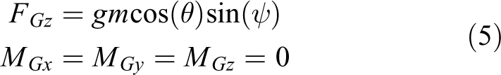
Fuselage

As in the hovering, u = 0, v = 0, w = 0, owing to the fuselage aerodynamic drag, the forces and the moments can be generated as

\begin{matrix} F_{D x} = - \frac{1}{2} ρ C_{x} u^{2} S_{x} \\ F_{D y} = \frac{1}{2} ρ C_{y} v^{2} S_{y} \\ F_{D z} = \frac{1}{2} ρ C_{z} w^{2} S_{z} \end{matrix}

M_{D x} = M_{D y} = M_{D z} = 0

where C_x , C_y , and C_z are the coefficient of lift; S_x , S_y , and S_z are vehicle platform area.

The equations (4) to (11) can be expressed as

\begin{matrix} \sum F_{x} = F_{G x} + F_{B x} + F_{C x} + F_{D x} \\ \sum F_{y} = F_{G y} + F_{B y} + F_{C y} + F_{D y} \\ \sum F_{z} = F_{G z} + F_{B z} + F_{C z} + F_{D z} \end{matrix}

\begin{matrix} \sum M_{x} = M_{G x} + M_{B x} + M_{C x} + M_{D x} \\ \sum M_{y} = M_{G y} + M_{B y} + M_{C y} + M_{D y} \\ \sum M_{z} = M_{G z} + M_{B z} + M_{C z} + M_{D z} \end{matrix}

Combining the kinematics equation (1), dynamics equation (2) with equations (12) and (13) to obtain the state equations

\dot{q} = [\begin{matrix} p + q S_{ϕ} T_{θ} + r C_{ϕ} T_{θ} \\ q C_{ϕ} - r S_{ϕ} \\ q S_{ϕ} C_{θ}^{- 1} + r C_{ϕ} C_{θ}^{- 1} \\ u C_{θ} C_{ψ} + v (S_{θ} S_{ϕ} C_{ψ} - C_{ϕ} S_{ψ}) + w (S_{θ} C_{ϕ} C_{ψ} + S_{ϕ} S_{ψ}) \\ u (C_{θ} S_{ψ}) + v (S_{θ} S_{ϕ} S_{ψ} + C_{ϕ} C_{ψ}) + w (C_{ϕ} S_{θ} S_{ψ} - S_{ϕ} C_{ψ}) \\ - u S_{θ} + v S_{ϕ} C_{θ} + w C_{ϕ} C_{θ} \end{matrix}]

\dot{p} = [\begin{matrix} (\sum M_{x} - q r (I_{z} - I_{y})) / I_{x} \\ (\sum M_{y} - r p (I_{x} - I_{z})) / I_{y} \\ (\sum M_{z} - p q (I_{y} - I_{x})) / I_{z} \\ - (q w - r v) + \frac{1}{m} \sum F_{x} \\ - (r u - p w) + \frac{1}{m} \sum F_{y} \\ - (p v - q u) + \frac{1}{m} \sum F_{z} \end{matrix}]

Numerical calculation of LEs

When equation (14) is combined with equation (15), the nonlinear equations of the ducted fan UAVs can be written as

\dot{X} = f (X)

where X = [q, p] ^T = (ϕ, θ, ψ, x, y, z, p, q, r, u, v, w) ^T is state variable.

The calculation of LEs based on dynamics equation can be written as

λ = lim_{n \to \infty} \frac{1}{n} \sum_{i = 0}^{n - 1} ln {| \frac{d f (X)}{d X} |}_{X_{i}}

To calculate LEs spectrum λ ₁, λ ₂,…, λ ₆. Letting time T is equivalent to 0.01 s and iterations k is equivalent to 100. With regard to k ^th iteration (k = 1, 2,…, k), the initial conditions of the variation equation (16) is set to {v ₁ ^(k−1), v ₂ ^(k−1),…, v ₆ ^(k−1)}. The {v ₁ ^(k−1), v ₂ ^(k−1),…, v ₆ ^(k−1)} is translated into {w ₁ ^(k−1), w ₂ ^(k−1),…, w ₆ ^(k−1)} after the T_s integration. Then, the {w ₁ ^(k−1), w ₂ ^(k−1),…, w ₆ ^(k−1)} is converted into {u ₁ ^(k−1), u ₂ ^(k−1),…, u ₆ ^(k−1)} through the Gram–Schm-orthogonal, the ultimate vector value are the {u ₁ ^k , u ₂ ^k ,…, u ₆ ^k }. Repeat this process and the k chosen large enough.⁵

LEs theory can be applied to build the quantitative relationship between the dynamics stability of the whole system and mechanical–structure parameters shown in Figure 2.

Figure 2.

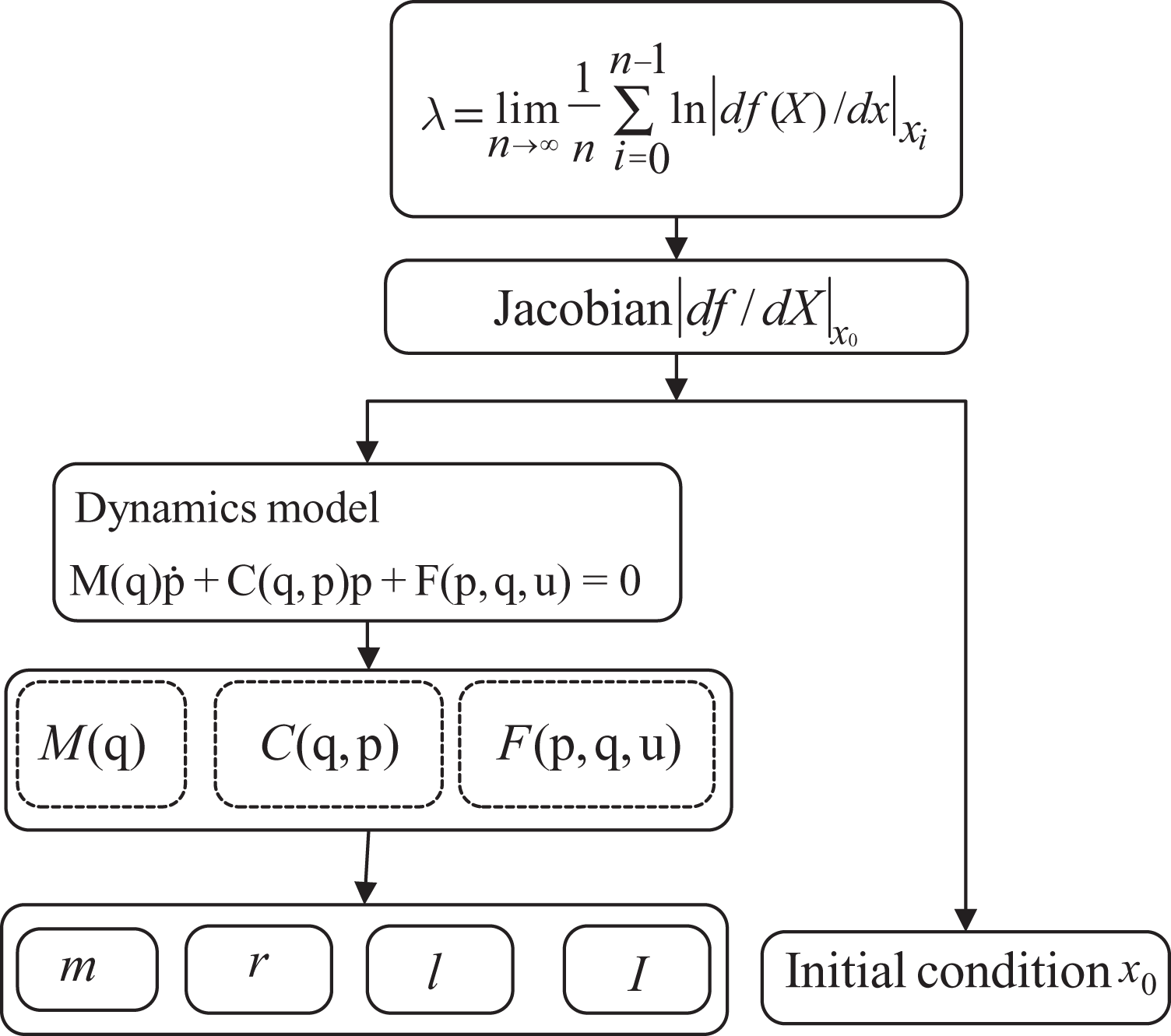
Between Lyapunov exponents and structural parameters.

Simulation results

Parameter identification

To obtain numerical dynamics polynomial of the ducted fan UAVs, m, g, I_x , I_y , I_z , a_o , b, N_b and so on need to be acquired. Here, mechanical–structure parameters of the vehicle existed in Table 1. In simulation analysis, the Mathematica software is used to develop the dynamics model for the ducted fan UAVs during takeoff, landing, and hovering stage, respectively.

Table 1.

The value of mechanical–structure parameters of the system.

Parameters	Value
m	15.5 kg
g	9.8 m/s²
I_x , I_y , I_z	2.374, 2.374, 0.8437 kg m²
a_o	5.9
b	5
N_b	1
r	0.4 m
ω_r	500 r/min
v_i	20 m/s
C_x , C_y _, C_z	0.5, 0.5, 0.1
l _1, l _2, l ₃	0.26, 0.26, 0.55 m
k _wist	0.2618
C_r	0.025 m
A	0.5024 m²
C _l	0.12
C_D	0.5
ρ	1.29 kg/m²

Takeoff stage

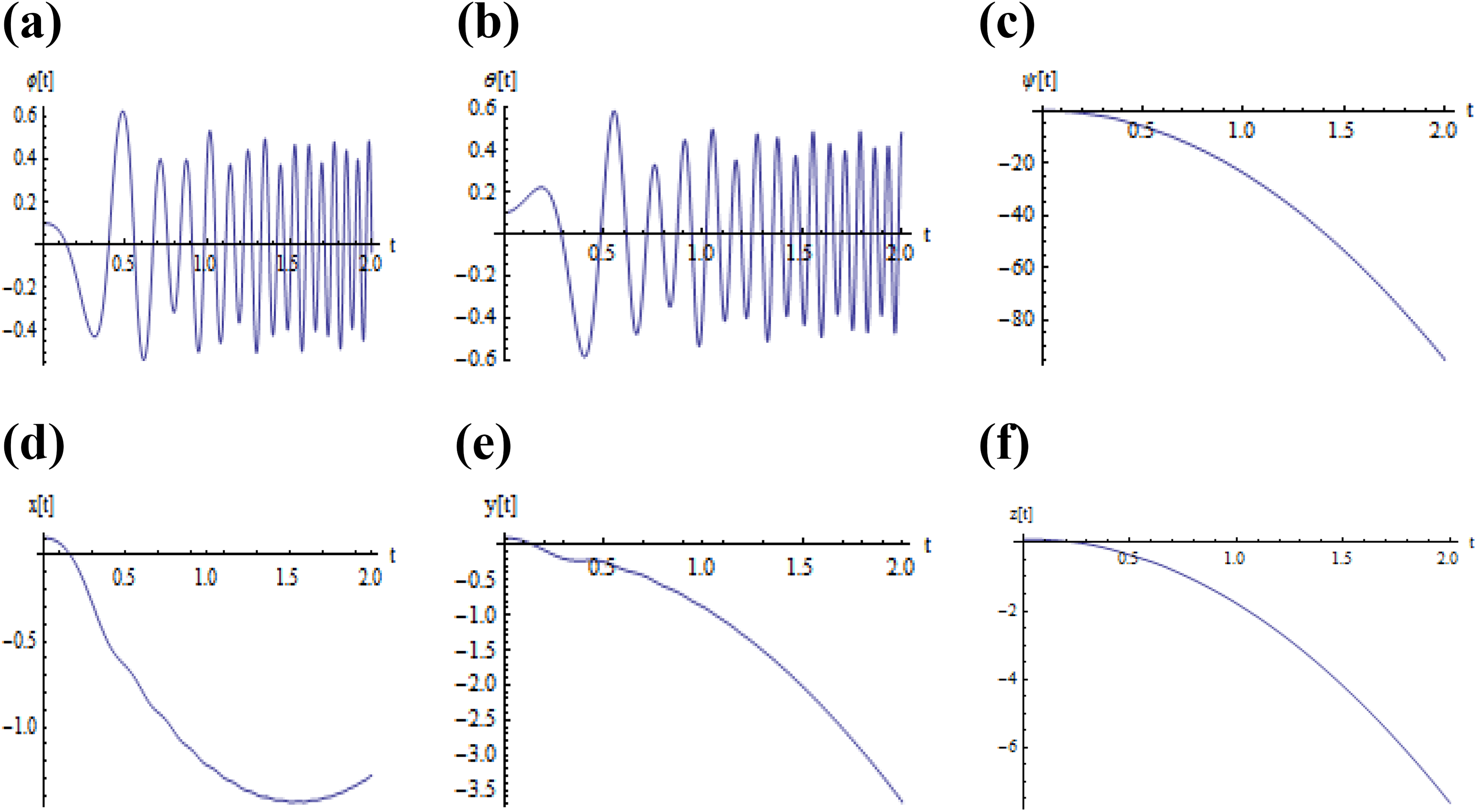
With the propeller speed increased slowly, when the total tensile force in the z-axis is larger than its gravity, the ducted fan UAVs display takeoff state. It can been shown that the attitude of the curve y (t), z (t) display raise, and x (t) displays decline, which is shown in Figure 3.

Figure 3.

The curve of attitude at takeoff state. (a) ϕ (t), (b) θ(t), (c) ψ(t), (d) x (t), (e) y (t), and (f) z(t).

Landing stage

When the speed of rotor of the vehicle decreases, the system emerges landing state, as shown in Figure 4. The curve x (t), y (t), and z (t) will be decreasing.

Figure 4.

The curve of attitude at landing state. (a) ϕ (t), (b) θ (t), (c) ψ (t), (d) x (t), (e) y (t), and (f) z (t).

Seen from Figures 5 and 6, it can be drawn that the convergence rate of the LEs spectrum to zero or negative during the landing stage is much faster than that of takeoff stage, which shows that the dynamic stability of the ducted fan UAVs at landing state is better than at takeoff. It can be used to interpret as the stable aircraft can land even when the engines have no power, only control surfaces are also enough for landing.

Figure 5.

Lyapunov exponents spectrum during takeoff state. (a) λ (ϕ), (b) λ (θ), (c) λ (ψ), (d) λ (x), (e) λ (y), and (f) λ (z).

Figure 6.

Lyapunov exponents spectrum during landing stage. (a) λ (ϕ), (b) λ (θ), (c) λ (ψ), (d) λ (x), (e) λ (y), and (f) λ (z).

For the parametric diversity, based on the mechanical–structural stability analysis, significant insights into the effects of the radius of rotor on the system have been studied. Other mechanical–structure parameters are not unchanged and the value of the rotor radius r is enhanced to 0.6 m (the modified value r is equivalent to 0.6 m, and the original value is equivalent to 0.4 m). Modified the curve of attitude and LEs spectrum shown in Figures 7 and 8, respectively. Looking from Figure 7, it has been revealed that the attitude of the curve x (t), y (t), and z (t) will be greatly decreased compared with Figure 5. Compared with Figures 6 and 8, it can be discover that the value of LEs spectrum at the modified landing state to negative values are larger than during the original landing state. Therefore, changing mechanical–structure parameters can be used to improve its dynamics stability.

Figure 7.

Modified the curve of attitude at landing state. (a) ϕ (t), (b) θ (t), (c) ψ (t), (d) x (t), (e) y (t), and (f) z (t).

Figure 8.

Modified Lyapunov exponents spectrum during landing stage. (a) λ (ϕ), (b) λ (θ), (c) λ (ψ), (d) λ (x), (e) λ (y), and (f) λ (z).

Hovering stage

In this section, by setting the θ_d ₁ = ϕ = 0.7sin(2ϕ), θ_d ₂ = θ = 0.7sin(2θ), and θ_d ₃ = ψ = 0.7sin(2ψ), the controller gains were chosen as the k_p ₁ = 170 (N/rad), k_d ₁ = 40 (NS/rad); k_p ₂ = 90 (N/rad), k_d ₂ = 10 (NS/rad); and k_p ₃ = 110 (N/rad), k_d ₃ = 10 (NS/rad) in the simulations. Figure 10(a) to (c) reveals that the three LEs take about 40 s converge to negative values, indicating the system has been successfully driven to the steady state. Therefore, the controller gain are reasonable. Figure 9(a) to (c) shows that the attitude of the curve ϕ (t), θ (t), and ψ (t) maintains the level trajectory (the angle is approximately equal to 0) after around 3 s (the dash lines are the desired trajectories and the solid lines are the actual trajectories).

Figure 9.

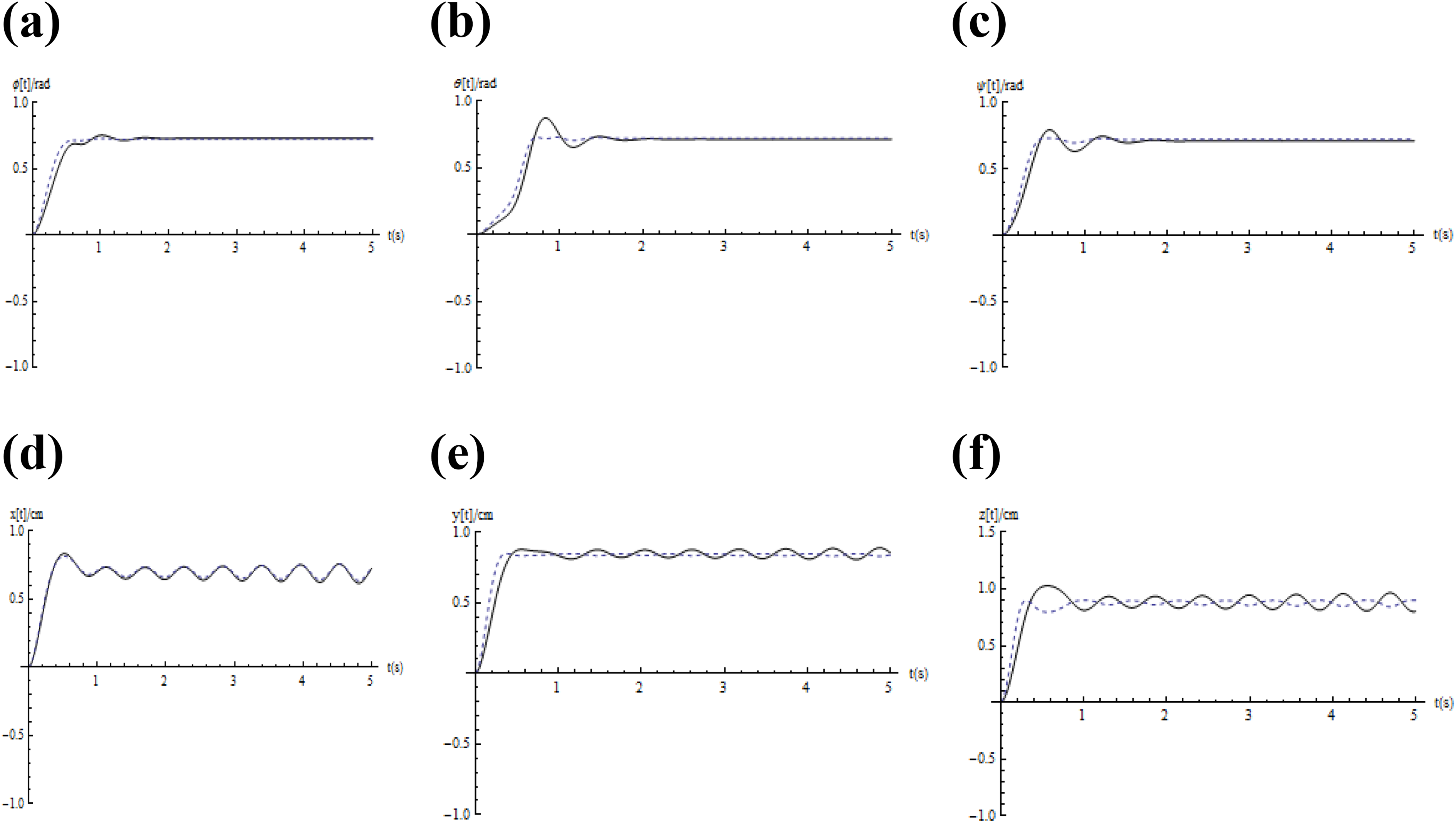
The curve of attitude at hovering state. (a) ϕ (t), (b) θ (t), (c) ψ (t), (d) x (t), (e) y (t), and (f) z (t).

Figure 10.

Lyapunov exponents spectrum during hovering state. (a) λ (ϕ), (b) λ (θ), (c) λ (ψ), (d) λ (x), (e) λ (y), and (f) λ (z).

Meanwhile, letting the θ_d ₄ = x = 1.7sin (2x), θ_d ₅ = y = 1.7sin (2y), and θ_d ₆ = z = 1.7sin (2z); also, the controller gains are selected as k_p ₄ = 1 (N/rad), k_d ₄ = 300(NS/rad); k_p ₅ = 2 (N/rad), k_d ₅ = 350 (NS/rad); and k_p ₆ = 2 (N/rad), k_d ₆ = 250 (NS/rad), it has been shown that all of LEs are negative values, suggesting the system is stable, as shown in Figure 10(d) to (f). Figure 9(d) to (f) also shows that the linear displacement can successfully keep the horizontal trajectory (the linear displacement is approximately equal to 0). On the above analysis in this section point that LE spectrum takes to converge to 0 or negative values, suggesting that the system has been successfully driven to the steady state.

The initial angular displacement was changed into 10⁻¹ (rad) with the same initial angular velocities p, q, and r are equivalent to 0. The results of the attractor are not changed significantly, which demonstrates that the system is not sensitive to the initial condition. This result denotes the system is stable, as shown in Figure 11(a) to (c) (the red line is original stage, and the blue line is modified initial angular displacement).

Figure 11.

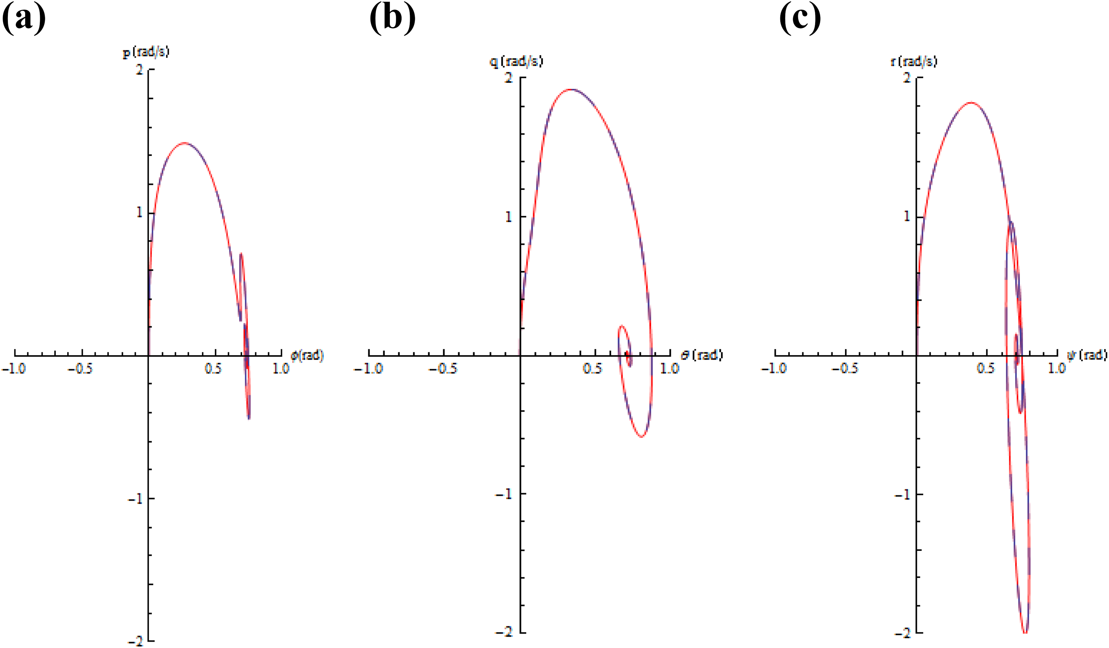
Attractor of the state space. (a) (ϕ-p), (b) (θ-q), and (c) (ψ-r).

Experimental results

In this section, the simulation results of different stages are revealed. The ducted fan UAV’s flight experience is used to Pixhawk’s flight control development environment, as shown in Figure 12, where it can monitor the flight status of the aircraft, data storage, and so on. When the value of rotor radius r is equivalent to 0.6 m, the dynamics stability of the vehicle is much better than that of r is equivalent to 0.4 m in the case of the landing state.

Figure 12.

Online interface of the Pixhawk’s flight control development environment.

Figures 13 to 15 are derived from the online interface of the Pixhawk’s flight control and Figures 16 to 18 are linear displacement parameters in x-, y-, and z-axes, respectively It can be easily observed that the attitude angle of the ducted fan UAVs shows much better convergence to 0 in the value of rotor radius r which is equivalent to 0.6 m than that of r which is equivalent to 0.4 m according to Figures 16 to 18 in landing stage. This conclusion can be used to verify the compared results of Figure 6 with Figure 8. The ducted fan UAV’s stability in landing is better than in takeoff according to the comparison of Figures 4 and 6. Figures 19 to 21 are also obtained from the online interface of the Pixhawk’s flight control development environment of the ducted fan UAV, which show the three Eluer angular of the system in x-, y-, and z-axes, respectively. The experimental results show that the ducted fan UAV has much better flight performance in the landing stage than in the takeoff stage, which can be proved in the results of Figures 4 and 6. Figures 19 to 21(a) show that the attitude of the roll, pitch, and yaw maintain the level trajectory (the angle is approximately equal to 0) over time than Figures 19 to 21(b). In summary, the optimization of mechanical–structure parameters can be used to promote dynamics stability.

Figure 13.

Experimental attitude of the curve location parameter of in the x-axis during landing state. (a) r = 0.4 m and (b) r = 0.6 m.

Figure 14.

Experimental attitude of the curve location parameter of in the y-axis during landing state. (a) r = 0.4 m and (b) r = 0.6 m.

Figure 15.

Experimental attitude of the curve location parameter of in the z-axis during landing state. (a) r = 0.4 m and (b) r = 0.6 m.

Figure 16.

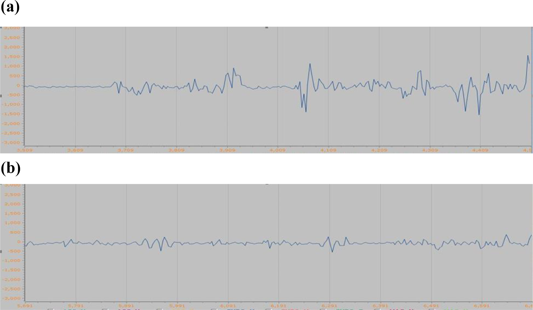
Experimental attitude of the curve angular in the x-axis during landing state. (a) r = 0.4 m and (b) r = 0.6 m.

Figure 17.

Experimental attitude of the curve angular in the y-axis during landing state. (a) r = 0.4 m and (b) r = 0.6 m.

Figure 18.

Experimental attitude of the curve angular in the z-axis during landing state. (a) r = 0.4 m and (b) r = 0.6 m.

Figure 19.

The curve angular in the x-axis. (a) Roll angular during takeoff stage and (b) roll angular during landing stage.

Figure 20.

The curve angular in the y-axis. (a) Pitch angular during takeoff stage and (b) pitch angular during landing stage.

Figure 21.

The curve angular in the y-axis. (a) Yaw angular during takeoff stage and (b) yaw angular during landing stage.

Conclusions

The stability analysis is very important for the development of the ducted fan UAVs. This article has proposed to use the concept of LEs to establish the quantification relationship between the ducted fan UAV’s structural parameters and its motion stability to optimize structural parameters for increased dynamics stability. This concept is one of the most powerful tools for analyzing complex nonlinear dynamical system. Furthermore, LEs are “invariant” measures of dynamics characteristics, that is, independent of the initial condition. However, existing methods are either not constructed, for example, Lyapunov’s second methods, or sensitive to the individual testing or initial conditions, such as simulation-based methods. The proposed method via the concept of LEs is constructive and theoretically sound in this article, owing to the exponents are “invariant” measures of system dynamics.

Three different stage of stability, such as takeoff, landing, and hovering stage, respectively, have been rigorously analyzed in this article using the concept of LEs for the ducted fan UAVs. In the case of landing stage stability analysis, the radius range of rotor where the vehicle stability is guaranteed has been changed. It has shown significant insights into the effects of mechanical–structure parameters on dynamics stability. Moreover, the state space is another important property of a dynamics system. To investigate the effect of the initial condition on state space. The PD controller has been presented for the hovering state. The disturbance of system stability comes from initial conditions. It can be derived that the vehicle is stable and will return to its stable fixed point, which verifies the stable under the suitable PD controller. The conclusion is the optimization of mechanical–structure parameters has exerted significant effects on its stability.

The main contribution of this article lies in the fact that it starts from symbol dynamic modeling to stability analysis using the concept of LEs. The optimization of structure parameters is of great significance to improve the movement stability of the ducted fan UAVs. Therefore, this article builds the quantitative relationship between the structural parameter of the ducted fan aerial vehicles and their system stability based on LEs theory from viewpoint of structural parameters design. Moreover, the reliability and stability of ducted fan UAVs under service could be promoted by optimizing the mechanical–structure parameters.

As discussed earlier, the presented method for calculating LEs is applicable to general dynamics systems provided that the mathematical models are available. Therefore, the proposed method can be extended to more complex models, especially to multi-body dynamics system, which is the subject of future work.

Footnotes

Acknowledgements

We thank the anonymous reviewers for helpful and insightful remarks. In addition, I want to thank, in particular, the patience, care, and support from XX Chen over the passed years.

Declaration of conflicting interests

The author(s) declared no potential conflicts of interest with respect to the research, authorship, and/or publication of this article.

Funding

The author(s) disclosed receipt of the following financial support for the research, authorship, and/or publication of this article: This research is supported by the National Key Research and Development Plan, the On-line monitoring technology and equipment of contact acoustic flow (Grant No. 2017YFC0405702), and central public welfare basic scientific research institutes special funds (Grant No. Y919008).

ORCID iD

Cheng Chen

References

Chang

Bang

Lee

et al. Dynamic modeling and fuzzy control for a small tiltrotor unmanned aerial vehicle. Int J Adv Robot Syst 2012; 227(9): 1468–1487.

Amiri

Ramirez-Serrano

Davies

. Integral back stepping control of an unconventional dual-fan unmanned aerial vehicle. J Intell Robot Syst 2013; 69: 147–159.

Corsini

Rispoli

Sheard

. Computational analysis of noise reduction devices in axial fans with stabilized finite element formulations. Comput Mech 2012; 50: 695–705.

Wang

Chen

Guo

. Numerical analysis of aerodynamic characteristics for the design of a small ducted fan aircraft. J Aeros Eng 2012; 227(10): 1556–1570.

Shin

Shon

et al. Indoor hovering control of small ducted fan type OAV using ultrasonic positioning system. J Intell Robot Syst 2011; 61: 15–27.

Liu

Wang

. Quantitative stability of quadrotor unmanned aerial vehicles. Nonlinear Dyn 2017; 87: 1819–1833.

Wadduwage

Annakkage

. Power system transient stability analysis via the concept of Lyapunov exponents. Electr Pow Syst Res 2013; 104: 183–192.

Liu

Chen

et al. Structural stability analysis and optimization of the quadrotor unmanned serial vehicle via the concept of Lyapunov exponents. Int J Adv Manuf Technol 2016; 85(5–8): 1–11.

Sekhavat

Sepehri

. Calculation of Lyapunov exponents using nonstandard finite difference discretization scheme: a case study. J Differ Equ Appl 2004; 10(4): 369–378.

10.

Sadri

. Modified Lyapunov exponent, new measure of dynamics. Nonlinear Dyn 2014; 78: 2731–2750.

11.

Yang

. On stability analysis via Lyapunov exponents calculated from a time series using nonlinear mapping a case study. Nonlinear Dyn 2010; 59: 239–257.

12.

Sun

. Stability analysis via the concept of Lyapunov exponents: a case study in optimal controlled biped standing. Int J Control 2012; 85(12): 1952–1966.

13.

Omar

Ghada

Abderrazak

. Global stabilization of an adaptive observer-based controller design applied to induction machine. Int J Adv Manuf Technol 2015; 81: 423–432.

14.

Zevin

Pinsky

. Absolute stability criteria fora generalized Lur’e problem with delay in the feedback. Siam J Control Optimal 2005; 43(6): 2000–2008.

15.

Amy

Balling

. Structural analysis and optimization of tall buildings connected with sky bridges and atria. Struct Multidisc Optim 2017; 55: 583–600.

16.

Miha

Kosel

Drazumeric

. Structural optimization using global stress-deviation objective function via the level-set method. Struct Multidisc Optim 2017; 55: 91–104.

17.

Daniel

. Comprehensive system identification of ducted fan UAV. San Luis Obispo: California Polytechnic State University, 2004, pp. 17–52.

18.

Liu

Huang

Wang

et al. Nonlinear dynamics modeling and simulation of two-wheeled self-balancing vehicle. Int J Adv Robot Syst 2016; 13(6): 1–9.

19.

Johnson

Turbe

. Modeling, control, and flight testing of a small ducted fan aircraft. J Guid Control Dynam 2006; 29(4): 769–779.

20.

Wang

et al. Modeling, control and flight testing for a saucer ducted fan UAV. In: 2010 3rd international symposium on systems and control in aeronautics and astronautics, Harbin, 2010, pp. 930–935. DOI: 10.1109/ISSCAA.2010.5633048.

21.

Martini

Léonard

Abba

. Dynamic modelling and stability analysis of model-scale helicopters under wind gust. J Intell Robot Syst 2009; 54: 647–686.

On dynamic characteristics and stability analysis of the ducted fan unmanned aerial vehicles

Abstract

Keywords

Introduction

Methodology

Dynamic analysis and modeling

Gravity

Airfoil

Control surface

Fuselage

Numerical calculation of LEs

Simulation results

Parameter identification

Takeoff stage

Landing stage

Hovering stage

Experimental results

Conclusions

Footnotes

Acknowledgements

Declaration of conflicting interests

Funding

ORCID iD

References