Trajectory tracking control of an amphibian robot with operational capability

Abstract

Although the traditional amphibious robot has the ability of multi-space motion, it has the disadvantage of low power utilization and no operational capability. In order to make it competent in an extremely complex environment, we studied the structural design and control of amphibian robot with operational capability. First, in order to make the robot have the ability of flying in the sky, moving on land, and swimming in the water, a “bevel variant” mechanism for power switching is designed. Then, taking the uncertainty of the kinetic parameters and external influences into account, the kinetic and kinematic models of the system are established. Next, a sliding mode controller that outputs control force for the system and a quadratic calculation optimization algorithm for inverse kinematics solution are designed. Finally, the simulation platform for the system is built based on MATLAB. The simulation results show that when the system is in the land and air flight stages, the vehicle position and orientation tracking error are within ±0.05 m and ±2°, respectively. When the system is in the underwater stage, the end effector position and orientation tracking error are within ±0.15 m and ±3.0°, respectively.

Introduction

On June 23, 2018, 12 junior football players and a coach from Thailand entered a cave to explore in Chiang Rai. The cave was then flooded by rain and they lost contact with the outside world. Under the nonstop rescue of professional rescue teams from all over the world, the trapped people were finally rescued. However, the rescue operation was extremely resistant, and the arduousness far exceeded the rescue expectations. After a full 9 days of rescue, the exact position of the football team was determined. The main reason for the slow rescue is that the terrain in the cave is extremely complicated. The narrowest part of the tunnel is only 70 cm. Some sections of the tunnel are even completely submerged by water, and the underground passage is filled with sediment, gravel, and various debris. In this closed, dark, and complex deep hole space, if the rescue diver unfortunately runs out of oxygen, loses illumination, and loses the direction of the hole in the search and rescue process, the consequences will be unimaginable. Not only the rescue situation, the problem will also occur in the scenes of investigation, maintenance, and so on. Therefore, it is very useful to design an amphibious robot with stable performance and different space motion capabilities.

However, for amphibious robots, whether the robots have a flexible and efficient driving module is the main limiting factor for its practical application. The current drive module of amphibian robot is either a simple power superposition using wheel–rotor–propeller or a mechanism for vector propulsion. ^1,2 The simple power superposition method has problems such as low power utilization, power idle, and increased body weight. The mechanism-based vector propulsion method results in a larger drive module due to its complicated transmission, and the propeller has less swinging posture and smaller swinging space. Not only that, amphibious robots often require four or six sets of vector propulsion device to meet the requirements of multi-space motion. Taking the vector propulsion device based on space link-universal joints proposed by Michelini as an example, if calculated by six sets of the device, only the driving part of the robot requires up to 24 motors. ³ Therefore, if a simple and reliable variant propulsion mechanism can be designed for an amphibious robot, it can not only simplify the structure of the robot, but also effectively reduce the complexity of the control algorithm.

To be applied to complex environments such as caves and mines, robots need to have the enhanced operational ability. Therefore, it is necessary to equip the robot with multi-degree of freedom manipulator to make up an amphibious variant vehicle-manipulator system (AVVMS). However, due to the coupling between the vehicle and the manipulator, the disturbance of the external environment such as ocean current/wind and the uncertainty of the hydrodynamic parameters, it is difficult for controller to coordinate the movement between the vehicle and the manipulator appropriately. Chen et al. simplified the design of the control system by simplifying the kinematics and dynamics equations of the vehicle-manipulator system, but the accuracy of the simulation results is also reduced. ⁴ Mohan and Kim designed an adaptive coordinated controller based on Kalman filter, but the controller relies on the accuracy of the filter. ⁵ Antonelli et al. used the sliding mode control as the dynamic controller to control the underwater vehicle-manipulator system, but ignored the non-matching of ocean currents and the coupling of motion. ^{6 –12} Zhang et al. used the weighted minimum norm method to avoid joints reaching the angular limit position and the interference between the vehicle and the manipulator, but the tracking error of the end effector increases with time. ^13,14

Based on the above problems, we first propose a “bevel variant” mechanism for power switching. This mechanism has the advantages of stable switching, small occupation, and high energy utilization, and can better meet the multi-motion shape requirements of hobby robots. Then, the kinetic and kinematic models of AVVMS were established after comprehensively considering the uncertainty of the kinetic parameters and the external interference. Finally, the inverse kinematics controller based on the quadratic computational optimization algorithm is combined with the sliding mode controller that controls the dynamics of the system to obtain the overall motion control scheme of AVVMS. The simulation results show that the AVVMS has good trajectory tracking ability under the control of this scheme, and the end manipulator has higher positioning accuracy when performing tasks.

Structure design idea and implementation plan of AVVMS

Figure 1(a) is the schematic diagram of AVVMS, it consists of four modules: vehicle, drive device, “bevel variant” mechanism, and a multi-degree of freedom manipulator. Among them, the principle of “bevel variant” mechanism is: a rotating pair is formed between the chassis of the drive device and the bracket end face, and the rotating pair can be rotated 360° around the central axis; the bracket end face is at an angle to the ground level and is a fixed bevel; the chassis surface of the drive device is a rotatable bevel, adjusting the angle between the bevel and the bevel of the bracket will change the attitude of the propeller; when applied, the rotation angle value can be reasonably controlled, and the propulsion direction of the propeller can be changed. The “bevel variant” mechanism subtly utilizes the principle of the bevel attitude transformation. The power source after switching to the appropriate attitude can meet the requirements of the current environment. Compared with the method of simple power superposition or the mechanism-based vector propulsion, the method can not only simplify the structure of the robot, but also effectively reduce the complexity of the control algorithm.

Figure 1.

The schematic of AVVMS in different motion states. (a) Composition of AVVMS, (b) flying in the air by six rotors, (c) driving on land by six wheels, and (d) sailing in the water by six propellers. AVVMS: amphibious variant vehicle-manipulator system.

AVVMS has three motion modes. As shown in Figure 1(b), the drive device can be converted into a horizontal state by rotating the “bevel variant” mechanism, which can become an aerial vehicle-manipulator system. As shown in Figure 1(c), the drive device can be converted into a land-wheeled state. At this time, the robot is no longer driven by the propeller, but by the wheels. As shown in Figure 1(d), the underwater vehicle-manipulator system is also driven by propeller, but the specific angle of the “bevel variant” mechanism can be changed in real time according to the underwater tasks. For example, when the robot dive and ascend, the pose of the six propellers will be adjusted to a horizontal state. Because in this state, the efficiency of the propeller can be fully utilized.

Kinematics and dynamics modeling of AVVMS

Kinematic modeling

The model and the coordinate frame arrangement of AVVMS are shown in Figure 2. Σ_I is the inertial frame, Σ_b is the vehicle frame, Σ_i is the joint frame, and Σ_e is the end effector frame. The kinematic equation of AVVMS can be expressed as follows

$\dot{\xi }=J_{a,s}\zeta$

1

Figure 2.

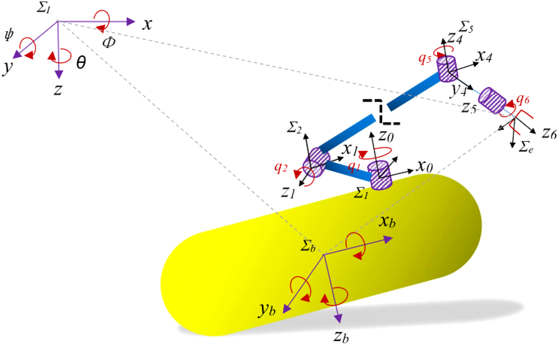
AVVMS with its coordinate frame arrangement. AVVMS: amphibious variant vehicle-manipulator system.

where $\xi ={\left[\mathrm{\eta }q\right]}^{\text{T}}$ is the vector of absolute positions, Euler angles and the manipulator joint angles of AVVMS; $\eta ={\left[xyz\varphi \theta \psi \right]}^{\text{T}}$ is the absolute positions, Euler angles of the vehicle, x-surge position, y-sway position, z-heave position, ϕ-roll angle, θ-pitch angle, ψ-yaw angle, respectively; q_i is the joint position of the link i. The velocity of AVVMS in the vehicle frame is $\zeta ={[v\dot{q}]}^{\text{T}}$ , where $v={\left[uvwpqr\right]}^{\text{T}}$ , u, v, w representing the linear velocity of x, y, z, respectively; p, q, r representing the angular velocity of roll, pitch, and yaw, respectively; J_a,s is the Jacobian matrix of the system velocity converted to the inertial frame velocity.

The tasks are often accomplished by the end effector, so the states of the end effector need to be considered. The velocity of the joint frame Σ_i with respect to the inertial frame Σ_I is expressed as

$V_{oi}=J_{io}\zeta =\left[A{d}_{g_{bi}}^{-1}A{d}_{g_{bi}}^{-1}{J}_i\right]\zeta$

2

Let i = e in equation (2) to get the end effector velocity with respect to the inertial frame

$V_{oe}=J_{eo}\zeta =\left[A{d}_{g_{be}}^{-1}A{d}_{g_{be}}^{-1}{J}_n\right]\zeta$

3

The AVVMS is inevitably subjected to ocean current or wind when moving under water or in the air. However, most controllers directly ignore the interference or consider the ocean current or wind interference as constant disturbance.

Let us assume that the ocean current or wind velocity, expressed in the inertial frame, ${\nu }_c^I$ is constant and irrotational. It can be represented as

$v_c^I=\left[\begin{array}{c}{\nu }_{cx}\\ {\nu }_{cy}\\ {\nu }_{cz}\\ 0\\ 0\\ 0\end{array}\right]$

4

Current or wind effects can be added to the dynamic of a rigid body moving in a fluid simply considering the relative velocity in vehicle frame in the derivation of the Coriolis and centripetal terms and the damping terms. After considering the disturbance, the total velocity relative to the current can be described as follows

${\zeta }_r=\zeta -\text{blockdiag }\{R_I^B,O\}{v}_c^I$

5

Defined $H_m\left(\xi \right)={\left[\begin{array}{cc}{R}_I^B& 0_{9\times 3}\end{array}\right]}^{\text{ T}}$ and $H_n\left(\xi ,\zeta \right)={\left[\begin{array}{cc}-R_I^B{\widehat{\omega }}_{ob}& 0_{9\times 3}\end{array}\right]}^{\text{ T}}$ , equation (5) can be written as

${\zeta }_r=\zeta -H_m\left(\xi \right){\upsilon }_c^o$

6

while the relative acceleration yields

${\dot{\zeta }}_r=\dot{\zeta }-H_n\left(\xi ,\zeta \right){\upsilon }_c^o$

7

where R_ob is the matrix representing the rotation of Σ_b with respect to Σ_I and ω_ob is the rotational velocity of vehicle as observed from vehicle frame Σ_b .

Dynamic modeling

By using the Newton–Euler and recursive Newton–Euler formulations, the dynamic equations in the inertial frame of an AVVMS can be expressed as follows ^{6,15 –18}

$$\begin{gathered} M_{RB}(\xi )\dot{\zeta }+C_{RB}(\xi ,\zeta )\zeta +M_A(\xi ){\dot{\zeta }}_r+C_A(\xi ,{\zeta }_r){\zeta }_r \\ +D(\xi ,{\zeta }_r){\zeta }_r+N\left(\xi \right)={\tau }_c \end{gathered}$$

8

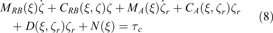
From equations (6) and (7), we have that ${\zeta }_r=\zeta -H_m\left(\xi \right){\upsilon }_c^o$ and ${\dot{\zeta }}_r=\dot{\zeta }-H_n\left(\xi ,\zeta \right){\upsilon }_c^o$ . We can then write equation (8) in a more compact way as

$M(\xi )\dot{\zeta }+C(\xi ,\zeta ,{\zeta }_r)\zeta +D(\xi ,{\zeta }_r)\zeta +N\left(\xi \right)+\Pi (\xi ,\zeta ,{\zeta }_r)={\tau }_c$

9

where $M(\xi )=M_{RB}(\xi )+M_A(\xi ),C(\xi ,\zeta ,{\zeta }_r)=C_{RB}(\xi ,\zeta )+C_A(\xi ,{\zeta }_r),\Pi (\xi ,\zeta ,{\zeta }_r)=M_A(\xi )H_n(\xi ,\zeta )-(C_A(\xi ,{\zeta }_r)+D(\xi ,{\zeta }_r))H_m(\xi )v_c^o,M_{RB}(\xi )\dot{\zeta }$ is the vector of inertial forces and moments of the system. $C_{RB}(\xi ,\zeta )\zeta$ is the vector of Coriolis and centripetal effects of the system. $M(\xi )$ is the inertia matrix of the system (including added mass matrix and interaction/coupling effect inertia matrix). $C(\xi ,{\zeta }_r)$ is the Coriolis and centripetal matrix of the system (including added mass Coriolis and centripetal matrix). $D(\xi ,{\zeta }_r)$ is the damping matrix of the system (both linear and quadratic damping matrix). $N(\xi )$ is the vector of restoring effects of the system (both buoyancy and gravity effects). τ_c is the vector of control inputs of AVVMS. In the land and flight modes, the robot is no longer affected by the water environment. Therefore, the vector of inertial forces and moments $M_A(\xi ){\dot{\zeta }}_r$ , the Coriolis and centripetal $C_A(\xi ,{\zeta }_r){\zeta }_r$ , the viscous force and the moment vector $D(\xi ,{\zeta }_r){\zeta }_r$ are all zero vectors. Apart from this, $N(\xi )$ only needs to consider the effect of gravity without considering the influence of buoyancy.

The control forces of AVVMS is ${\tau }_c={\left[{\tau }_1{\tau }_2{\tau }_3{\tau }_4{\tau }_5{\tau }_6{\tau }_7{\tau }_8{\tau }_9{\tau }_{10}{\tau }_{11}{\tau }_{12}\right]}^{\text{T}}$ , where τ _{1 – 6} is the control forces and torques acting on the vehicle and τ _7–12 is the control torques acting on the joints of the manipulator. Define $u={\left[T_1{T}_2{T}_3{T}_4{T}_5{T}_6\right]}^{\text{T}}$ as the thrust matrix for each propeller and B as the thrust distribution matrix, the forces generated by the propeller in the six degrees of freedom can be expressed as τ _c = Bu.

Coordinated controller design of AVVMS

Figure 3 shows the control scheme of AVVMS. The input reference signal of the control system is the desired velocity of the end effector V _ed , which is given by trajectory planner. According to V_ed and the measured states ξ of the system, the inverse kinematics controller plans the desired states ξ_d , and use ξ_d and ξ together as the input of the sliding mode controller. Then the sliding mode controller outputs the control forces τ _c to the robot to obtain the measured states ξ_d . After the operator has clarified the current environment in which the robot is located, it can be adapted to the current environment by reasonable control of the “bevel variable” mechanism.

Figure 3.

Block diagram representation of the proposed control scheme.

Dynamic control of AVVMS

In this section, the application of a sliding mode-based approach to motion control of AVVMS is discussed.

For the sliding mode controller, the following manifold is used

$s=\zeta -{\zeta }_s$

10

ζ_S is the virtual reference velocity and defined as

${\zeta }_s={\zeta }_d+\Lambda e$

11

where ${\zeta }_d={\left[\begin{array}{ccc}{\upsilon }_d^{\text{ T}}& {\omega }_d^{\text{T}}& {\dot{q}}_d^{\text{T}}\end{array}\right]}^{\text{ T}},e={\left[\begin{array}{ccc}\stackrel{\sim }{x}& \stackrel{\sim }{\epsilon }& \stackrel{\sim }{q}\end{array}\right]}^{\text{T}},\Lambda =\left[\begin{array}{ccc}{K}_p& 0_{3\times 3}& 0_{3\times 6}\\ 0_{3\times 3}& -2c\frac{\partial W}{\partial \eta }{I}_{3\times 3}& 0_{3\times 6}\\ 0_{6\times 3}& 0_{6\times 3}& K_q\end{array}\right]$ .

We now propose the following control input, as follows

${\tau }_c=\stackrel{\wedge }{M}{\dot{\zeta }}_s+\stackrel{\wedge }{C}{\zeta }_s+\stackrel{\wedge }{D}{\zeta }_s+\stackrel{\wedge }{N}+\stackrel{\wedge }{\Pi }-K_{d}s-K_s\text{sign}(s)$

12

where $\widehat{·}$ denotes the estimate of a matrix or vector, and ${\text{sign}}_i(x_i)=\{\begin{array}{c}1\text{ if }{x}_i>0\\ 0\text{ if }{x}_i=0\\ -1\text{ otherwise }\end{array}$ .

Stable analysis

To ensure that the system converges to the sliding manifold s = 0, we use the following Lyapunov candidate functions

$V=\frac{1}{2}{s}^{\text{T}}M\text{ s}$

Taking the time derivative of V and substituting equation (12) into equation (13) yields

$$\begin{gathered} \dot{V}=s^{\text{T}}M\dot{\text{s}}+\frac{1}{2}{s}^{\text{T}}\dot{M}s=s^{\text{T}}({\tau }_c-C{\zeta }_s-D{\zeta }_s-N-\Pi -M{\dot{\zeta }}_s) \\ +\frac{1}{2}{s}^{\text{T}}\text{(}\dot{\text{M}}-\text{2C) }s-s^{\text{T}}Ds \end{gathered}$$

Since the matrix $\dot{M}-2C$ is skew symmetric, then $s^{\text{T}}(\dot{M}-2C)s/2 = 0$ . We can write $\dot{V}$ as

$\dot{V}=s^{\text{T}}({\tau }_c-C{\zeta }_s-D{\zeta }_s-N-\Pi -M{\dot{\zeta }}_s)-s^{\text{T}}Ds$

13

Substituting equation (12) into equation (13) yields

$$\begin{gathered} \dot{V}=-s^{{ }^{\text{T}}}(D+K_d\text{)}s-s^{{ }^{\text{T}}}(\tilde{M}{\dot{\zeta }}_s+\tilde{C}{\zeta }_s+\tilde{D}{\zeta }_s+\tilde{N}+\tilde{\Pi } \\ +K_s\text{sign}(s)) \end{gathered}$$

14

where $\stackrel{\sim }{·}$ denotes the difference between the true value and the estimated value of the parameter, and for simplicity, we define $\stackrel{\sim }{Y}=\tilde{M}{\dot{\zeta }}_s+\tilde{C}{\zeta }_s+\tilde{D}{\zeta }_s+\tilde{N}+\tilde{\Pi }$ . The matrix $D+K_d$ is positive definite, we can get the following upper bound on $\dot{V}:\dot{V}<-{\lambda }_{\text{min}}(K_s)\Vert s\Vert +\Vert \tilde{Y}\Vert \Vert s\Vert$ . By choosing K_s to satisfy ${\lambda }_{\text{min}}(Ks)>\Vert \tilde{Y}\Vert$ , we ensure that $\dot{V}$ is negative definite. Then applying the Lyapunov direct method to nonautonomous systems, the global unified asymptotic stability of s = 0 is obtained.

When the modeling uncertainty or interference is large, it is necessary to set the gain η of the switching term to be large. However, large gain will cause obvious chattering. In order to eliminate chattering, the controller uses the saturation function $\text{sat}\left(s\right)$ instead of $\text{sign}\left(s\right)$ . The function $\text{sat}\left(s\right)$ does not require switching of the control structure on the switching plane. It can be a control system that performs structural transformation on the boundary layer, or a continuous state feedback control system that does not perform structural transformation at all. This difference in the implementation of the quasi-sliding mode control makes it fundamentally avoid or weaken the chatter. The $\text{sat}\left(s\right)$ can be defined as ${\text{sat}}_i(x_i)=\{\begin{array}{l}{\text{sign}}_i\text{(}x\text{) }|{\text{x}}_{\text{i}}\text{/}\epsilon |>1\\ x_i/\epsilon \text{ otherwise}\end{array}$ .

Stability of the sliding manifold

In order to make the stability of the sliding manifold, it is necessary to ensure that the vehicle translational error $\stackrel{\sim }{x}$ , the vehicle rotational error $\stackrel{\sim }{\epsilon }$ , and the manipulator error $\stackrel{\sim }{q}$ converge to zero. For this reason, the stability of s = 0 is now decomposed into three parts: the vehicle translational part, vehicle rotational part, and the manipulator part.

The convergence of the manipulator error $\stackrel{\sim }{q}$ is guaranteed by taking K_q to be positive definite, that is, K_q > 0. Choose $V={\stackrel{\sim }{q}}^{{\rm T}}\stackrel{\sim }{q}/2 > 0$ as the Lyapunov candidate function, and deriving for V yields $\dot{V}={\stackrel{\sim }{q}}^{{\rm T}}\dot{\stackrel{\sim }{q}}={\stackrel{\sim }{q}}^{{\rm T}}$ . Using the Lyapunov direct method, the dynamic error of the manipulator is asymptotically stable.

Rotational error dynamics of the vehicle. Choose $W(\dot{\eta })$ as the Lyapunov candidate function, $\dot{W}\left(\stackrel{\sim }{\eta }\right)=\frac{\partial W}{\partial \stackrel{\sim }{\eta }}\dot{\stackrel{\sim }{\eta }}=-\frac{1}{2}\frac{\partial W}{\partial \stackrel{\sim }{\eta }}{\stackrel{\sim }{\epsilon }}^{{\rm T}}\stackrel{\sim }{\omega }=-c{\left(\frac{\partial W}{\partial \stackrel{\sim }{\eta }}\right)}^2{\stackrel{\sim }{\epsilon }}^{{\rm T}}\stackrel{\sim }{\epsilon }$ . Let $W\left(\stackrel{\sim }{\eta }\right)=1-|\stackrel{\sim }{\eta }|$ , $\partial W/\partial \stackrel{\sim }{\eta }=-sign\left(\stackrel{\sim }{\eta }\right)$ can be obtained. Due to $\tilde{\eta }=\text{ cos}(\beta /2)$ , $|\tilde{\eta }|\le 1$ . The Lyapunov candidate function $W\left(\stackrel{\sim }{\eta }\right)$ is positive except when $\tilde{\eta }=\pm 1$ . When $\tilde{\eta }\ne \pm 1$ , the derivative function $\dot{W}(\stackrel{\sim }{\eta })$ of $W\left(\stackrel{\sim }{\eta }\right)$ is negative and gradually converges to ±1 to reach a stable equilibrium.

Translational error dynamics of the vehicle. Firstly, we define ${\dot{x}}_d=R(Q)v_d$ , which yields $\stackrel{\sim }{v}= R{(Q_d)}^{\text{T}}\dot{\stackrel{\sim }{x}}$ . Then, we define K_P = λR(Q_d )^T, λ > 0. By substituting K_P = λR(Q_d )^T and $\stackrel{\sim }{v}= R{(Q_d)}^{\text{T}}\dot{\stackrel{\sim }{x}}$ into $\stackrel{\sim }{v}=-K_p\stackrel{\sim }{x}$ , we get the following error dynamics for the translational motion of the vehicle on the manifold: $\dot{\stackrel{\sim }{x}}=-\lambda \stackrel{\sim }{R}\stackrel{\sim }{\text{x}}$ , where $\stackrel{\sim }{R}=R(Q)R{(Q_d)}^{\text{T}}$ . The function for calculating the matrix eigenvalues and eigenvectors is $\text{eig}(\stackrel{\sim }{R})\in (\begin{array}{cc}1,& 2{\stackrel{\sim }{\eta }}^2-1\pm j2\stackrel{\sim }{\eta }\sqrt{1-{\stackrel{\sim }{\eta }}^2}\end{array})$ , $\stackrel{\sim }{R}$ is strictly positive for ${\stackrel{\sim }{\eta }}^2>1/2$ . Since $\stackrel{\sim }{\eta }=\text{ cos}(\stackrel{\sim }{\beta }/2)$ , $\stackrel{\sim }{R}$ is strictly positive. Since the rotation error converges uniformly to zero, the positive-definiteness of $\stackrel{\sim }{R}$ will be satisfied after, at least, a transient period, and from $\dot{\stackrel{\sim }{x}}=-\lambda \stackrel{\sim }{R}\stackrel{\sim }{\mathit{\text{x}}}$ , it follows that $\stackrel{\sim }{x}$ converges to zero.

Coordinated motion control of AVVMS

The relationship between V_oe and ζ is that V_oe = J_eoζ. When the operating space is smaller than the joint space, the inverse kinematics solution based on the weighted pseudo-inverse method is ^19,20

${\zeta }_d=J_{ }^{+}{v}_{oe}$

15

where $J_{eo}^{+}$ is the pseudo-inverse matrix of J_eo , and $J_{ }^{+}=J_{eo}^{{\rm T}}{(J_{eo}^{ }{J}_{eo}^{{\rm T}})}^{-1}$ .

Practically, it is hoped that the vehicle will move with a small roll and pitch angle, the joints cannot exceed their limits, and the collision of the internal joints of the system should be avoided. Here, a weighted pseudo-inverse matrix with the function of handing the joints limits is introduced in the kinematic inverse solution, and expressed as ²¹

$J_{eo}^{+}=W^{-1}{J}_{eo}^{\text{Τ}}{(J_{eo}^{ }{W}^{-1}{J}_{eo}^{\text{Τ}})}^{-1}$

16

Diagonal matrix W = diag(w_i ), where w_i (I = 1,2,…,12) is a weighting factor, which can adjust the motion of the vehicle and manipulators’ joints. When w_i increases, 1/w_i in W ⁻¹ will decrease. When w_i is infinite, 1/w_i tends to be zero. It also can be seen from equation (15) that the corresponding vehicle or joint velocity also tends to be zero, that is, the movement is stopped. The position and the yaw angle of the vehicle are not limited, so take $w_i=1(i=1,2,3,6)$ . The joint roll angle, pitch angle, and the joint angle of the manipulator have obvious limits, take w_i satisfies

$w_i=\{\begin{array}{l}1+|\frac{\partial H(q)}{\partial q_i}|,\Delta |\frac{\partial H(q)}{\partial q_i}|\ge 0\\ 1,\Delta |\frac{\partial H(q)}{\partial q_i}|<0\end{array}(i=\text{otherwise})$

17

where $\Delta |\frac{\partial H(q)}{\partial q_i}|=|\frac{\partial H(q)}{\partial q_i(t)}|-|\frac{\partial H(q)}{\partial q_i(t-\Delta t)}|$ .

H(q) is an optimization function according to the limit range of each joint angle, the function and its derivatives are as follows

$\{\begin{array}{l}H\left(q\right)={\displaystyle \sum _{i=1}^n\frac{{\left({\theta }_{i\max }-{\theta }_{i\min }\right)}^2}{\begin{array}{l}4\left({\theta }_{i\max }-{\theta }_i\right)\left({\theta }_i-{\theta }_{i\min }\right)\\ \end{array}}}\\ \frac{\partial H(q)}{\partial q_i}=\frac{{(q_{i,\max }-q_{i,\min })}^2(2q_i-q_{i,\max }-q_{i,\min })}{4{(q_i-q_{i,\max })}^2{(q_i-q_{i,\min })}^2}\end{array}$

18

The trajectory planning of the robot is real-time discrete planning. According to equation (17), the current value is obtained based on the value of the previous moment. Therefore, the trajectory tracking error under the weighted pseudo-inverse method increases with time due to the speed integral. According to Yang et al., ²² we know that the fixed joint angle method can be used to solve the completely accurate solution of each joint angle, but the selected value is random when fixing a certain joint angle. In order to improve the accuracy of inverse kinematics solution, we proposed the quadratic computational optimization algorithm based on the selection advantage of the weighted pseudo-inverse method and the precision advantage of the fixed joint angle method.

The process of the optimization algorithm is shown in Figure 4. The algorithm first finds a set of relatively suitable joint angles ${\theta }^n={[{\theta }_1^n,{\theta }_2^n,{\theta }_3^n,{\theta }_4^n,{\theta }_5^n,{\theta }_6^n]}^{\text{T}}$ by the weighted pseudo-inverse method. Then, set ${\theta }_1^n$ as the angle value of joint 1, based on that, we can solve eight groups accurate joint angle solutions $q^k={[q_1^k,q_2^k,q_3^k,q_4^k,q_5^k,q_6^k]}^{\text{T}}$ , (k = 1, 2,…, 8) by using the fixed joint angle method. Finally, a set of joint angles closest to ${\theta }_{ }^n$ is selected from the eight sets of joint angles as the optimal solution. Through this process, the fixed joint angle q ₁ in the fixed joint method can be established on the basis of optimization, instead of blindly taking values. It should be noted that when the manipulator has a singular situation during the motion planning process, the weighted pseudo-inverse method cannot be used to obtain the joint angles. In order to make the system jump out of the local range when entering the singular configuration, we used an iterative-based idea to make the optimization algorithm have wider applicability. The principle of the idea is as follows: the singular case is judged by whether the Jacobian matrix J_eo is full rank in the weighted pseudo-inverse method. When the desired pose of the end effector is given, first determine whether the Jacobian matrix J_eo corresponding to the current joint angle θ^s is full. If r_eo = 6, the inverse kinematics solution of the robot is selected by the quadratic calculation method. On the contrary, an iterative algorithm is used to deal with the singularity.

Figure 4.

Quadratic calculation optimization algorithm.

Although the optimization algorithm consumes a little more computing time, it solves the problem that the error of the end effector in the trajectory tracking process accumulates with time. Under the action of the optimization algorithm, the manipulator in any initial configuration can be controlled to reach the desired posture in the working space, and high precision is ensured.

Numerical simulation and results analysis

Description of the task track and simulation parameters

As shown in Figure 5, the task is divided into three steps. First, AVVMS starts from the position [−6, 0, 1] m from the land, and after 12 s, it reaches the position [−2, 0, 1] m. Then, AVVMS enter the flight state, and after 30 s, it reaches the position [0, 0, 0] m. Finally, AVVMS switches to the underwater motion state. Under the inertial frame, the ocean current velocity is v _oc = [0.35, 0.1, 0.0]^T m/s, and AVVMS moves from point 3 to the end position [2.5, −0.5, −0.2] m after 30 s.

Figure 5.

The trajectory of the end effector.

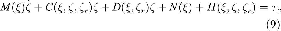
The trajectory equation of the task performed by AVVMS is given as follows

${\xi }_d\left(t\right)=\left[\begin{array}{c}1.15\times {10}^{-6}{t}^4-2.5\times {10}^{-5}{t}^3-6.4\times {10}^{-4}{t}^2+0.16t-6.2\\ -2\times {10}^{-5}{t}^5+1.6\times {10}^{-3}{t}^4-0.04t^3+0.3t^2-0.18t+0.018\\ 0\end{array}\right]\text{m}\}0\le t\le 12\text{ s}$

${\xi }_d\left(t\right)=\left[\begin{array}{c}3.7\times {10}^{-6}{t}^5+1.6\times {10}^{-4}{t}^4+0.001t^3+0.013t^2+0.18t-2\\ -4\times {10}^{-6}{t}^5+3\times {10}^{-4}{t}^4-6\times {10}^{-3}{t}^3+0.02t^2+0.4t-0.3\\ -3.3\times {10}^{-6}{t}^5+2.2\times {10}^{-4}{t}^4-0.005t^3+0.038t^2-0.1t+3\end{array}\right]\text{m}\}12<t\le 42\text{ s}$

${\xi }_d\left(t\right)=\left[\begin{array}{c}-4.7\times {10}^{-7}{t}^5+5\times {10}^{-5}{t}^4+1.7\times {10}^{-3}{t}^3+0.02t^2+0.05t\\ 2\times {10}^{-6}{t}^5-2\times {10}^{-4}{t}^4+6.8\times {10}^{-3}{t}^3-0.08t^2+0.12t\\ 0\end{array}\right]\text{m}\}42<t\le 72\text{ s}$

19

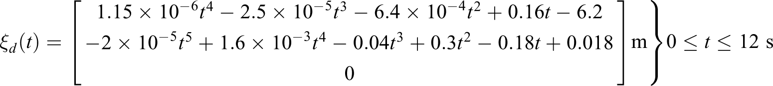
V_ed is used as the system input, and the smooth desired trajectory ξ _d(t) is constructed by cubic spline interpolation. Use the following equation to simulate the difference between expected and true kinetic parameters: $\widehat{M}=0.9 M$ , $\widehat{C}=1.2C$ , $\widehat{D}=1.2D$ , $\widehat{N}=0.75 N$ , $\widehat{\Xi }=0_{12\times 1}$ . The parameters of sliding mode controller are as follows: λ = 6, c = 16, $K_q=\text{ diag}\left\{101010101010\right\}$ , $K_d =\text{diag}\left\{101010\mathrm{15\; 20}15101010101010\right\}$ , $K_s=\text{diag}\left\{505050608060101010101010\right\}$ . The parameters of the first-order low-pass filter are $A_{\zeta d}=\text{diag}\left\{0.10.10.10.10.10.10.010.010.010.010.010.01\right\}$ . The detailed parameters of the manipulator are presented in Tables 1 and 2.

Table 1.

D–H parameters (m, rad), radius (m), and length (m) of the manipulator.

Parameters	a	d	θ	α	Radius	Length	Limits
Link 1	0.1	0	q 1	π/2	0.05	0.15	−π/2 to π/2
Link 2	0.5	0	q 2	0	0.05	0.6	−π/2 to π/2
Link 3	0.4	0	q 3	0	0.04	0.4	−2.8 to 2.8
Link 4	0.2	0	q 4	−π/2	0.03	0.2	−2.8 to 2.8
Link 5	0	0	q 5	−π/2	0.03	0.1	−4 to 0.87
Link 6	0	0.1	q 6	0	0.03	0.1	−π to π

Table 2.

Link inertia (kg m²) and viscous friction (N ms) of the manipulator.

Parameters	Ix ,i	Iy,i	Iz,i	Ix y,i	Ix z,i	Iyz,i	Viscous friction
Link 1	0.096	0.096	0.015	0	0	0	−25
Link 2	0.059	5.684	5.684	0	0	0	−40
Link 3	0.016	1.080	1.018	0	0	0	−40
Link 4	0.077	0.077	0.003	0	0	0	−35
Link 5	0.002	0.010	0.010	0	0	0	−30
Link 6	0.010	0.010	0.003	0	0	0	−30

In order to prove the superiority of the proposed control scheme, a PID controller is also used to to compare in this paper. The PID control law is as follows

$\tau =K_{p}e+K_i{\displaystyle \int edt+}{K}_d\dot{e}+G(q)$

20

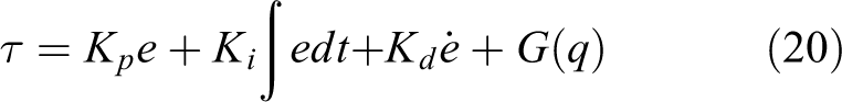
where K_p , K_I , and K_d are the proportional, integral, and derivative gain matrices of the AVVMS, respectively. This method has a quick computation and real-time performance.

Numerical simulation results

When AVVMS is in land and sky states, its paths are respectively shown by the blue and brown trajectories in Figure 5. Since the manipulator is in a nonoperating state during the land and air states, the trajectory tracking performance is uniformly described here. Figures 6 and 7 show the tracking position and orientation curve of the vehicle under the land and air states. Simulation time is 12 s and 30 s, respectively, and the simulation step size is 0.008 s. As shown in Figure 6, the proposed controller and PID controller both have good trajectory tracking effects. The position tracking error is within ±0.2 m, and the orientation tracking error is within ±4°. As shown in Figure 7, the control effect of the proposed controller is obviously better than that of the PID controller. As shown in Figure 7(a), the maximum position tracking error of the system under PID control appears near 25 s, and the error value reaches 0.1 m. Under the proposed control scheme, the error value of this time period is within ±0.05 m. Figure 7(b) shows that there is a large tracking error between the actual trajectory and the desired trajectory under PID control. And as the tracking path deteriorates, the error value increases. However, under the action of the proposed controller, the system still maintains a good trajectory tracking ability.

Figure 6.

Tracking curve of the land trajectory: (a) vehicle commanded and measured position and (b) vehicle commanded and measured heading angle.

Figure 7.

Tracking curve of the flying trajectory: (a) vehicle commanded and measured position and (b) vehicle commanded and measured orientation.

When AVVMS is in the underwater state, the position of end effector is moved from the position [0.0, 0.0, 0.0] m to the position [2.5, −0.5, −0.2] m. The trajectory is on the xy-plane and the path is shown as the red trajectory in Figure 7. The simulation time is set to 30 s and the simulation step size is 0.008 s.

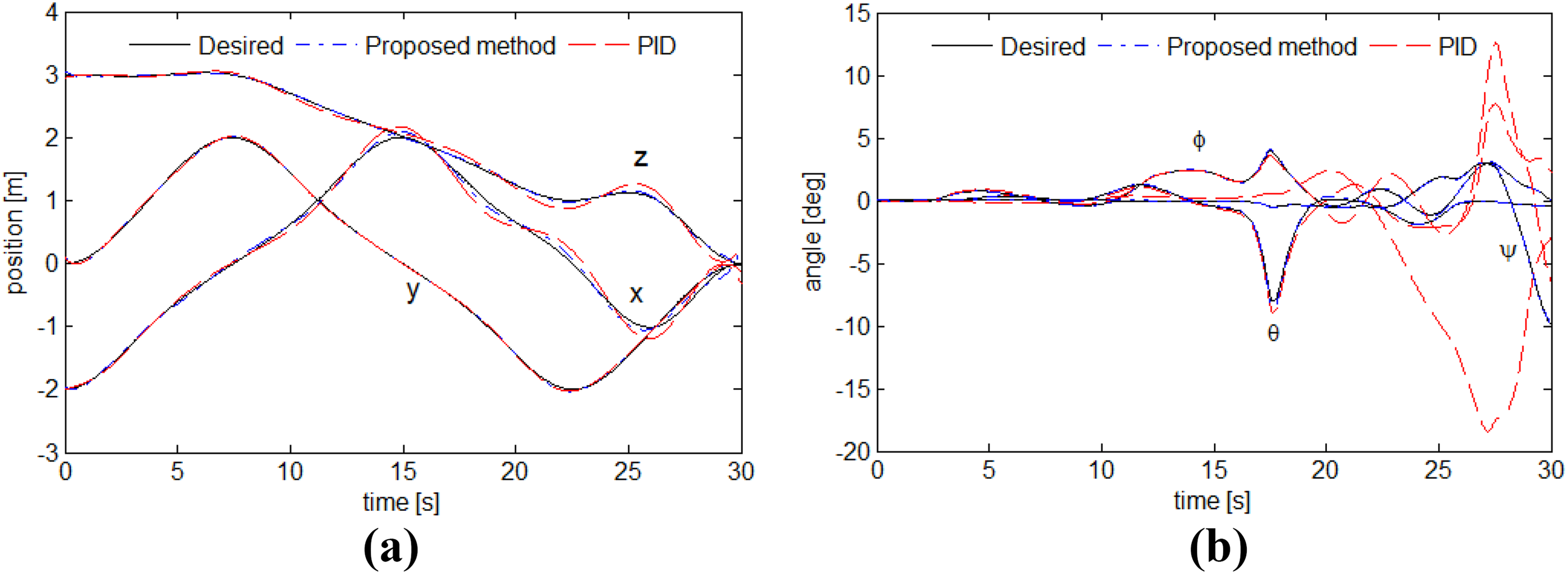
Figure 8 shows the trajectory tracking status of the vehicle. Under the control of the proposed controller, the actual position and orientation of the vehicle is almost identical to the command position and orientation. During the tracking process, the position error of the vehicle in the x-axis is significantly larger than that of the y-axis and z-axis, and the maximum error value is 0.032 m, which is caused by the largest component of the current velocity on the x-axis. Although the vehicle always has errors in the orientation tracking process, the orientation error is similar to the position error and is in a small range. It can also be seen that although the PID control method can track the desired trajectory, it has poor performance and large tracking error. Figure 9(a) shows the tracking angular state of each joint. It can be seen from the figure that under the coordinated control, the manipulator no longer remains stationary and each joint does not exceed its joint angle limit. Figure 9(b) shows that under the proposed control method, the tracking error of each joint is within ±2°. From Figure 10, we can see that under the proposed control method, the position error of the end effector is within ±0.15 m and the orientation error of the end effector is within ±3.0°, which can meet the high-precision positioning requirements of the end effector. The positional component in the z-axis is 0, this is because the command trajectory of the end effector is on the xy-plane. In addition, it can be seen from the periods of 0–5 and 13–20 s that the vehicle is in a suspension state, at which time the joints of the manipulator move within the limit of the joint angles. Since the vehicle is subjected to coupling effects and external disturbances, the controller still needs to command the power source output force/torque to maintain the pose of the vehicle.

Figure 8.

Vehicle tracking curve of the underwater trajectory: (a) vehicle commanded and measured position and (b) vehicle commanded and measured orientation.

Figure 9.

Joint angle tracking and tracking error curve of the underwater trajectory: (a) commanded and measured joint angle and (b) joint angular error using the proposed controller.

Figure 10.

End effector tracking and tracking error curve of the underwater trajectory: (a) end effector commanded and measured position and (b) end effector commanded and measured orientation.

Figure 11 shows the control force/torque of AVVMS under the effect of the proposed control method. Figure 11(a) shows the control force/torque of the vehicle. It can be seen from Figure 11(a) that the force fluctuations acting on the substrate at 0–5 and 13–20 s are small, and are mainly used to maintain the stability of the vehicle. At the same time, it also can be seen that when the vehicle is switched between the action and the stationary suspension state, the force/torque appears to be dithered at this moment. Fig. 11(b) shows the manipulator control torques. It can be seen that the controller assigns a larger torque to joints 1, joints 2 and joints 3, while assigns a smaller control torque to joints 4, joints 5 and joints 6. This is consistent with the actual physical structure of the manipulator, and it also reflects the established system dynamics model and the design of the sliding mode control law are reasonable. According to the control force/torque curve, on one hand, the corresponding relationship between the driving force outputs by the sliding mode controller and the system motion can be visually observed, and on the other hand, the selection basis of the motor and propeller can be provided.

Figure 11.

Control force/torque curve of the system under underwater trajectory: (a) control force and torque to vehicle and (b) control torque to manipulator.

From the above analysis, the established kinematics and dynamic models are correct, and the quadratic computational optimization algorithm for inverse kinematics solution and the sliding mode control law are effective.

Conclusions

With “bevel variant” power switching mechanism and multi-degree of freedom manipulator, the robot’s working ability can be greatly improved. The control system built by the quadratic computational optimization algorithm for inverse kinematics solution and the sliding mode control law shows that AVVMS has a good trajectory tracking ability even under the uncertainty of kinetic parameters and external interference. The end effector can achieve higher positioning accuracy. When the system is in the land and the flying stages (the manipulator is fixed), the vehicle position and posture tracking error are within ±0.05 m and ±2.0°, respectively. When the system is in the underwater stage (the robot and manipulator are in a coordination state), the end effector position and orientation tracking error are within ±0.15 m and ±3.0°, respectively. However, the issue of how to properly control the rotation angle of the “bevel variant” power switching mechanism to enable the AVVMS to utilize energy efficiently has not been further studied. In the future, we will solve this problem to ensure that the mechanism can be applied to the actual.

Supplemental material

Supplemental Material, Appendix_A - Trajectory tracking control of an amphibian robot with operational capability

Supplemental Material, Appendix_A for Trajectory tracking control of an amphibian robot with operational capability by Fujie Yu and Yuan Chen in International Journal of Advanced Robotic Systems