
Abstract
The traditional homogeneous transform maintains central position in the kinematic modelling of robotics. However, for these kinematic modelling of wheeled mobile robots over uneven terrain, the homogeneous transform that represents angular velocity implicitly in the time derivative of the rotation matrix has a drawback in orientation representation. In this article, to improve the angular representation, a new general systematic method for kinematics modelling and analysis of wheeled mobile robot is proposed. The approach uses the Sheth–Uicker convention and loop-closure kinematic chains to derive the position, velocity and acceleration kinematics. The screw coordinates are used to reform the velocity kinematics to centroidal kinematics; then, the Jacobian calculation is simplified to solve the screw vector algebra equations instead of the matrix equations. Meanwhile, the linear and angular components of the centroidal kinematics are endowed with physical meanings and are easy to be selected as control variables. The approach is applied to a wheeled mobile robot, and its effectiveness is verified by the simulation results with various terrain.
Introduction
As the same to the serial manipulator, kinematic models play an important role in forward and inverse kinematic analysis in wheeled mobile robots (WMRs). In complicate task, the kinematic models are used to map desired motions of WMR to actuators’ motion and estimate motion states of WMR by sensed degrees of freedom (DOFs) in the same time. 1 For more details, the kinematic model has been applied to navigation kinematics, slip kinematics and actuation kinematics. 2
There are new challenges for kinematic models when WMRs are in the condition of obstacle overcoming (inclined terrain, step climbing, trench crossing etc.). Posture information with oriented description should be emphasized in the kinematic model. Active adjustment of postures requires information from a given trajectory converted to the actuated joints; moreover, state estimation of WMRs’ posture with respect to the terrain requires perception information that converted from the actuated joints.
During the research efforts on kinematic analysis of different WMRs, methodologies were summarized to adapt to different engineering applications. Although many researchers have introduced these methods in some aspects, it is indeed worthwhile to classify and compare these methods to make further technological progress.
Homogeneous transform method
This method is characterised by the homogeneous transformation matrix in the robotics to derive kinematics. Muir and Neuman 3,4 used Sheth–Uicker convention and instantaneously coincident coordinate systems (ICCS) to formulate systematic kinematic equation. The ICCS was used to calculate velocities of robot body and wheel contact points. However, time differentiation operation must follow their own algebra axioms rather than a mathematical differential operation, which limited its more general applications. Rajagopalan 5 extended the approach to WMRs with steering axes that were not orthogonal to ground. Dong and Park 6 modified the planar pair assumption of wheel motion to a point-contact high pair. Tarokh and McDermott 2 extended the motion of wheel to uneven terrain by wheel contact angle and associated the velocity of robot body derived by ICCS with the differential motion of WMR. On the basis of Tarokh and McDermott’s work, Chang et al. 7 rearranged the kinematic equation. The angular velocities (represented by product of a skew-symmetric matrix and an orientation rate vector) and linear velocities of robot body were separated in the systematic kinematic equation. The Jacobian matrices mapped the separated motions of robot body in translational and postural to the physical conception about parameters defined by configuration of robot.
Vector algebra method
The physical basis of this method is the Transport Theorem of composite motions. The relative motions between articulated linkages were expressed as composite motions of a fixed frame and a moving frame in vector form. Grand et al. 8,9 formulated the velocity equation of each wheel contacted with the ground in closed form; then, full system kinematic model composed of all wheel-leg chains equation expressed by projecting to the local wheel contact frame was formulated. Chang et al. 10 employed this approach to formulate the vector expression of the wheel centre velocity in the robot body frame and contact point frame, respectively; then, the kinematic equation of each wheel centre’s velocity was projected to the robot frame to formulate the systemic kinematic equation. This way of modelling was summarized as wheel centre modelling method. Kelly 11,12 explained the vector algebra method based on Transport Theorem in detail in his report and monograph and extended the wheel contact model with non-holonomic constraints in the kinematic equation. Later, Kelly and Seegmiller 1,13 further developed this method as recursive kinematic propagation approach. Once the known quantities of linear and angular velocities in the equations were formulated, they would propagate in the kinematic chain and unknown quantities could be solved recursively.
Screw-based method
There are two advantages to kinematic modelling of WMRs using screw theory. The first is that it can describe rigid body motion in global frame which avoids singularities due to the use of local frames. The second is that screw theory simplifies the analysis of mechanisms by geometric description of rigid motion. 14 The kinematics model of WMR could be modelled as moving parallel mechanisms. 15 Le Menn et al. 16 proposed a generic differential kinematic modelling method and pointed out that the velocity equations of input/output were an extension of reciprocal screw method applied on parallel mechanisms. Without using joint screws, Fu and Krovi 17 extracted the twist vector from twist matrix of homogeneous transform matrix and established the kinematic screw equation by the twist vector and its adjoint transform matrix. Yi et al. 18 derived the inverse kinematics of independent joints with respect to the system twist by inner product of each reciprocal screw and system output twist. In obstacle clearing analysis, by systematic screw kinematic model, Benamar et al. 19 obtained force–moment transmission matrix of central body in wrench space which was equivalent to grasp matrix in grasp mechanism and proposed the concept of global traction ellipsoid derived from force-moment transmission matrix to evaluate the obstacle clearance capability.
It is necessary to summarize the commonalities and differences of these three kinematic modelling methods to clarify the direction of improvement. Firstly, the WMR is assumed as moving parallel multichain mechanisms in these methods; the vector algebra method and screw-based method treat WMR as multiple open chain structures; the homogeneous transform method adopt the loop-closure chain structure because its convenience in derivation of position kinematics and velocity kinematics; however, no matter the algebra axioms in the study by Muir and Neuman 4 or later improvements by Tarokh and Chang, the matrix operations are not uniform and need to be improved to make consistent with operations in robotics. Secondly, the wheel contact angle is accepted to describe wheel contact on uneven terrain; however, the wheel slip assumption is at variance. Representatively, Tarokh and colleagues 2,20 derived slip kinematics to predict various wheel slips; however, Muir and Neuman 4 and Kelly and Seegmiller 1 assumed that wheel slip was known or supposed to be negligible for the view that wheel slip was a problem that out the scape of kinematic analysis and it could be easily measured in vehicle level. In this article, the wheel slip was neglected to focus on kinematic analysis. Thirdly, the modelling of oriented motion is in demand apparently; it is represented by angular velocity in vector algebra method and by twist motion in screw-based method. The oriented motion relationship between central body and independent joint in these two methods can be expressed straightforward; however, orientation modelling in homogeneous transform method needs to be improved to achieve the requirement.
According to the comparison of these three kinds of kinematic modelling methods, we can find that in the kinematic modelling of WMRs, the homogeneous transform method is competent in handling the parallel multichain and contact angle; however, it has shortcoming in terms of modelling the oriented motions of WMRs. The goal of this article is to propose a systematic approach for kinematic modelling for WMRs to deal with the complexity of the WMR mechanism, multiple parallel closed chain kinematics and description of the linear and angular motion over uneven terrain.
Tarokh and McDermott 2 extended Muir’s modelling method to uneven terrain; however, their work only focus on velocity kinematics. The recursive velocity kinematic modelling method 20 was used to deal with the connection of rover mechanism recursively, but the Denavit–Hartenberg table (DHT) based on Denavit–Hartenberg convention lost generality and intuitiveness in describing the complexity of spatial motion of WMR. Chang et al. 7 mixed the separated linear and angular components of velocity together to represent the wheel centre velocity; however, the combined velocity was hard to separate in the actual control target design. Compared to previous works 2,7,20 , we derive our approach starting from the Sheth–Uicker convention and closed-loop chains. The convention let us facilitate the modelling of the complicated WMR mechanism and uneven terrain topology, and we derived position, velocity and acceleration kinematics based on the loop-closure equation. Moreover, we explicitly state the angular velocity by convert velocity kinematics equations to screw coordinates equations rather than encoded as the time derivative of a rotation matrix.
We believe that the main practical significance of our work is the centroidal kinematics consisting of velocity kinematics improving the inadequacy of homogeneous transform method in terms of the orientation expression[AQ; Please approve edit made to the sentence ‘We believe that the main practical…’.]. The centroidal kinematics decouple the DOF of WMR’s central body to the DOF of actuated joints to meet the challenge of active control of posture adjustment to adopt to the uneven terrain. The centroid velocity, with all or part of the linear and explicit angular components are selected, facilitates the design of the control target (see ‘Screw property of velocity kinematics’ section).
This article is organized as follows. In the second section, the proposed improved homogeneous transform method by Sheth–Uicker convention is described in detail, and the screw property of velocity kinematic is explained. In the third section, the application of the approach to a WMR with 18 DOFs is described. In the fourth section, simulations of the WMR traversing several terrain topologies are performed in order to verify the motions of articulated linkages with desired central body posture. Finally, the fifth section gives the conclusions of this article.
Contributions
We proposed a systematic kinematic modelling method based on Sheth–Uicker convention and closed-loop kinematic chains for WMR. The amended homogeneous transform method fits the requirement of linear and angular kinematic descriptions of WMR over uneven terrain.
On top of the main contribution, this article presents several other contributions: We present a three-dimensional (3D) prismatic joint to deal with the complicated wheel-terrain contact over uneven terrain (see ‘Coordinate arrangement and joint characteristics modelling’ section). We discuss the screw property of the velocity kinematic to reform it to be a centroidal kinematics (see ‘Screw property of velocity kinematics’ section).
Kinematic model development and analysis
WMR that with high mobility moving on uneven terrain consists of a central body, articulated linkages, wheels and joints. Posture of central body can be actively adjusted to comply with uneven terrain. In this section, we will introduce the kinematic modelling approach and formulate the position kinematics, velocity kinematics and acceleration kinematics of WMR.
The assumptions about the motions of a WMR are made before kinematic modelling: Connections between the articulated joints have no friction and damping efforts. The wheels of WMR roll on the floor without any translational slip. Skid-steering of WMR only implements displacement in the y-axis without lateral slip.
Based on the structural analysis, the WMR is modelled as multiple closed-loop chains from central body to shoulder joints, wheels and the wheel contact points. Connections between two bodies in the kinematic chain are modelled as kinematic pairs. Relative motions of joints are described by Sheth–Uicker convention after recognizing the types of kinematic pairs.
Although Sheth–Uicker convention is used in homogeneous transform method, its effort is far more underestimated. Sheth–Uicker convention is sometimes considered as a complicated convention that is only useful for parallel mechanism modelling; however, compared to the Denavit–Hartenberg convention, the convention extends the two-axial twist description of mechanism to three-axial twist. Thus, the Sheth–Uicker convention generally features the right degree of complexity of arbitrary mechanisms and is suited to describe a mechanism in the form of tables according to the topologies of the mechanism type. 21 We will introduce our new method completely based on Sheth–Uicker convention and give the results that are consistent with screw theory. Detailed descriptions of Sheth–Uicker convention are available in the literature. 21 –23
Coordinate arrangement and joint characteristics modelling
The assumptions of kinematic pairs are described as follows: the relative motion between the central body and the floor or ground is assumed to be an open joint (referred as open joint); the rotations between the articulated linkages and the central body are assumed to be revolute joints (referred as shoulder joints); the relative motions between the wheels and the floor are assumed to be revolute joints (rotation between the articulated linkage and the wheel) and 3D prismatic joints (Figure 1; referred as LW joint and wheel joint, respectively). Coordinates arrangement is related to kinematic pair assumption; each joint has four coordinates with two fixed coordinates on the two moving bodies and two moving coordinates related to the joint. In our arrangement, the world frame is coincident with floor frame. The floor frames in the open joint and wheel joints are merged into one frame. The results of frames arrangement are shown in Figure 2.

Wheel–terrain contact modelled as revolute joint and 3D prismatic joint. 3D: three-dimensional.

Coordinate frames of WMR. WMR: wheeled mobile robot.
We will describe the assumption of each joint in detail and give the transformation matrix between two bodies according the assumed joint.
The open joint has six DOFs motions with three DOFs prismatic movements and three DOFs revolute movements in Cartesian coordinate system. Its joint variable is defined as

The origin of floor frame

where SFO is the shape matrix from floor to open joint ΦO and SRO is the shape matrix from robot central body’s COM to open joint ΦO , both SFO and SRO are unit matrices.
For the shoulder joint, it has only one variable, qi , and the joint transformation matrix can be written as

Similarly, transformation matrix from central body to the articulated linkage is

where
As shown in Figure 1, the wheel–terrain interaction assumption, related to wheel–terrain contact, is separated to revolute LW joint and 3D prismatic wheel joint, which because of that the angle between the linkage and the wheel cannot be integrated into the rotation submatrix of 3D prismatic wheel joint. In the LW joint, the angle between the linkage and the wheel is caused by the interaction of posture of the WMR and the profile of terrain. The joint is defined to be
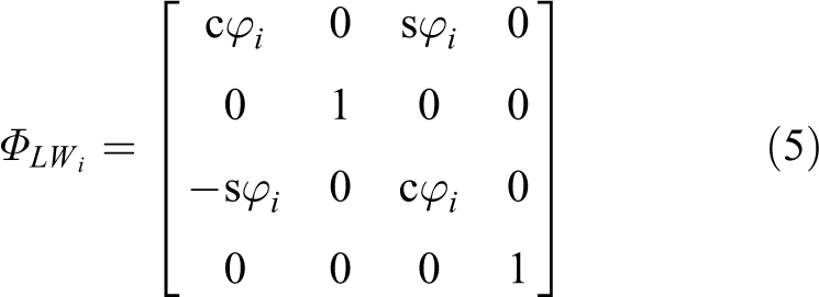
where the angle φi represents the angle between wheel and articulated linkage, and it is also related to the wheel contact angle σi . The relation can be formulated by geometrical dimension between central body’s COM and wheel’s rotating centre in inverse kinematics.
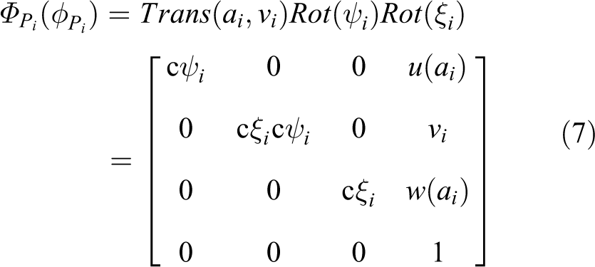
The transformation matrix from articulated linkage to wheel is

The 3D prismatic wheel joint is revised from the point on a planar-curve joint with its original definition in 23. In order to fit the wheel–terrain contact assumption, modifications to the joint are necessary. The
Additional descriptions to the angles ψi
and ξi
are that they are caused by central body’s yaw and roll motion, respectively. Terrain topology information is implicated in the functions
Finally, the transformation matrix from the ith wheel to origin of floor frame is

Closed-loop mechanism modelling
With the connections of the open joint, shoulder joints, LW joints and wheel joints, multiple closed-loop chains are formed by the paths from the origin of floor frame, robot central body, articulated linkages, wheels and back to the origin point. Methods dealing with closed-loop chain need to be chosen restrainedly as they are the basics of the position kinematics, velocity kinematics and acceleration kinematics. The equivalent tree-structured method 24,25 virtually cuts the closed chain at a non-actuated joint to obtain an equivalent tree-structured open chain and computes kinematics function by composing various transformations from base frame to end-effector frame. However, it is difficult to deal with the selection of non-actuated joints in all-actuated structure of WMRs. With closed-form transformation graph and ‘matrix transformation algebra axioms’, 4 Muir’s transformation matrix method can easily treat with the closed-loop chain problem in position kinematics, but differential operation is also restricted to their algebra axioms. According to fundamental conclusion of the closed-loop chain, it always returns back to the original coordinate frame when consecutive transformations are made, no matter which body is chosen as a starting body. The matrix product must equal the identity transformation – the (4 × 4) unit matrix. 23 With the fundamental conclusion, kinematic matrix equation for position analysis can be formulated in global coordinates.
The kinematic loop-closure matrix equation of the closed-loop chain is as follows

Position kinematics
In the practical control, the absolute positions of each body of WMR with respect to the floor frame are needed for localization and navigation. They can be easily derived without further transformation due to our coordinate assignment. Besides absolute positions, relative positions may be calculated by known transformations. Position transformation graph (Figure 3) can be used to determine cascaded transformation matrices to derive desired transformation of absolute or relative position. Either in direct or in inverse direction, the usage of transformation matrix or its inverse matrix depends on the direction of arrow. For example, the transformation matrix from robot central body to articulated linkages can be derived by

Transformation graph of a WMR. WMR: wheeled mobile robot.
By equation (9) and the transformation graph, we derive the following kinematic results:
Forward position kinematics:
Inverse position kinematics:
We must emphasize that transformation graph can be used in any complicated closed-loop chain even though the demonstrated closed-loop is simple.
Velocity kinematics
In the velocity kinematics, there are two items to deal with. One is the absolute velocity of a body of WMR, and the other is the systematic velocity kinematic equation. Before differentiating the closed-loop matrix equation (9) to derive velocity kinematic equation, we should analyse the differential motions of the joints of WMR. A general differential motion that contains differential translations and differential rotations can be written as 26,27
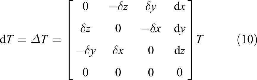
where Δ is the differential operator matrix of a general transformation matrix. We calculate the derivative of joint Φh with respect to its joint variables ϕh to be

where Qh denotes the derivative operator matrix of joint Φh .
The derivative operator matrix of the open joint ΦO can be derived as

Meanwhile, the derivative operator matrices of the shoulder joint,


and

Next, we will calculate the absolute velocity of each body in the closed-loop chain. In a general form, we define the absolute velocity of body b caused by joint Φh
, and the transformation matrix of body b in floor frame is

During the simplification, insertion of appropriate identity factors is necessary and
Let us define another derivative operator matrix

The absolute velocity of robot central body is

The absolute velocity of an articulated linkage is

The absolute velocity of a wheel is

Note that according to the definition of Qh
, the

Velocity kinematic equation is derived by time derivative of the closed-loop equation (9). The expression is as follows
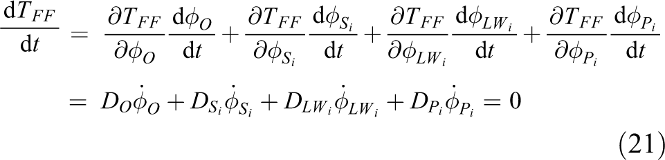
Equation (21) is the fundamental result of velocity kinematics; the motion of the central body is naturally separated from motions of these joints. It is also used to construct forward and inverse kinematics.
Forward kinematics
Forward kinematics or sensed kinematics calculates velocity (linear and angular) of the central body from the sensed velocities of shoulder joints and wheel joints. Equation (21) is rewritten as follows by moving sensed quantities to the right

It is clear that the velocity relationship between velocity of central body and other joints in the closed-loop chain will be a Jacobian matrix. The derivative operator matrix of open joint is an identity matrix due to the coordinate assignment, so it is convenient to derive Jacobians from forward kinematics. Variables in velocity
Inverse kinematics
Inverse kinematics is to decompose the trajectory information (position, orientation, linear velocity, angular velocity etc.) of the central body into the motions of the shoulder joints and wheel joints. Inverse kinematics is mainly related to control topics; main parameters of the control target can be defined according to WMRs’ different working conditions (steering, side slope, step climbing etc.). Equation (21) is rearranged to show the relationship of wheel joints with other joints

The shoulder joint is handled in the same way

Even though it is complicate, equations (23) and (24) can also be used to derive Jacobians.
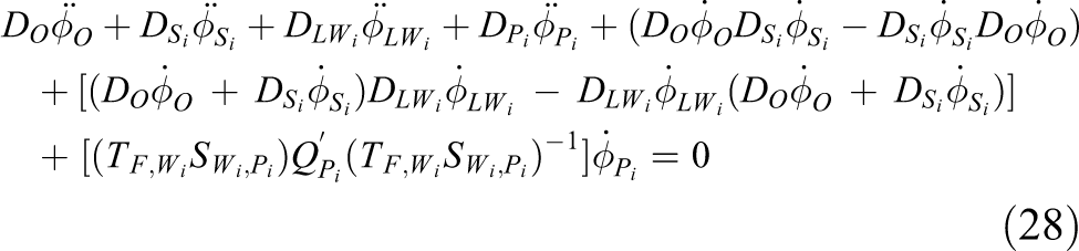
Acceleration kinematics
Acceleration kinematics that is used to compute forces and moments in dynamic analysis is needed in real applications; however, differentiation of both sides of a transformation matrix equation to formulate the acceleration equation is not an allowable operation; 4 moreover, formulation of acceleration is not mentioned. 2 We want to emphasize that our formulation of the acceleration equation which based on the time derivative of kinematic velocity equations is complied with mathematical derivative operations. Systematic acceleration equation is derived from time derivative of equation (21)

According to the definition in equation (16), time derivative of derivative operator matrix Dh is calculated as follows

Time derivative of derivative operator matrix Qh needs to be calculated during the simplification of the time derivative of Dh . It can be written as

where
Substituting the absolute velocity of body (equations (17) to (19)) in the closed-loop chain into equation (26), and equation (25) is reduced to by equations (26) and (27)
The last item of matrix product is not written in simple form, because parameters in matrix
Screw property of velocity kinematics
Featherstone
28
defined a six-dimensional (6D) spatial vector to represent the combined linear and angular components of the physical quantities involved in rigid-body transformation. A (6 × 6) spatial transformation matrix, similar to (4 × 4) homogeneous transform, is defined to describe a general spatial coordinate transform (named Plücker transform). The (6 × 6) spatial transformation matrix is the adjoint matrix of a general homogeneous transformation matrix
14
; moreover, the six independent elements of derivative operator matrix Qh
can be represented as a 6D vector

The derivative operator matrix Dh
, in the general form of
The equivalent


and

Finally, the matrix equations (22) to (24) are replaced as six algebraic equations, respectively. The six algebraic equations express the rates of changes (with three translational changes and three rotational changes) in their own coordinate direction, respectively. This operation not only reduces the number of equations, but also benefits the selection and definition of target goals in the actual control. In actual application, related to control topics, one or more physical components are combined to accomplish a specific function, such as steering, pitch angle adjustment, side slope driving and so on.
Reference WMR
In this section, we will apply the general result of the last section to a concrete case in symbolic form. We will illustrate the application of kinematics to our 18 DOFs platform named unmanned grounded vehicle with articulated suspension (UGVAS). The UGVAS is designed to be a central body with six articulated linkages, and each linkage is articulated with a wheel. As assumed in ‘Coordinate arrangement and joint characteristics modelling’ section, the shoulder joints and wheel joints are all actuated. As shown in Figure 4, the distance between two shoulder joints is l1, the distance between COM of central body and shoulder joint is h, the length of linkage is l2, the radius of wheel is r, the width of the two shoulder joints is 2b, d denotes the distance of wheel joint to shoulder joint in vertical projection direction and
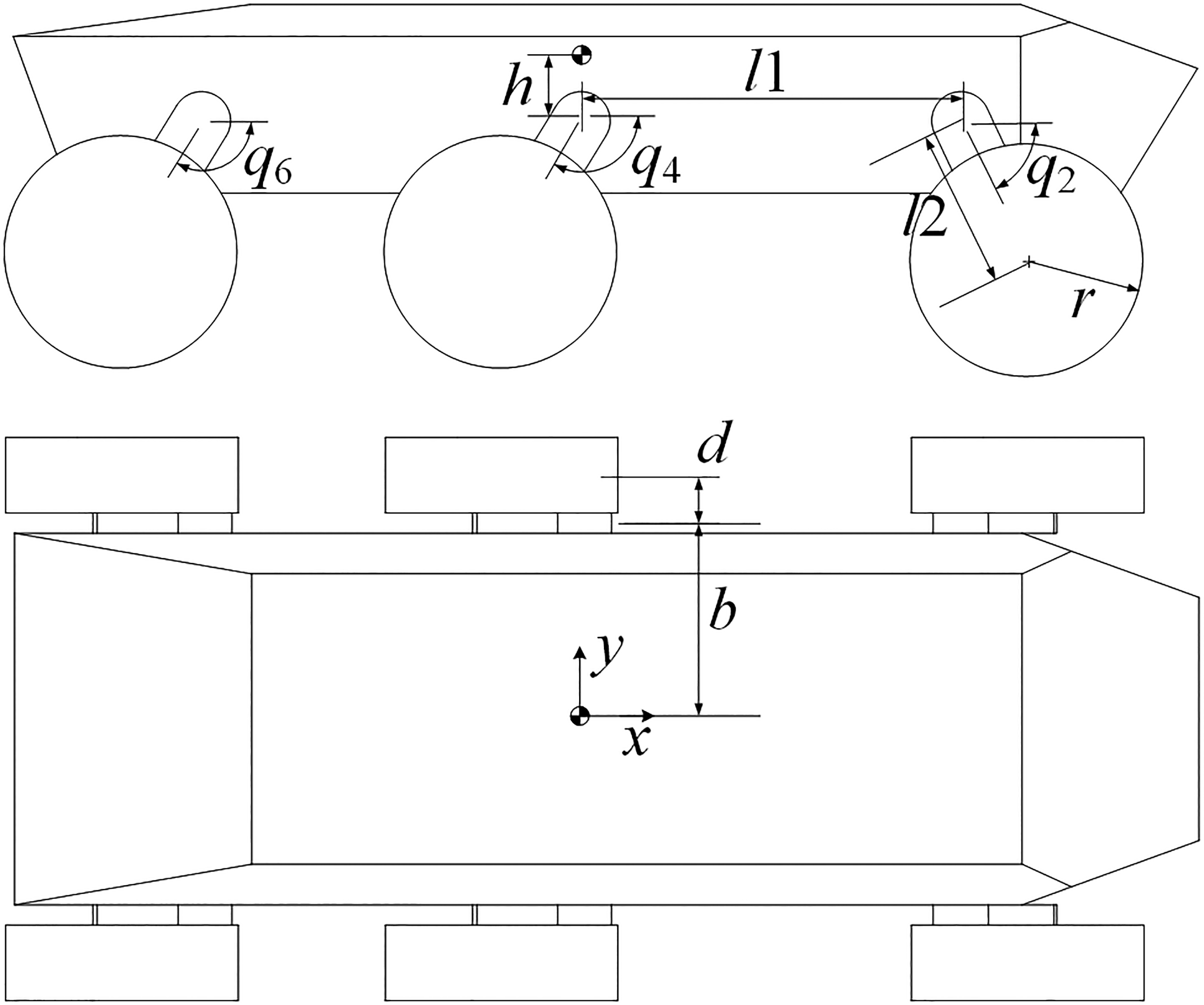
UGVAS design. The articulated linkages can be actively actuated to accomplish required posture with respect to uneven terrain. UGVAS: unmanned grounded vehicle with articulated suspension.
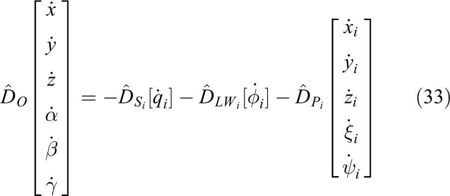
Let us reiterate the two topics related to the application of kinematic equations, state estimation and control. Forward kinematics: calculating the motion of central body from measured motions of shoulder joints and wheel joints. Inverse kinematics: translating the desired motion of central body to the equivalent motions of shoulder joints and wheel joints.
For the purpose of a general application, six components of the open joint ϕO are all participated in the derivation of Jacobians. Calculating the Jacobians by forward kinematics, equation (30) is expanded as
We produce the results by symbolic math software and give
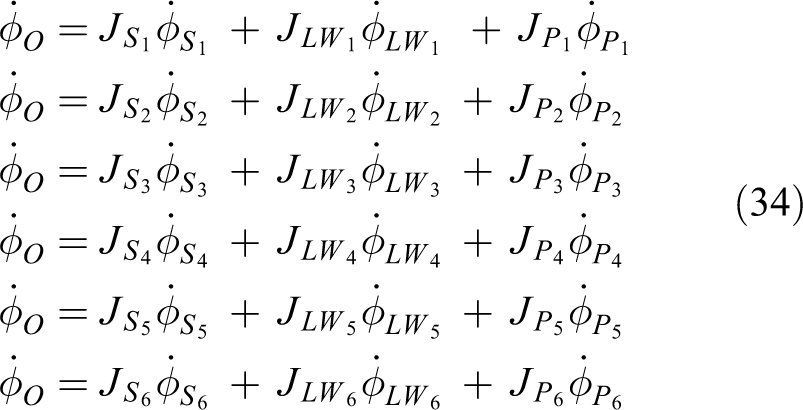
where
Stacking all equations in equation (34) together, we get

where
Matrices J S, J LW and J P are the three Jacobians involved in forward kinematics, and they are related to the shoulder joints, LW joints and wheel joints, respectively.
The inverse solution of the shoulder joints can be derived from equation (35) by moving all known quantities to the right

This can be solved by the pseudoinverse method

The inverse solution of the wheel joints can be derived in the same way

Simulations
In this section, we discuss the application of kinematics to the posture control of our platform UGVAS in several scenarios. The works are accomplished by simulations in the Simscape Multibody. The simulation model consists of several modules as shown in Figure 5. The trajectory module gives the desired position velocities and posture turning rates of UGVAS as a function of time. The inverse kinematics module produces actuation signals to the actuate joints of UGVAS, and this module uses the desired trajectory and the current states information such as robot central body’s roll, pitch and yaw angles, revolute angles of shoulder joints and LW joints, terrain and platform interaction information and so on. The forward kinematics module is used to calculate the current states from sensors.

UGVAS control block diagram. UGVAS: unmanned grounded vehicle with articulated suspension.
Terrain topology is generated by a mathematical function
In the simulation, the dynamic behaviour is not considered since the relatively slow motion is set in the trajectory. Wheel slips that occur in uneven terrain are neglected as mentioned before; however, investigations about them are undergoing. It must be emphasized that the following cases focus on the verification of kinematic modelling.
The platform is set to be travelled on several uneven surfaces and controlled uniquely oriented and located in the global coordinate system. Some of the simulation scenarios are inspired from. 20 In the simulation, relative to the linear velocities, we put particular emphasis on the variations of angles of articulated linkages with respect to the angular changes of central body.
Case 1: Inclined surface
The terrain is a slope of 20° inclined smooth surface as shown in Figure 6(a). The platform moves upward the slope along a straight line with 9500 mm distance of travel in the x-axis. The pitch angle of the platform is reduced from the initial angle of 20° to 10° as shown in Figure 7(a) to make the platform lean forward to keep the central body of the platform relatively flat. The angles of articulated linkages are shown in Figure 7(b), and it is seen that the angles of front linkages q
1 and q
2 decrease from

(a) UGVAS moving upward a 20° slope and (b) UGVAS moving on an inclined circular path. UGVAS: unmanned grounded vehicle with articulated suspension.
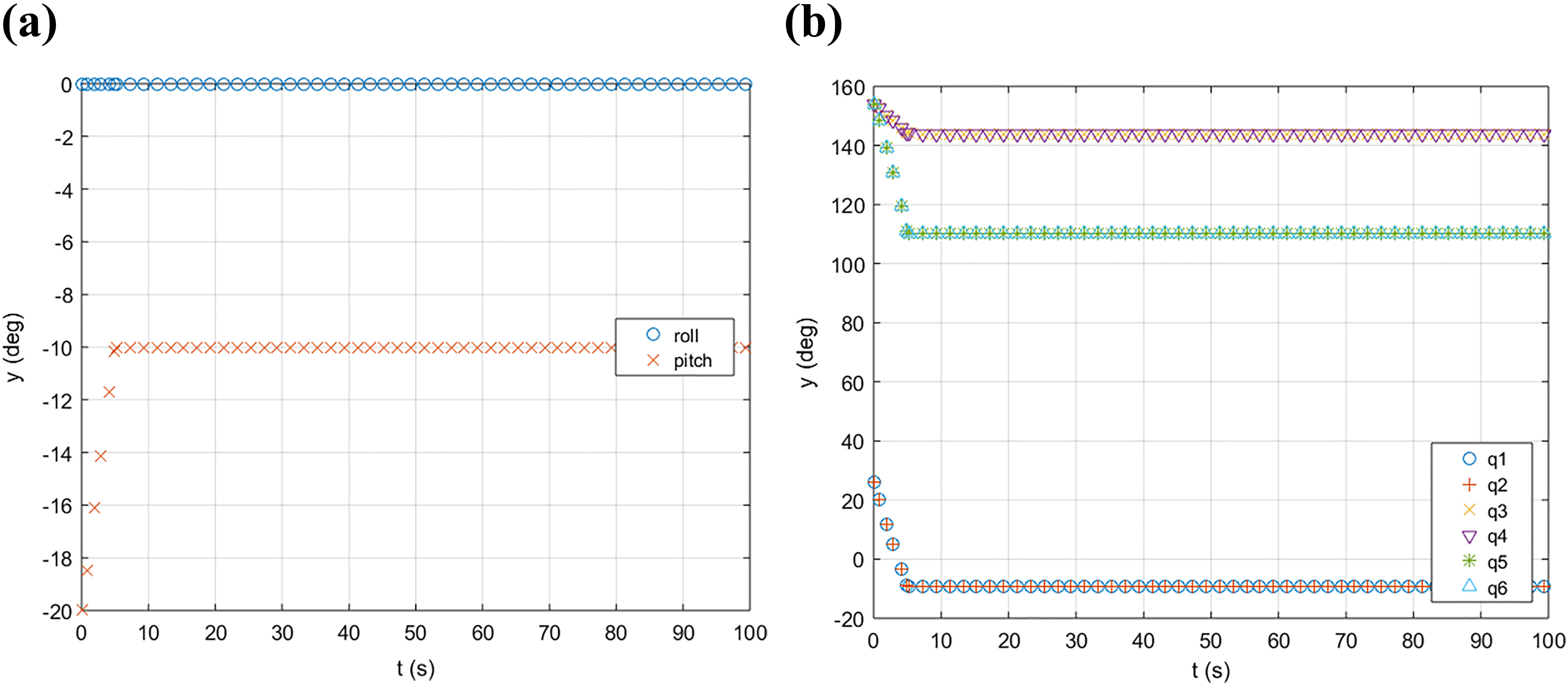
(a) UGVAS central body roll and pitch for the inclined surface and (b) articulated linkage angles. UGVAS: unmanned grounded vehicle with articulated suspension.
Case 2: Circular path on inclined surface
In this case, the platform is considered to travel on a 20° slope of inclined surface and is constrained in a circular path as shown in Figure 6(b). The time trajectories of Cartesian coordinate are given by

(a) UGVAS central body roll and pitch for the circular path and (b) angle variations of the articulated linkages. UGVAS: unmanned grounded vehicle with articulated suspension.
Case 3: Bumpy terrain
In this case, as shown in Figure 9(a), we consider an asymmetrical bumpy terrain with one side of terrain with unequal spacing and radius circular bumps and the other side of a flat terrain. The elevation of the bumpy terrain is given by
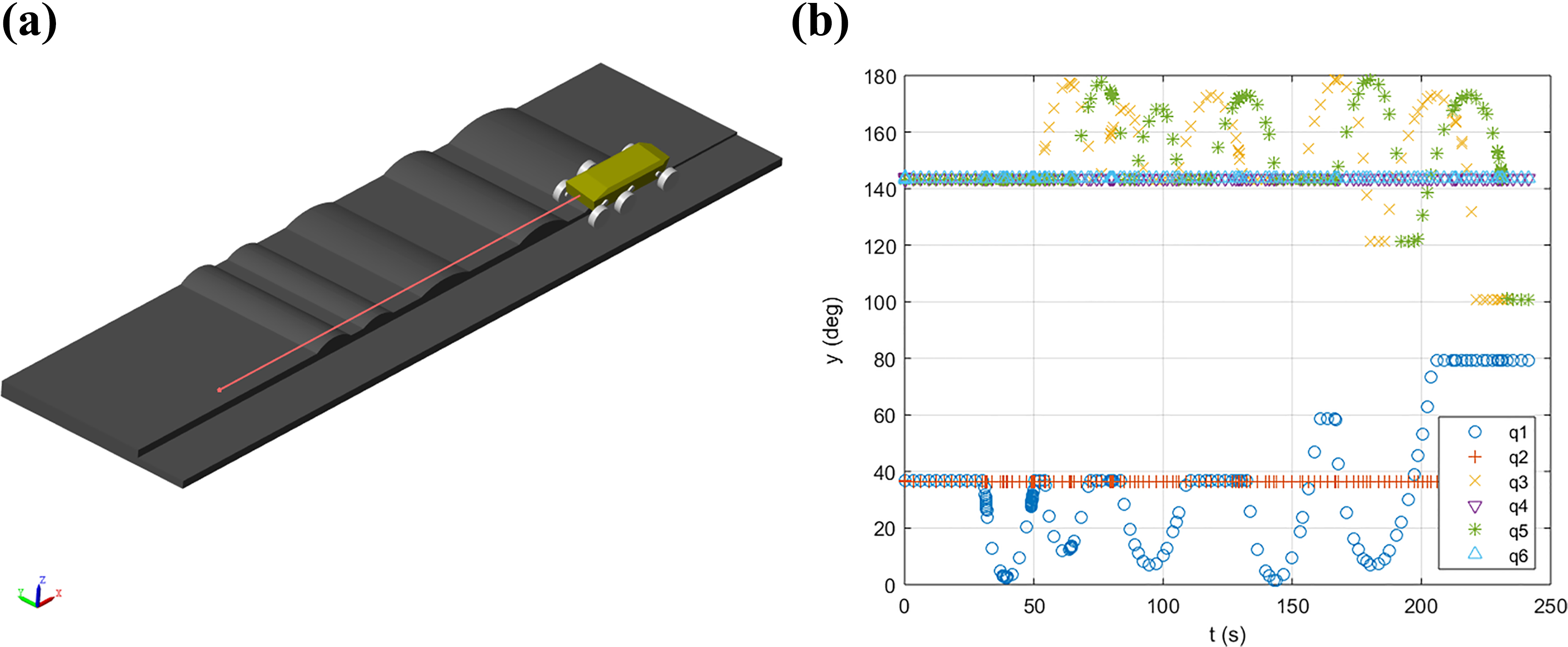
(a) Asymmetrical bump terrain and (b) angle variations of the articulated linkages.
Conclusion
The differentiation of the homogeneous transform has limited our understanding of WMR kinematics; the result represents angular velocity implicitly. In this article, we summarized and compared three kinds of kinematic modelling method applied in WMRs, and a new kinematic modelling methodology based on homogeneous transform method for WMRs is introduced. The approach uses the Sheth–Uicker convention and closed-loop kinematic chains to modelling the complexity of mechanisms and terrain topology. With the closed-form solutions, the position, velocity and acceleration kinematics are derived. We use screw coordinate to rewrite the velocity kinematics, and let the linear and angular velocity represented explicitly. The velocity kinematics with apparent physical meanings is convenient to be converted to the target variables in control and state estimation.
The proposed method is general and can be applied to the kinematic analysis of any WMR. It can be performed by symbolic or numeric operation and is suitable for computer implementation. The defined joint derivative operator matrix and the joint homogeneous transform matrix can be listed and stored according to the type of the joint and can be programmed as common function which will make the computer implementation very efficient.
The developed kinematic model based on this method is applied to a WMR with 18 DOFs. The simulation results of adjustments of the WMR both in position and in orientation demonstrate that the approach has the potential to handle the complicated control requirement on uneven terrain.
Footnotes
Declaration of conflicting interests
The author(s) declared no potential conflicts of interest with respect to the research, authorship, and/or publication of this article.
Funding
The author(s) received no financial support for the research, authorship, and/or publication of this article.
Appendix 1
The following matrices are the submatrices of Jacobians calculations needed in equation (34) of the third section