
Abstract
This article aims to improve the accuracy of each joint in a manipulator and to ensure the high-speed and real-time requirements. A method called the variational method genetic algorithm radial basis function, which is based on a combination feedback controller, is proposed to solve the optimal control problem. It is proposed a combined feedback with a linear part and a nonlinear part. We reconstruct the manipulator’s kinematics and dynamics models with a feedback control. In this model, the optimal trajectory, which was solved by the variation method, is regarded as the desired output. The other one is also established an improved genetic algorithm radial basis function neural network model. The optimal trajectory is rapidly solved by using the desired output and the improved genetic algorithm radial basis function neural network. This method can greatly improve the speed of the calculation and guarantee real-time performance while simultaneously ensuring accuracy.
Introduction
Mechanization, automation, and intelligence are ultimate goals in the development of industrial production. Industrial processes usually involve various manipulators. 1 The linkage manipulator is one of the most common types of manipulator and has been widely used in vehicle assembly, industrial production, food processing, and other production activities. In addition, the linkage manipulator can be used in harsh environments that are unsuitable for manual operation, such as unknown environment exploration, aerial work, and risk investigation. As optimal control problems, this process not only requires higher accuracy and speed but also is expected to require less energy, shorter time, and better robustness.
The optimal control problem of the link mechanism has already exceeded the requirements of mechanization and automation. In traditional research, direct or indirect methods can be used to solve the optimal trajectory. These methods cannot meet the needs of practical application in terms of accuracy and speed. Therefore, the research of optimal control must be made more intelligent. Various research focuses on how to combine the optimal control problem and the artificial intelligence algorithm to improve the performance of the manipulators, which has become a hot issue both at home and abroad. Three main categories of related research exist. The first type is the combination of optimal control and artificial neural networks (ANNs). For example, Boukens et al. use ANNs to control the optimal trajectory. 2 Hu et al. use multilayer perceptron (MLP) to calculate the optimal trajectory of the manipulator. 3 Moldovan et al. use the feed-forward ANN as a nonlinear autoregressive model with external inputs. Their study selects the best parameter representation of ANN to make it as close as possible to the 6-PGK prototype robot dynamics model. 4 This type of research is characterized by one advantage and two disadvantages. The advantage is that the trained neural network can solve the optimal state quickly, greatly improving the efficiency. The first disadvantage is that the weights in the ANN are not well adjusted with valid sample data for the manipulators. In an ANN, the accuracy of the results obtained by adjusting the weights according to valid sample data is better than when random weights are used. The second disadvantage is that the expected output in the training sample does not emphasize how it is obtained. The expected output is not guaranteed to be the optimal solution. Theoretically, in practice, the output could not be an analytic solution but an approximate solution. The second type of research is the combination of optimal control and optimization algorithm. For example, Rahmani et al. combine bat algorithms, adaptive algorithms, and particle swarm algorithms. They achieve trajectory tracking and robustness optimization of tracked robot manipulators. 5 Jiang et al. blend the Levenberg–Marquardt algorithm and genetic algorithm (GA). They use the hybrid algorithm to optimize the hand–eye calibration model of manipulators and achieve the goal of improving the trajectory accuracy. 6 Zadeh et al. propose an optimal control method using particle swarm optimization to find the optimal sliding mode control uncertainty on the manipulator. 7 The second type of research has one advantage and one disadvantage. The advantage is that the optimization algorithm, which is based on historical data, does not impact the parameters. The disadvantage is that the use of the optimization algorithm consumes substantial computing time and seriously affects the real-time performance of the manipulator. The third type of research is the combination of optimal control and other intelligent algorithms. For example, Conkur et al. use principal component analysis to solve the outstanding problems in highly redundant manipulators. They propose the concept of the main link and apply it to the planning algorithm in smooth motion. They achieve optimal performance goals by looking for smooth paths. 8 Kim et al. propose a method based on component generation and maximize the power dissipation of manipulators. 9 Hu et al. use the Kalman filter algorithm to optimize the trajectory of the manipulator. 10 In the third type of research, scholars study the manipulators from specific perspectives, such as the analysis of the main linkage of redundant linkage. These studies do not have wide applicability to the problem of substantially improving accuracy and efficiency. A general problem exists in the three types of studies mentioned above. The research constructs a mathematical model only for the actual situation of the manipulator itself and does not modify the feedback control of the manipulator. Modification of the feedback control can effectively improve the accuracy of each joint. When the feedback is modified, the kinematics and dynamics models of the manipulator are changed. The constraints of the optimal control are changed when the model changes; therefore, the feedback changes should be taken into account in the calculation of the optimal control.
The optimal control objectives in this article are time and energy minimization. 11,12 The summary of the above research shows two main areas for improvement. The first is the need to modify the feedback control. Three types of states exist in the joint control of the manipulator: angle, angular velocity, and angular acceleration. The three states correspond exactly to the three parameters of the proportional–integral–derivative (PID) feedback control. However, in a traditional PID feedback control, only linear feedback is provided without considering the nonlinear situation. Therefore, a feedback control with linear feedback and nonlinear feedback characteristics is needed to satisfy the stability of the system and improve the accuracy of each joint. The second area for improvement is the need to establish a good training neural network model. The trained ANN model can solve the problem rapidly and greatly improve the efficiency. Two points must be emphasized in the training of the ANN model. One point is that a strict mathematical inference method is adopted to solve the expected output of the sample data. This process makes the expected output infinitely close to the theoretical value. Another point is that the weights of the ANN are optimized by training on sample data, which makes the network more efficient.
The rest of this article is divided into three parts. The first part presents the design of a feedback control. The feedback control includes a linear part and a nonlinear part. New kinematics and dynamics models are established with the feedback condition. The stability of the model is also demonstrated. In the second part, the expected output of the sample is derived. The variation method is used to solve the optimal trajectory, and the optimal trajectory is taken as the expected output. The objective function in the variation method is time optimal and energy optimal. All the calculations are based on the new feedback control model. The third part establishes a model that can rapidly solve the optimal trajectory. An ANN is used instead of the traditional solving process. The radial basis function (RBF) is improved by using a GA. The improved GA-RBF neural network has better accuracy than RBF and can greatly improve the calculation efficiency while guaranteeing accuracy. Finally, the method is verified by experiments. A total of 10,000 points are meshed in the space of the manipulators. The input and output are obtained by the above method and are combined into a sample set. The sample set is divided into 9000 sets of training samples and 1000 sets of test samples. These samples are used to demonstrate the validity of the method presented in this article.
The research in this article focuses on five-degree-of-freedom (DOF) linkage manipulators. The contribution of this study is improving the accuracy of each joint in the manipulator and ensuring the high-speed and real-time requirements. To reduce the overshoot, combined feedback with a linear part and a nonlinear part is supported. Then, the optimal trajectory is solved by the variation method, and the RBF neural network improved by a GA is established as a mathematics model. Regardless of how the model changes, only the training time, and not the operation time, will be affected.
Related work
In traditional optimal control for manipulators, the best trajectory is found in three steps: construction of kinematics and dynamics models, development of objective functions, and solution to the optimal trajectory. The forward and inverse kinematics model can solve the joint angles. Meanwhile, the dynamics model is built to form state equations. According to the requirements of the kinematics and dynamics models, objective functions are built and solved to deduce the special points on the optimal trajectory of each joint. These special points are used to estimate the mathematical model curves. The curves are the optimal trajectory of the joint angles, joint angular velocities, and joint angular accelerations.
The manipulator in this article is KUKA, a five-DOF open-chain link manipulator. The motion axis of the first joint is vertical, and the axis directions of the 2nd, 3rd, and 4th joints are horizontal and parallel to each other. The axis direction of the 5th joint is in the same plane as the first joint. This plane is perpendicular to the horizontal plane. An actual image and a simplified abstract model of the manipulator are shown in Figures 1 and 2.
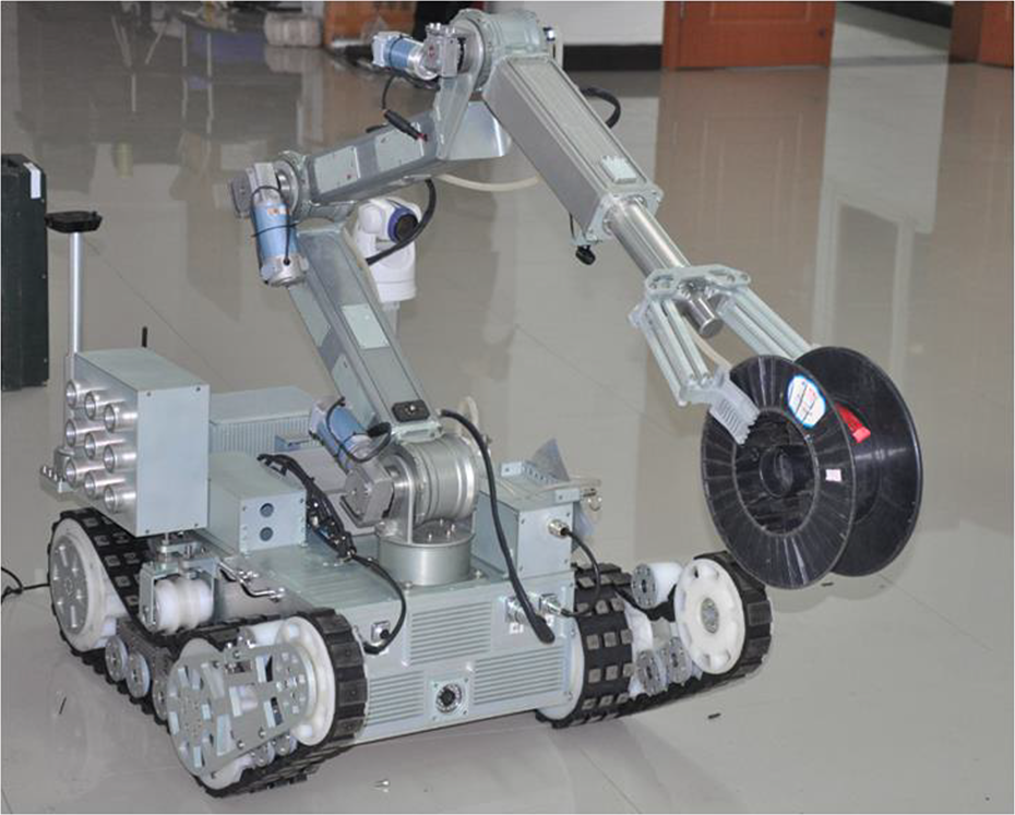
Actual image of a manipulator.

Simplified abstract model.
Kinematics and dynamics analysis of the manipulator
For the motion of a multi-joint manipulator, the transformation matrix between adjacent joints guides the kinematics and dynamics analysis and generally includes a rotation matrix and displacement. To standardize the rotation matrix and displacement vector, the initial position of the manipulator must be parameterized by the Denavit–Hartenberg (DH) method. The DH parameters of the manipulator are shown in Table 1.
DH parameters of the manipulator.a
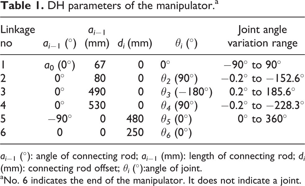
ai − 1 (°): angle of connecting rod; ai − 1 (mm): length of connecting rod; di (mm): connecting rod offset; θi (°):angle of joint.
aNo. 6 indicates the end of the manipulator. It does not indicate a joint.
The coordinate transformation of adjacent joints in the manipulator is generally denoted by

According to the theorem of inverse kinematics, there exists a solution to all joint angles when the axes of the three adjacent joints are parallel or orthogonal. When the three-dimensional (3-D) information of the end is fixed, eight groups of solutions can be obtained by inverse kinematics, as shown below

where tf is the termination time.
According to the Lagrange equation, the classical dynamics model of joints is deduced, as shown below

where
Optimal trajectory
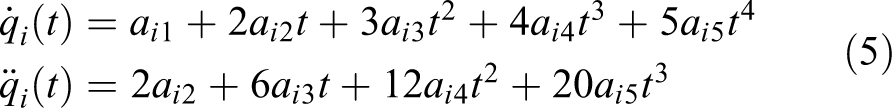
In this article, the trajectory of each joint is estimated by quantic interpolation, as shown below

Because angular velocity and acceleration are the first and second differentials of the angle, their formulas are shown below
Considering the objective facts of the starting and ending time of the manipulator, they are set as formula (6)

where t 0 is the starting time, and tf is the ending time.
Formulas (4) and (5) can be simplified as formula (7)

Formula (7) shows that the trajectory of each joint has three unknown coefficients, but only one final angle is known. The formula represents a mapping relationship from one variable to three variables. In this condition, the direct solution by the variation method leaves a set of 13 order equations with 15 unknown variables, with enormous computational complexity.
VGA-RBF model with the combined feedback control
A new method for solving the optimal control problem is proposed in this article. The method is called the variational method GA (VGA)-RBF model based on the combination feedback control. The VGA-RBF is a combination of the variation method, genetic algorithm, and radial basis function neural network. The method can be divided into three parts. The first part improves the accuracy of each joint by introducing a combination feedback control to control the closed-loop. The device compensates for the over-operation and under-operation of the joint. The second part provides the standard expected output for training samples according to solving the standard optimal trajectory curve by the variation method, laying the foundation for the next step of ANN training. In the third part, a fixed RBF neural network model is trained by the expected output provided by step two and training sample data. The GA is used to improve the generalization ability of the RBF network weights. The calculation process is fast, and the calculation results have good precision.
The system diagram of the algorithm is shown in Figure 3.

Algorithm system diagram.
Combined feedback control
To ensure reducing the overshoot of the manipulator’s path, feedback control of the angle, velocity, and acceleration is required for the optimal trajectory. The feedback control in this article combines linear and nonlinear feedback to improve the positioning accuracy at the end of the manipulator. 13 –18
Feedback control model
The dynamic model with feedback is shown in formula (8)

where
The feedback model

The space trajectory tracking of joints can be described as a limit problem of known reference input

where
The position error and velocity error are given in formula (11)

The feedback control is divided into linear and nonlinear feedback, as shown below


where Kp and Kd are i-order positive definite matrixes.

Q should satisfy below equation

To simplify the calculation, Kp , Kd , and Q are given. Kp and Kd are i × i known positive definite matrices. At the same time, Kp and Kd are diagonal matrices. Q is a 2i × 2i known positive definite matrix.
Proof of model stability
The stability of the feedback model is the basis for all subsequent work. Therefore, the model needs to prove the stability.
According to formula (9), the state equations are given below

where
According to formula (9), formula (17) is deduced
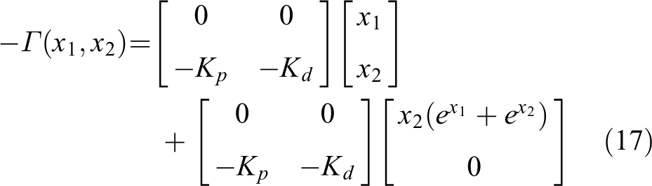
According to formulas (16) and (17), formula (18) is deduced

The Lyapunov function is defined by the following formula

P must be a positive definite matrix, so P≥0.
The derivation of the Lyapunov function of formula (19) is shown in formula (20)
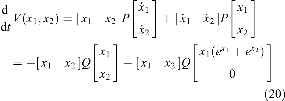
where
In conclusion,
Solution of the optimal trajectory by the variation method with feedback model
The variation method is a branch of mathematics developed at the end of the 17th century. The method belongs to the mathematical domain of processing functions and can be understood as a function of calculus. The variation method seeks the extremum function, which makes the functionals reach their maximum or minimum values. 19 –22
State equations of the manipulator
According to sections Combined feedback control and Solution of the optimal trajectory by the variation method with feedback model, the state variables are set according to the below formula

The state equations are shown below

Optimal control model based on the variation method
Optimal objective functions are first needed when solving the optimal trajectory. Time optimal and energy optimal are the two objectives selected in this article, as shown below


These two optimal indexes are combined to obtain the comprehensive optimal index, as shown below

The optimal objective function is obtained based on formulas (23) and (24), as shown below

The Hamiltonian function is constructed according to the optimal solution of the variation method, as shown below

The co-state equations and state equations are constructed according to the Hamiltonian function, as shown below


Optimal trajectory of the manipulator solved by the GA-RBF method
In this article, a method is presented to simply and conveniently solve the optimal trajectory. While each DOF has only one angle, each DOF in the optimal trajectory needs three coefficients, which leads to a mapping problem from low-dimensional input to high-dimensional output, where the trained neural network can solve the complex computation and find a nonunique solution. The RBF network is a neural network 23 –25 that regards the RBF as the “base” of the hidden units forming the hidden layer space so that the input vector can map directly to the hidden space without weight connection. According to Cover’s theorem, the hidden layer of the RBF can map the input of low-dimensional space to high-dimensional space via a nonlinear function. This high-dimensional space can fit the curve. This process is equivalent to finding a surface that can best fit the training data in a hidden high-dimensional space, which is different from the ordinary MLP. In the RBF neural network, the initial weights are often given randomly. This situation may seriously affect the learning efficiency, so the GA is introduced to obtain the initial weights in this article, which improves the training efficiency and prediction accuracy of the neural network. 26 –28
RBF neural network
The structure of the RBF network is a three-layer forward network similar to that of the multilayer forward network. The first layer is the input layer, which consists of a signal source node. The second layer is the hidden layer. The number of hidden units depends on the needs of the problem, and the transformation function of the hidden units is an RBF that is nonnegative, nonlinear, symmetric, and attenuated for the center point. The third layer is the output layer, which responds to the input mode. The transformation from the hidden layer to the output layer is linear, while the transformation from the input space to the hidden layer space is nonlinear. The net topology of the RBF neural network is shown in Figure 4.

Topology of the RBF neural network. RBF: radial basis function.
The number of nodes in the network’s input layer is determined by the data dimension of the input signal. The hidden layer is between the input layer and the output layer, and the data of the hidden layer are a set of RBFs derived from the input data. Generally, the Gauss function is used as the calculation method of the RBF. The data output from the hidden layer to the output layer follows the principle of weighted superposition as the output data of the RBF network. In this article, the RBF neural network is studied the regularization. The numbers of nodes in the input layer, hidden layer, and output layer are N 1 = 5, N 2 = 5, and N 3 = 15, respectively. If the input is [q1, q2, q3, q4, q5 ] T , the output of the jth neuron in the hidden layer is given below

where
The convergence step of the network is shown below

where P is the number of samples.
According to the least mean squares algorithm, the weight of the formula can be adjusted below

where W is the weight matrix from the hidden layer to the output layer, η is the learning speed, and Φ is a vector of hidden nodes.
The output data for each neuron in the output layer is given below

where wjk , which is an N 2 × N 3 matrix, represents the connection weights of each node from the hidden layer to the output layer.
Optimal weight matrix by GA
The GA method, which was proposed by Holland in the 1960s,
29
can optimize the weight matrix from the hidden layer to the output layer in the RBF neural network. The GA is a random search method based on natural selection and genetic mechanisms. The GA search begins with the coding group of the solution. The GA searches for information on the basis of a fitness function and does not require a derivative or other information. Moreover, the GA converges to the global optimal solution with probability 1. In this article, the GA method is selected to calculate the weight matrix from the hidden layer to the output layer. The weight matrix is based on data samples in the RBF networks and is obtained via the following main steps. 1. A set of weights from the hidden layer to the output is first generated randomly. Each row in the N
2 × N
3 matrix is regarded as a population, and each element is regarded as an independent entity in the corresponding population. 2. The encoding of each individual obeys rules with a step size of 0.1 from 0 to 1. The sum of the 15 elements in each line is 1. 3. According to the sample input, the fitness function is established, as shown below

where f is the fitness. Q is the input vector, W is the weight matrix, and
4. The RBF network is continuously inherited and undergoes mutation according to the fitness function. When the fitness is reduced, the result of the genetic coding is inherited; conversely, when the fitness increases, the result of the genetic coding is changed.
Experiments
For the KUKA manipulator, positive kinematics can solve the scope of the manipulator’s movement. The range of motion is shown in Figure 5. Figure 5(a) shows the range of motion in the two-dimensional plane, and Figure 5(b) shows the range of motion in the 3-D plane.

Sketch of the end range of motion. (a) 2-D plane with the x- and y-axes. (b) 3-D plane with the x-, y-, and z-axes. 3-D: three-dimensional; 2-D: two-dimensional.
A total of 10,000 points evenly grid the end range of motion with its 3-D information. This 3-D information can solve the eight groups of solutions by inverse kinematics for each point. According to the constraints and the actual situation of each joint, the unique solution of each point is obtained, as shown in Table 2.
3-D information and angles for 10,000 points.

3-D: three-dimensional.
The first group of data is regarded as an example. The optimal trajectory parameters of each joint are shown in Table 3.
The optimal trajectory parameters of the first group.

The first 9000 groups of data are training samples, and the remaining 1000 groups of data are testing samples. The test environment is a PC with 16 GB memory and a 1.8 GHz × 4 CPU. The following section presents the details of the experiment.
Impact on the results with and without the feedback control
To further improve the accuracy of the neural network algorithm, the final result of the testing samples is returned to the feedback system along with its joint angle error, as shown in Figure 6.

The angle error of each joint under conditions with and without feedback.
In Figure 6, red represents the error range with feedback. The average accuracy of the angle is increased by 51.6% when feedback is included. In this condition, the error range converges from −2° to 2°. This level of accuracy satisfies the requirements of the manipulator.
Similarly, the errors between the sum of the joint torques and the theoretical values are compared in the two conditions. The comparison results are shown in Figure 7.

The error between the sum of the joint torques and the theoretical values.
The experiment shows that the sum of the minimum torques obtained by our method is almost equal to the theoretical values. The accuracy without feedback reaches 98.1%, and the accuracy with feedback reaches 99.3%. These results confirm the solution to the optimal trajectory obtained by the RBF neural network with feedback.
The results prove that the method in this article is correct and useful. Via feedback control, the output information of the system is returned to the input, and the output information is compared with the input information. Deviations between the input and output are used for control; hence, feedback is very important.
Comparison of different feedback controls
Table 4 compares three conditions: combined feedback, linear feedback, and nonlinear feedback. Under these conditions, we calculate the angular errors of five joints and the error variance of 1000 testing samples.
Comparison of three feedback controls.
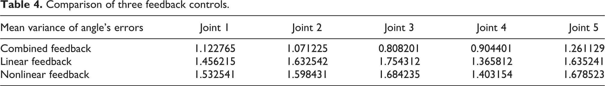
Table 4 shows combined feedback outperforms in terms of accuracy because the combination of linear and nonlinear characteristics can accurately describe the system. The average error of each joint is reduced by 0.4°.
The results show that the method in this article is correct and useful. The proposed feedback control satisfies the requirements by providing linear feedback and nonlinear feedback. For example, the error produced by continuous operation of the motor is linear error, and the error caused by the time difference between starting and braking is nonlinear. This feedback provides good compensation for joint angle control.
Comparison of different methods of solving the expected output
Table 5 shows the operation time and energy consumption for the variation method and other methods. The values in Table 5 are the averages of 1000 groups.
Comparison of optimal control.

DMOC: Discrete mechanics and optimal control.
Table 5 shows that the variation method is the best. The operation time is reduced by 2.31%, and the energy consumption is reduced by 2.15%.
The results show that the method in this article is accurate and useful. Optimal control is a control function that solves the performance index to a certain extreme value under specific conditions. Mathematically, optimal control is a conditional extremum problem for finding a functional under the constraint of a differential equation, which is simply a variational problem. Therefore, the variational method is a suitable way to solve the problem.
Comparison of different ANN methods
Table 6 compares the RBF and MLP (one layer, two layers, three layers, and four layers) experiments. The error and operation time of the 15 parameters are compared.
Comparison of different neural network methods.

RBF: radial basis function; MLP: multilayer perceptron.
In Table 6, the operation time of RBF is the second shortest, and its accuracy is the highest among the five methods. Therefore, the RBF ensures both efficiency and accuracy.
The results show that the method in this article is correct and useful. The characteristics of RBF global optimization are fully reflected. The reduction in error proves that some values are locally optimal.
Comparison of GA-RBF and RBF
The training and testing samples are input into the RBF network and the GA-RBF network, respectively. Figure 8 shows the angular acceleration curve of each joint. Figure 9 gives the angular velocity curve of each joint. Figure 10 shows the angle curve of each joint.
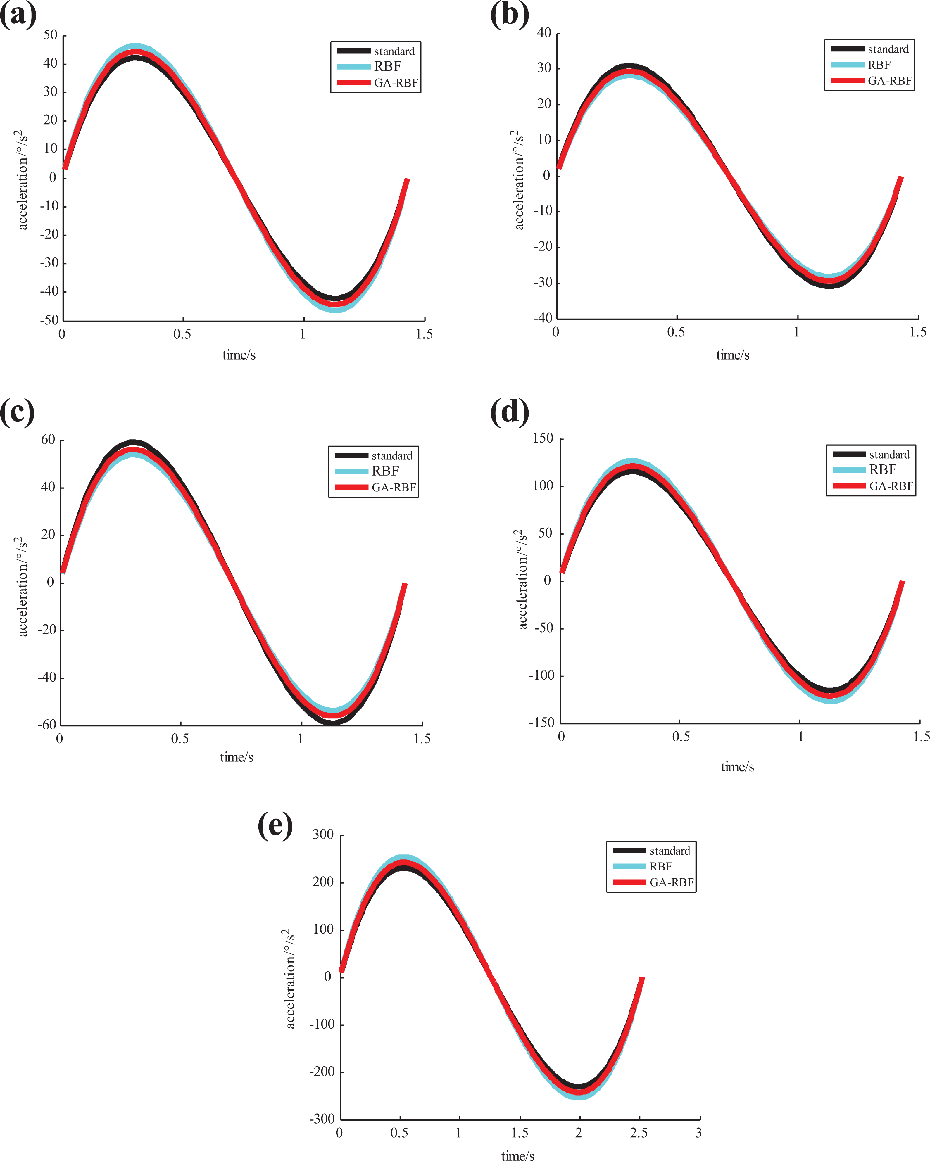
Angle acceleration curve of each joint: (a) angle acceleration curve of joint 1, (b) angle acceleration curve of joint 2, (c) angle acceleration curve of joint 3, (d) angle acceleration curve of joint 4, and (e) angle acceleration curve of joint 5.

Angle velocity curve of each joint: (a) angle velocity curve of joint 1, (b) angle velocity curve of joint 2, (c) angle velocity curve of joint 3, (d) angle velocity curve of joint 4, and (e) angle velocity curve of joint 5.

Angle curve of each joint: (a) angle curve of joint 1, (b) angle curve of joint 2, (c) angle curve of joint 3, (d) angle curve of joint 4, and (e) angle curve of joint 5.
In Figures 8 to 10, the black curve is the standard value, the blue curve is the value obtained by the RBF method, and the red curve is the value obtained by the GA-RBF method. The curve from the neural network fluctuates around the standard data and is basically in accordance with the standard values. The results prove that the method is effective. For 1000 groups of testing samples, the average error curve of the 15 parameters in Figure 11 is obtained accurately and quickly.

Average error of the 15 parameters for the testing sample.
In practice, the operation time for 1000 samples is 7.378 s for the RBF neural network. In the GA-RBF neural network, the time consumed for 1000 samples is 7.382 s, while the traditional method requires 58.635 s. In this article, the computational efficiency is much better than that of the traditional algorithm. The accuracy of the GA-RBF algorithm is improved by 18.62% compared with that of the RBF algorithm. Although the accuracy of the neural network is reduced, the average error is still less than 3.5. The parameters are converted into curves, which fluctuate around the standard curve. The calculation of the angle, angular velocity, and acceleration has little effect.
The results proved that the method in this article is correct and useful. GA is introduced to obtain the initial weights. The initial weights of the RBF are not randomly assigned, and the initial weights improved by the GA affect the learning efficiency. Therefore, the proposed method can improve the training efficiency and prediction accuracy of neural networks.
Conclusions
In this article, a method for solving the optimal trajectory of a five-DOF open chain link manipulator is presented. The experiment proves that the method is effective with 10,000 samples. The main conclusions are as follows: The feedback control can provide effective compensation for joint over-operation and under-operation, thereby improving the accuracy of each joint angle. The RBF neural network improved by GA has a distribution of weights that is closer to the actual situation. In practice, the calculation is performed in a trained neural network, so the operation time is improved.
The method in this article can find the optimal trajectory with the optimal operation time and energy consumption. The method also outperforms in terms of accuracy, which is of great significance for engineering.
Footnotes
Declaration of conflicting interests
The author(s) declared no potential conflicts of interest with respect to the research, authorship, and/or publication of this article.
Funding
The author(s) disclosed receipt of the following financial support for the research, authorship, and/or publication of this article: This work was partially supported by Beijing Natural Science Foundation with No. 4192042, National Science Fund subsidized project with No. 61627816, and Beijing Science and Technology Plan Project with No. D161100004916002.