Sage Journals: Discover world-class research

Abstract

In the development of autonomous driving, decision-making has become one of the technical difficulties. Traditional rule-based decision-making methods lack adaptive capacity when dealing with unfamiliar and complex traffic conditions. However, reinforcement learning shows the potential to solve sequential decision problems. In this article, an independent decision-making method based on reinforcement Q-learning is proposed. First, a Markov decision process model is established by analysis of car-following. Then, the state set and action set are designed by the synthesized consideration of driving simulator experimental results and driving risk principles. Furthermore, the reinforcement Q-learning algorithm is developed mainly based on the reward function and update function. Finally, the feasibility is verified through random simulation tests, and the improvement is made by comparative analysis with a traditional method.

Keywords

Automatic driving decision-making algorithm Markov decision process reinforcement Q-learning

Introduction

In recent years, decision-making has been regarded as a core technology when dealing with vehicle longitudinal automatic driving problems. However, a feature of vehicle longitudinal automatic driving is car-following, which represents the most common phenomenon in real traffic environments.

A vehicle longitudinal automatic driving system is divided into three parts: environmental perception, decision-making, and control execution. Among these parts, environment perception and control execution are relatively mature and have achieved good results by the research of experts.¹ For example, Gao et al.² put forward an object classification method based on a convolutional neural network and image upsampling theory to obtain informative feature representation in an autonomous vehicle environment using integrated vision and light detection and ranging data. Hence, he established a trajectory prediction model combined with physics- and maneuver-based models to solve nonlinear estimation and prediction problems, and this interactive multiple model trajectory prediction approach could predict more accurately than the single model.³

In addition, there is still room for decision-making improvement. Compared with a traditional rule-based decision-making method, an independent decision-making method can transform a decision mechanism, as shown in Figure 1.

Figure 1.

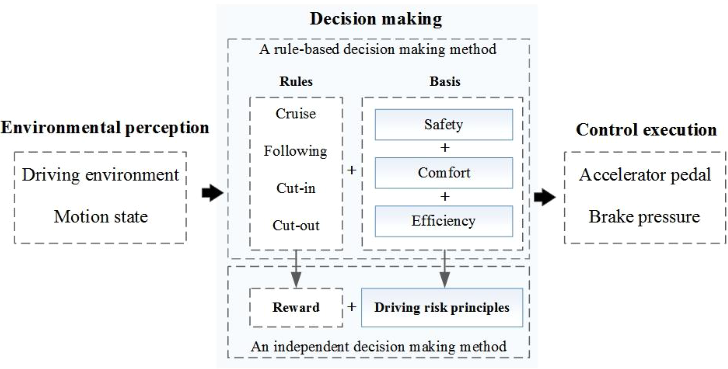
A comparison of two decision-making mechanisms.

In Figure 1, the function of decision-making is to convert the environmental information to an action command. That is, the environmental perception part will provide the environmental information for decision-making, and the control execution part will convert an action command to a specific control signal. If we regard the environmental perception part as human eyes and ears and regard the control execution part as human hands and feet, the decision-making part is much like a human brain.

Therefore, the key technology of decision-making is an independent decision process that imitates that mechanism in humans.

Preliminary studies have shown that traditional decision-making methods are mostly based on tedious indicators of safety, comfort, and efficiency, which are generally established with rules to realize a dynamic decision.⁴ Traditional methods can match most driving situations but lack adaptive capacity when faced with unpredictable and complex traffic conditions. However, some emerging machine learning algorithms, such as the current popular “end-to-end” method, are so empirical that they mostly rely on probabilistic reasoning but ignore the causal relationship between the current state of the vehicle and the action performed.

At present, to solve the above problems, experts hope to improve this causality when an independent decision is made during vehicle longitudinal driving. Hence, reinforcement learning has shown the potential to solve cause-and-effect reasoning problems in recent years. For example, Vanderhaegen and Zieba⁵ realized the prediction of the driver’s expected action by designing prefeedback action and postfeedback knowledge controllers and using a consolidated and accumulated reinforcement learning algorithm. Desjardins and Chaib-Draa⁶ utilized learning algorithms of approximation and gradient descent to realize the queue control of vehicles and optimized its consistency. Rui⁷ applied a reinforcement learning algorithm in a decision-making layer design for autonomous highway driving, and this algorithm enabled the vehicle to acquire the correct decision through interactive online learning with the environment. Chunming⁸ proposed a basic framework for solving multiobjective reinforcement learning problems and optimized a longitudinal automatic control algorithm in the continuous state space of vehicle motion, but the final learning results lacked drivers’ own driving behavioral characteristics due to different learning objects and methods. Instead, some scholars have used real driver experimental data to simulate drivers’ following features. For example, Chong et al.⁹ utilized data of drivers’ own characteristics, the relative motion relationship, and environmental factors as system inputs. They established a driver model on the basis of a fuzzy nerve network, and this model imitated driving characteristics during vehicle longitudinal automatic control.⁹ Li and Gao¹⁰ designed a decision-making module as a driving brain associated with a sensor information-processing module, and the designed module reduced the impact of changes in sensor quantity, types, and installation locations on the entire software framework.

By analyzing the above results, it is not difficult to find that traditional rule-based methods are applicable but lack adaptive capacity due to their inherent logic switching strategy. Therefore, based on previous studies, in this article, we propose an independent decision-making method with a causal reasoning mechanism based on a reinforcement learning algorithm to improve flexibility and adaptivity. The contribution of this article is briefly described as follows: (1) A traditional rule-based decision-making method is replaced by an independent decision-making method. (2) A Markov decision process (MDP) model is established by analysis of car-following. (3) Driving simulator experiments and driving risk principles are provided for the design of the algorithm. (4) A reinforcement Q-learning algorithm is developed mainly based on the design of the reward function and the update function. (5) The feasibility is verified through random simulation tests. (6) Improvement is made by comparative analysis with the traditional method.

The remainder of this article is organized as follows: The second part is “MDP modeling for car-following.” The third part is “Driving simulator experiment.” The fourth part is “Reinforcement Q-learning,” including the state set, action set, reward functions, and update function. The fifth part is “Simulation tests,” and the final part is “Conclusions and future work.”

MDP modeling for car-following

Independent decision-making is regarded as a complex sequential decision problem. Although it is difficult to break down these problems through traditional fuzzy classification or rule-based modeling, in the field of probability and statistics, an MDP provides a mathematical model for solving a decision-making problem, even if the problem is partly random or partly controlled by humans.

When dealing with MDP problems, we use a preliminary instruction: a Markov process (MP) and a Markov reward process (MRP). The MP is a Markov process with a Markov property, which means the conditional probability of the process is only related to the current state of the system and is independent and irrelevant to its past history and future state. The MRP is a Markov process with a reward, and this process can be represented by four elements: S represents a finite set of states, P represents a state transition matrix, R represents a reward, and $γ \in [0, 1]$ represents a discount factor. Therefore, the MDP is developed from the MRP when considering a decision, such as a specific action. Table 1 presents the construction elements of the MDP model.

Table 1.

MDP elements.

	Element	Symbol
1	State set	S
2	Action set	A
3	State transition probability	P_sa
4	Damping coefficient	$γ \in [0, 1)$
5	Reward function	R

MDP: Markov decision process.

In addition to the above elements, three core concepts need to be illustrated: (1) policy, (2) reward, and (3) value function.

Policy

The policy “π: S → A” represents the way for the agent (vehicle) when selecting an action. When the vehicle interacts with the traffic environment, the policy π indicates that the vehicle can output a certain action from action set A at the moment of current state S.

Reward

The reward indicates the immediate assessment of the environment when selecting an action. The reward maps the current state of the environment to a return signal r, which is often defined as a scalar (e.g. a positive number for a reward and a negative number for punishment).

Value function

The value function refers to the accumulation of immediate rewards and reflects good or poor behavior for a long time. A final action is selected on the basis of the largest value function. Thus, we consider a series of actions’ reward $V^{π} (s)$ under policy π, as shown in equation (1)

V^{π} (s) = r_{t} + γ r_{t} + γ^{2} r_{t} + \dots = \sum_{i = 0}^{\infty} γ^{i} r_{t + 1}

When $V^{π} (s)$ is at its maximum, policy π becomes an optimal policy “ $π^{*}$ ,” as shown in equation (2)

π^{*} (s) = {arg}_{a} max [r (s, a) + γ V^{*} (δ (s, a))]

After building an MDP model, we need to solve the model through an algorithm. As mentioned before, reinforcement learning shows the potential to solve cause-and-effect reasoning problems and is an effective method for solving the model. For example, a “dynamic programming (DP)” algorithm uses the value function to search for a good policy, which requires all accurate dynamic information of the external environment, and the value iteration calculation is large. A “Monte Carlo (MC)” algorithm is adopted to conduct simulation experiments, collect data, and calculate average cumulative returns through an interactive evaluation value function with the environment. As a fusion of DP and MC algorithms, a temporal difference algorithm, which is difficult to develop and apply in engineering, updates the value function in accordance with two successive prediction errors. In addition to the general algorithms above, a Q-learning algorithm improves the traditional iterative problem and translates the original complex decision-making problem into a process of using a Q-table.^11
–13 However, the core of the Q-learning algorithm is determining how to estimate the value function effectively.

As a result of the limited training sample, no (s, a) exist in any reality. Thus, an intelligent agent cannot learn an optimal policy π*(s) or obtain perfect knowledge of the state transition probability and reward function.^14,15 Therefore, we attempt to transform value function V(s) to evaluation function Q(s, a) associated with action a when addressing the MDP problem, as shown in equations (3) and (4)

Q (s, a) = r (s, a) + γ V^{*} (δ (s, a))

π^{*} (s) = {arg}_{a} max Q (s, a)

We assume that the vehicle is in a certain state “s” of state set S and successively calculates the cumulative return corresponding to all actions in action set A on the basis of a greedy strategy. The corresponding actions are selected in accordance with the maximum Q-value, and the current state is executed and updated, as shown in Figure 2.

Figure 2.

One-step state transfer process.

Driving simulator experiment

Because a real driving experiment may require a large amount of time and financial resources, we chose to build a driving simulator for different drivers with different styles.

As shown in Figure 3, the state and action sets required for algorithm construction were mostly based on artificially set ranges in previous studies.¹⁶ Instead, we tried to make the algorithm cover as many complex driving conditions as possible, and we attempted to conduct the same experiment for different types of drivers.¹⁷ Thus, we established a unified driver experimental database with speed, relative distance, and acceleration.

Figure 3.

Driving simulator experimental data: (a) aggressive driver, (b) conventional driver, and (c) conservative driver.

Reinforcement Q-learning

In view of the core technical problem of vehicle longitudinal automatic control, traditional vehicle factories basically adopt decomposed design through the following aspects: environmental perception, decision-making, and control execution; however, some emerging Internet companies are more likely to use “end-to-end” designs. Either way, these approaches will increasingly rely on machine learning techniques.

Compared with other machine learning algorithms, a reinforcement Q-learning algorithm transforms the decision value function V(s) related to the state into evaluation function Q(s, a) related to the action for calculation according to equations (3) and (4). Therefore, the optimal action sequence can be selected only by calculating the Q-value in the current state.

The state set and the action set

When making a behavioral decision in the practical driving process, the principle of selecting the state set is to use as few major states as possible to represent the actual state. The initial state set consists of vehicle motion state information obtained using the driving simulator, such as velocity, acceleration, and relative distance. However, this state set may contain too much redundant information, such that the state characteristics are not evident. Therefore, in this study, the initial driving state set is processed based on driving risk principles, and this process evaluates drivers’ current driving status and reflects their understanding of the current driving environment. Research on driving risk has shown¹⁸ that the driver mainly focuses on two aspects: (1) driving safety and (2) driving efficiency.

Driving safety is affected by two factors: velocity and relative distance. Numerous studies have shown¹⁹ that driving safety decreases with increasing speed and increases with increasing distance. However, when the speed is not higher than the average speed, the gradient change will not affect the driving safety. In addition, the driver’s incorrect assessment of relative distance will cause driving risk.

Psychological research results indicate²⁰ that in the driving process, the driver always expects to reach the expected destination with the fastest speed. This relatively fast speed is called the expected speed. For different drivers, the expected speeds vary. However, the higher the expected speed is, the higher the driving efficiency.

The driver will perform a series of actions to change the relative motion state of the vehicle when following. To facilitate the convergence of the learning process and simplify the model, the final state set and action set are designed by considering the above principles, as shown in Figure 4.

Figure 4.

The state set and the action set in the design of reinforcement Q-learning.

Reward functions

The purpose of an independent decision-making algorithm is to make the vehicle generate an action instruction in accordance with the current state information and maximum future total reward. The ultimate effect is the dynamic control of the safety distance between vehicles. Therefore, the reward functions should reflect the relative motion relationship between vehicles and the dynamic characteristics of vehicles, as shown in Figure 5 and Table 2.

Figure 5.

Safety distance model when following.

Table 2.

Parameters in Figure 5.

Symbol	Variable	Unit
Vx	Current speed of ego vehicle	m/s
D	Current relative distance	m
Vr	Current relative speed	m/s
Ax	Current acceleration of ego vehicle	m/s²
V_set	Set expected speed	m/s
D_set	Set expected distance	m
Vx1	Next speed of ego vehicle	m/s
D1	Next relative distance	m
Vr1	Next relative speed	m/s
A	Next acceleration of ego vehicle	m/s²

If the sampling interval is 0.01 s, then a possible action is decided every 0.01 s in the current state. Thus, the relationship between the current motion state and the next motion state can be described by equation (5)

{\begin{matrix} V x 1 = V x + A x \times t \\ D 1 = D + V r \times t \\ V r 1 = V r + A x \times t \end{matrix}

According to equation (5), we can obtain the target vehicle’s motion state by calculating the relative speed: (1) if the target vehicle is accelerating, then we do not need to consider the relative distance because there is no possibility of collision and (2) if the target vehicle is decelerating, then we must consider the relative distance.

As mentioned above, we have to consider different motion states of the target vehicle. Therefore, the reward functions need to contain two types: an acceleration reward function “ $r^{+}$ ” and a deceleration reward function “ $r^{-}$ ”.

When the target vehicle is accelerating, the ego vehicle should theoretically make a decision to accelerate and ultimately reach the same speed as the target vehicle. Thus, if the next speed Vx1 ∈ [0, 30] m/s, then we determine the relation between Vx1 and the current speed Vx. Reward function r1 is shown in equation (6)

r 1 = {\begin{matrix} 10 V x 1 > V x \\ - 10 V x 1 < V x \end{matrix}

First, if the next speed is larger than the current speed ( $V x 1 > V x$ ), then the vehicle is accelerating with a reward of 10. If the next speed is smaller than the current speed ( $V x 1 < V x$ ), then the vehicle is decelerating with a punishment of −10.

Next, we make a further contrast between Vx1 and V_set. Then, we can obtain the reward function r2, as shown in equation (7)

r 2 = {\begin{array}{l} 100 & Δ V > 0 or Δ V < 0.5 \\ - 1 & Δ V \geq 0.5 \end{array}

where $Δ V = V_s e t - V x 1$ represents the difference between the expected speed and the next speed.

Finally, the acceleration reward function is shown in equation (8)

r^{+} = {\begin{array}{l} r 1 + r 2 & V x 1 \in [0, 30] \\ - | Δ a | & V x 1 > 30 \end{array}

where $Δ a = A - A x$ indicates the difference between the next acceleration and the current acceleration.

When the target vehicle is decelerating, the ego vehicle should theoretically make a decision to decelerate and ultimately reach the same speed as the target vehicle.

First, if the next speed Vx1 ∈ [0, 30] m/s, then we divide the reward function into three aspects, which represent different degrees of emergency: (1) near mode, with a reward of 100; (2) dangerous mode, with a punishment of −1; and (3) emergency mode, with a reward of 10, as shown in equation (9)

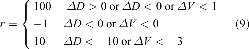
r = {\begin{array}{l} 100 & Δ D > 0 or Δ D < 0 or Δ V < 1 \\ - 1 & Δ D < 0 or Δ V < 0 \\ 10 & Δ D < - 10 or Δ V < - 3 \end{array}

Among these aspects, $Δ D = D_s e t - D 1$ indicates the difference between the expected distance and the next distance.

Next, if Vr1 < 0, then ΔV represents the difference between the expected speed and the next speed; if Vr1 > 0, then ΔV represents the opposite of Vr1.

Finally, the deceleration reward function is shown in equation (10)

r^{-} = {\begin{array}{l} r & V x 1 \in [0, 30] \\ - | Δ a | & V x 1 > 30 \end{array}

where $Δ a = A - A x$ indicates the difference between the next deceleration and the current deceleration.

Update function

The process of reinforcement learning is a continuous state update process.

In each learning period, the system will randomly figure out a certain action based on the greedy algorithm to generate an immediate reward. However, as mentioned before, the value function is the Q-value of the updating function. Therefore, the system can calculate the total reward by iteration based on the updating function.

Finally, the system will perform an action specifically according to the maximum value of the total reward. Figure 6 shows the Q-value updating process.

Figure 6.

Q-value updating process.

At the beginning, the system will generate an empty Q-table, which includes a pair of “state-action” corresponding to the Q-value. Thus, the learning process becomes an updating process with Q-values. Then, the calculation of the Q-value with policy π is shown in equation (11)

V^{π} (s) = r_{t} + γ r_{t} + γ^{2} r_{t} + \dots = \sum_{i = 0}^{\infty} γ^{i} r_{t + 1}

where the maximum of $V^{π} (s)$ corresponds to the optimal policy “ $π^{*}$ ,” as shown in equation (12)

π^{*} (s) = {arg}_{a} max [r (s, a) + γ V^{*} (δ (s, a))]

where γ ∈ [0, 1] represents the discount factor, which indicates how important future returns are relative to current returns. If γ = 0, then the function considers only immediate returns but not long-term returns. If γ = 1, then the function regards the immediate and long-term returns as coequal. Hence, we tend to transform V(s) into Q(s, a), as shown in equation (13)

Q (s, a) = r (s, a) + γ V^{*} (δ (s, a))

In this way, we can obtain the Q-value function with policy π when selecting an action “a” at state “s,” as shown in equation (14)

Q^{π} (s, a) = E_{π} {\sum_{k = 0}^{\infty} γ^{k} r_{t + k + 1} | s_{t} = s, a_{t} = a}

According to the Bellman equation, we can convert equation (14) to equation (15)

Q^{π} = E_{π} {r_{t + 1} + γ \sum_{k = 0}^{\infty} γ^{k} r_{t + k + 2} | s_{t} = s, a_{t} = a}

Equation (15) indicates the relationship between the current state value and the next state value. Thus, according to the Bellman equation, we will obtain the optimal policy value function $Q^{*} (s, a)$ , as shown in equation (16)

Q^{*} (s, a) = max Q^{π} (s, a)

When the current state changes to the next state, we regard the next state as the current state and record it. Thus, the vehicle executes an action and performs cycling to continue the process. Therefore, the update function of the Q-table is shown in equation (17)

Q (s, a) \leftarrow Q (s, a) + α [r + γ max Q (s^{'}, a)]

As each step of the state transfer is accompanied by the selection of actions, this selection can be performed successively in an iterative manner through local optimization to achieve the overall optimal decision scheme. Thus, we use the policy of the greedy strategy, which can explore on the basis of “ε” and develop on the basis of “1 − ε.” In addition, “ε” often has a small value of 0.01, such that the algorithm can be used to select the optimal action with a probability of approximately 1.

Simulation tests

First, a vehicle longitudinal automatic driving model is established Matlab [version 2016b] with Simulink. Then, a series of random driving conditions are designed through CarSim [version 2016.1] to verify the feasibility. Finally, a comparative analysis is made between the proposed method and a traditional method.

As shown in Figure 7, environmental perception is a module that provides vehicle motion information, such as velocity, acceleration, relative distance, and relative velocity. Decision-making is a module that outputs action signals based on the reinforcement Q-learning algorithm according to the vehicle motion information. Control execution is a module that converts an action signal to a specific control command. In addition, the parameters of the vehicle can be adjusted through the vehicle model in CarSim.

Figure 7.

Construction of the simulation model based on Simulink and CarSim.

Constant speed tests

In this part, we assume that the target vehicle is driving at a constant speed. Hence, three different driving conditions, “following,” “cut-in,” and “cut-out,” are considered for low speed (40 km/h), medium speed (80 km/h), and high speed (120 km/h) of the target vehicle.

The simulation results for the target vehicle driving at a low speed of 40 km/h for 100 s are shown in Figure 8. The relative distance is approximately 20 m, and the speed of the ego vehicle is approximately 40 km/h at the beginning. The desired speed and the relative distance are 40 km/h and 20 m, respectively. The target vehicle cut-out from the original lane at 25 s and cut-in at 60 s.

Figure 8.

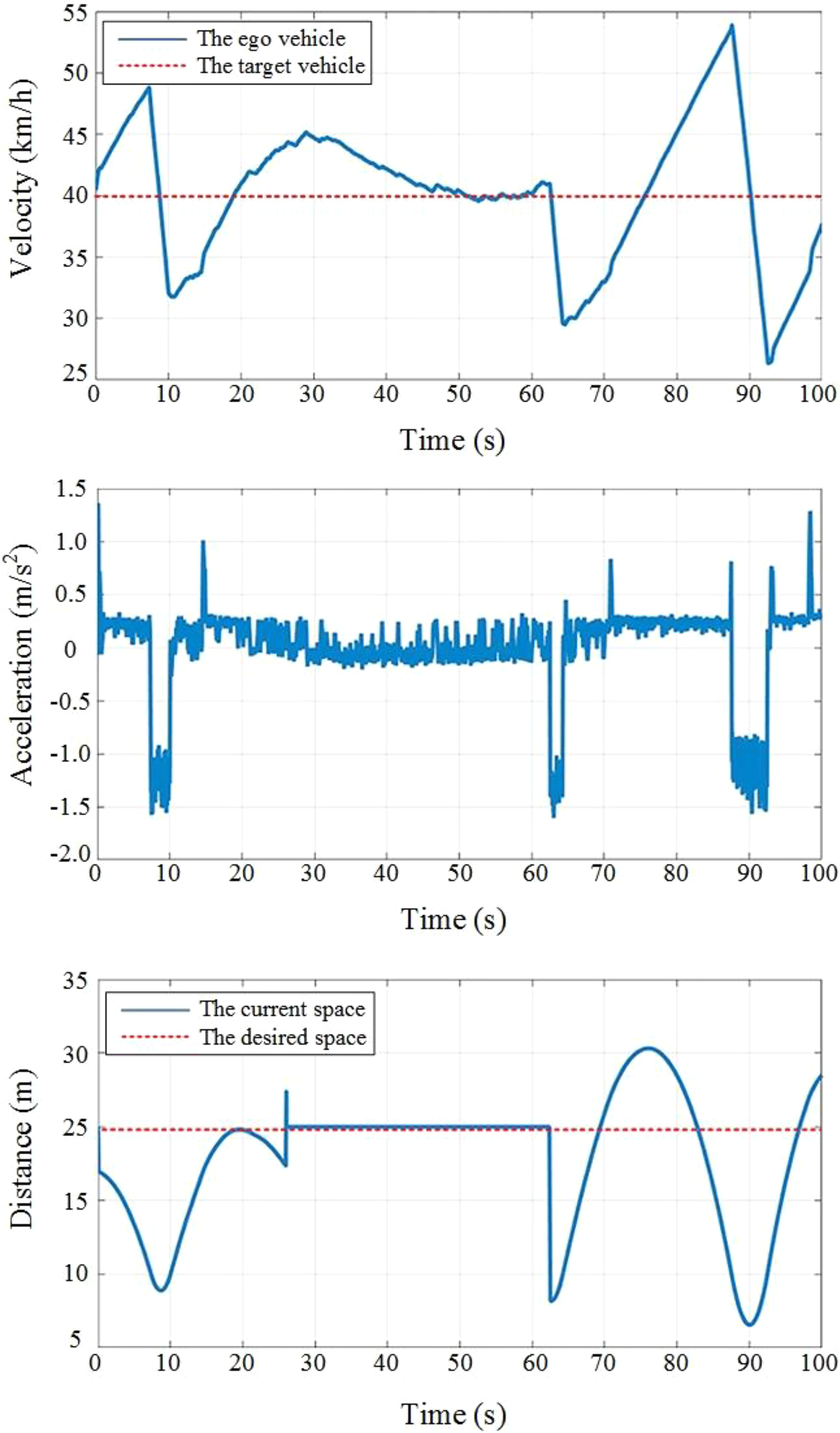
The simulation results for the target vehicle driving at a constant low speed.

The simulation results for the target vehicle driving at a medium speed of 80 km/h for 100 s are shown in Figure 9. The relative distance is approximately 20 m, and the speed of the ego vehicle is approximately 80 km/h at the beginning. The desired speed and the relative distance are 80 km/h and 20 m, respectively. The target vehicle cut-out from the original lane at 50 s and cut-in at 70 s.

Figure 9.

The simulation results for the target vehicle driving at a constant medium speed.

The simulation results for the target vehicle driving at a high speed of 120 km/h for 100 s are shown in Figure 10. The relative distance is approximately 50 m, and the speed of the ego vehicle is approximately 120 km/h at the beginning. The desired speed and relative distance are 100 km/h and 500 m, respectively. The target vehicle cut-out from the original lane at 15 s, cut-in at 20 s, and cut-out at 50 s.

Figure 10.

The simulation results for the target vehicle driving at a constant high speed.

Variable speed tests

In this part, we assume that the target vehicle is driving with variable speed. Hence, three different driving conditions, “following,” “cut-in” and “cut-out,” are considered for low speed (speed limit of 40 km/h), medium speed (speed limit of 80 km/h), and high speed (speed limit of 120 km/h) of the target vehicle.

For the target vehicle driving at an initial speed of 40 km/h, the following random driving conditions are shown in Figure 11. The ego vehicle is driving at a speed of 60 km/h, and the desired speed is 20 km/h. The desired and relative distances are both 80 m. The target vehicle cut-out at 60 s and cut-in at 70 s. The simulation results are shown in Figure 12.

Figure 11.

The random driving conditions of the target vehicle with a speed limit of 40 km/h.

Figure 12.

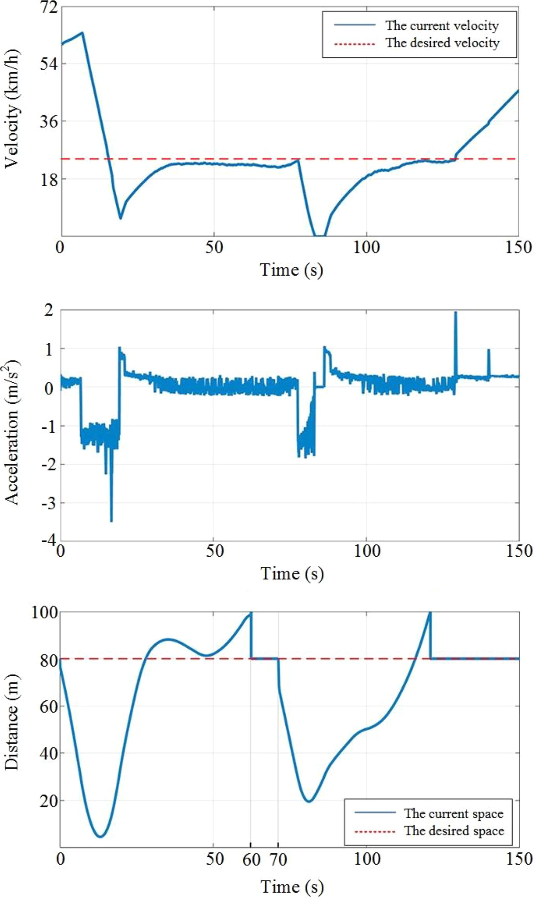
The simulation results for the target vehicle driving with variable low speed.

For the target vehicle driving at an initial speed of 60 km/h, the following random driving conditions are shown in Figure 13. The ego vehicle is driving at a speed of 70 km/h, and the desired speed is 40 km/h. The desired distance is 50 m, and the relative distance is 20 m. The target vehicle cut-out at 20 s and cut-in at 27 s. Moreover, the target vehicle is beyond the default radar detection range at 42 s but is restored at 70 s, as shown in Figure 14.

Figure 13.

The random driving conditions of the target vehicle with a speed limit of 80 km/h.

Figure 14.

The simulation results for the target vehicle driving with variable medium speed.

For the target vehicle driving at an initial speed of 80 km/h, the following random driving conditions are shown in Figure 15. The ego vehicle is driving at a speed of 100 km/h, and the desired speed is 80 km/h. The desired distance is 50 m, and the relative distance is 20 m. The target vehicle cut-out at 3 s and cut-in at 8 s. Moreover, the target vehicle is beyond the default radar detection range at 98 s, as shown in Figure 16.

Figure 15.

The random driving conditions of the target vehicle with a speed limit of 120 km/h.

Figure 16.

The simulation results for the target vehicle driving with variable high speed.

Comparative test

To further illustrate a comparison between a traditional method and the proposed method, a comparative test is carried out with three driving conditions, as shown in Figure 17. First, the ego vehicle follows the target vehicle for 12 s. Then, another vehicle cut-in but cut-out at 16 s. Finally, the ego vehicle resume car-following until the end of the test.

Figure 17.

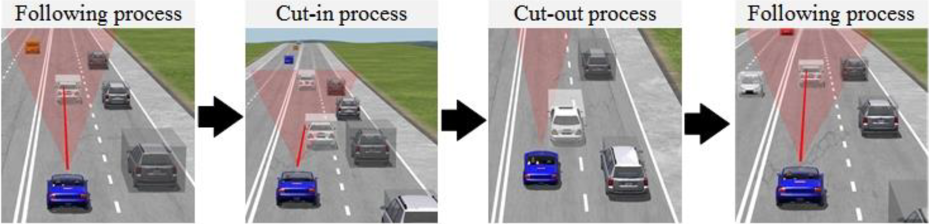
The simulation conditions for a comparative test.

One difference from the traditional decision-making method is that the proposed method based on the reinforcement Q-learning algorithm uses a Q-table to update and transfer the state. For example, Figure 18 shows the action selection mechanism for an acceleration process and deceleration process.

Figure 18.

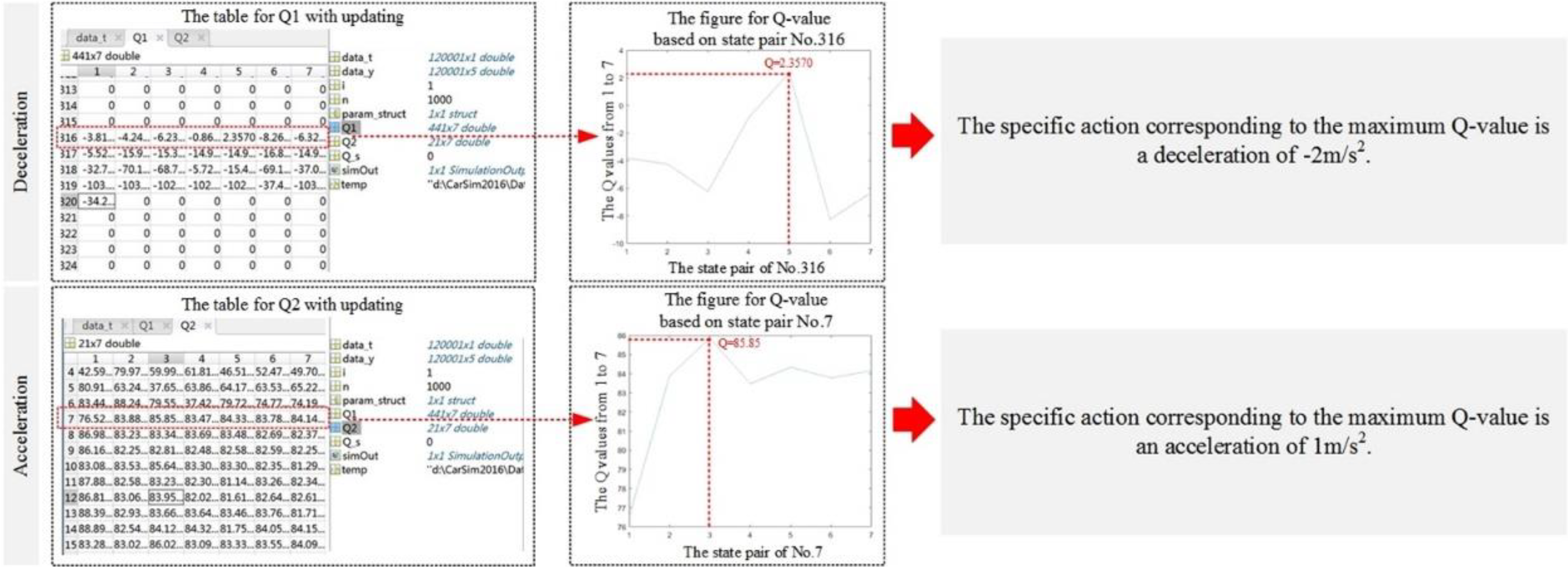
The action selection mechanism for an acceleration process and deceleration process.

Figure 19 shows the comparison of acceleration, it is clear that the curve of the traditional method is continuous and the proposed method is discontinuous.

Figure 19.

The comparative acceleration results of the two methods.

Results analysis

The simulation results for the constant speed tests indicate that the proposed method has feasibility and effectiveness in the cruising process. The simulation results for the variable speed tests indicate that the proposed method has adaptive capacity for random driving conditions.

Moreover, by the comparison of different decision-making methods, it is obvious that the traditional acceleration curve has mutations during cut-in and cut-out processes. However, the proposed method eliminates mutations through its learning mechanism and interaction ability, and this finding also improves the comfort and adaptive capability of the vehicle.

Conclusions and future work

In this article, we propose an independent decision-making method based on a reinforcement Q-learning algorithm for vehicle longitudinal automatic driving. In addition, the main contributions are as follows: (1) A traditional rule-based decision-making method is replaced by an independent decision-making method. (2) An MDP model is established by analysis of car-following. (3) Driving simulator experiments and driving risk principles are provided for the design of the algorithm. (4) A reinforcement Q-learning algorithm is developed mainly based on the design of the reward function and the update function. (5) The feasibility is verified through random simulation tests. (6) Improvement is made by comparative analysis with the traditional method.

However, there are still some limitations of the proposed model. First, this model is more suitable for traditional passenger vehicles because of its dynamic characteristics. Second, the reward functions lack detailed classification among different following conditions. Finally, the stability of the model is not verified.

In future work, the reward functions can be improved by considering comfort. The stability of the model could be verified by a real vehicle test.

Footnotes

Acknowledgements

The authors gratefully acknowledge Zhenhai Gao, Hongwei Xiao, and Lei He of Jilin University for their helpful discussion.

Declaration of conflicting interests

The authors declared no potential conflicts of interest with respect to the research, authorship, and/or publication of this article.

Funding

The authors disclosed receipt of the following financial support for the research, authorship, and/or publication of this article: This work was supported by National Key Research and Development Program of China (grant no. 2017YFB0102600).

ORCID iD

Hongwei Xiao

References

Weilong

. Research on behavioral decision making for intelligent vehicles in dynamic urban environments. Beijing: Beijing Institute of Technology, 2016.

Gao

Cheng

Wang

. Object classification using CNN-based fusion of vision and LIDAR in autonomous vehicle environment. IEEE Trans Ind Inform 2018; 14: 4224–4231.

Xie

Gao

Qian

. Vehicle trajectory prediction by integrating physics- and maneuver-based approaches using interactive multiple models. IEEE Trans Ind Electron 2018; 65: 5999–6008.

Jun

. Research on multi-objective perception-decision-control algorithm for adaptive cruise control systems. Changchun: Jilin University, 2015.

Vanderhaegen

Zieba

. Reinforced learning systems based on merged and cumulative knowledge to predict human actions. Inf Sci 2014; 276: 146–159.

Desjardins

Chaib-Draa

. Cooperative adaptive cruise control: a reinforcement learning approach. IEEE Trans Intell Transp Syst 2011; 12: 1248–1260.

Rui

. Reinforcement learning-based intelligent decision-making methods for unmanned vehicles. Changsha: National University of Defense Technology, 2013.

Chunming

. Research on autonomous driving on highway roads based on reinforcement learning and vehicle dynamics. Changsha: National University of Defense Technology, 2014.

Chong

Abbas

Flintsch

. A rule-based neural network approach to model driver naturalistic behavior in traffic. Transp Res Part C Emerg Technol 2013; 32: 207–223.

10.

Gao

. A hardware platform framework for an intelligent vehicle based on a driving brain. Engineering 2018; 4: 464–470.

11.

Yan

Study on adaptive cruise control algorithms imitating car-following behaviors of drivers. PhD Thesis, Jilin University, Changchun, 2016.

12.

Chen

Zhai

. A learning model for personalized adaptive cruise control. In: 2017 IEEE intelligent vehicles symposium (IV), Los Angeles, CA, USA, 11–14 June 2017, pp. 379–384. IEEE. DOI: 10.1109/IVS.2017.7995748.

13.

Hester

Lopes

Stone

. Learning exploration strategies in model-based reinforcement learning. In: The 12th international conference in autonomous agents and multiagent systems (AAMAS) (eds Ito, Jonker, Gini, and Shehory), St Paul, MN, USA, 6-10 May 2013, pp. 1069–1076. IEEE.

14.

Maozu

Yang

Tiyun

. Comparative study of the main reinforcement learning algorithms. Int J Comput Eng Appl 2001; 21: 16–18.

15.

Shi

. Modeling driver’s car-following behavior based on hidden Markov model and model predictive control: a cyber-physical system approach. In: 2017 11th Asian control conference (ASCC), Gold Coast, QLD, Australia, 17–20 December 2017, pp. 114–119. IEEE. DOI: 10.1109/ASCC.2017.8287152.

16.

Miao

. Study and experiment of reinforcement learning algorithm. Xi’an: Xidian University, 2014.

17.

Gao

Sun

. A multi-mode control strategy for EV based on typical situation. SAE Technical Paper 2017-01-0438, 2017.

18.

Liang

. A driver behavior decision model based on multi-agent systems. Chongqing: Southwest University, 2010.

19.

Solomon

. Accidents on main rural highways related to speed, drivers and vehicle. Washington: Bureau of Public Road, 1964.

20.

Rigolli

Brady

. Towards a behavioural traffic monitoring system. In: Proceedings of the fourth international joint conference on autonomous agents and multiagent systems (eds, Dignum

Dignum

Koenig

), The Netherlands, 25–29 July 2005, pp. 449–454. New York: ACM Press.