Stable emergent formations for a swarm of autonomous car-like vehicles

Abstract

A biological swarm is an ideal multi-agent system that collectively self-organizes into bounded, if not stable, formations. A mathematical model, developed appropriately from some principle of swarming, should enable one, therefore, to study formation strategies for multiple autonomous robots. In this article, based on the hypothesis that swarming is an interplay between long-range attraction and short-range repulsion between the individuals in the swarm, a planar individual-based or Lagrangian swarm model is constructed using the Direct Method of Lyapunov. While attraction ensures the swarm is cohesive, meaning that the individuals in the swarm remain close to each other at all times, repulsion ensures that the swarm is well-spaced, meaning that no two individuals in the swarm occupy the same space at the same time. Via a novel Lyapunov-like function with attractive and repulsive components, the article establishes the global existence, uniqueness, and boundedness of solutions about the centroid. This paves the way to prove that the swarm model, governed by a system of first-order ordinary differential equations (ODEs), is cohesive and well-spaced. The article goes on to show that the artificial swarm can collectively self-organize into two stable formations: (i) a constant arrangement about the centroid when the system has equilibrium points, and (ii) a highly parallel formation when the system does not have equilibrium points. Computer simulations not only illustrate these but also reveal other emergent patterns such as swirling structures and random-like walks. As an application, we tailor the model accordingly and propose new autonomous steering laws giving rise to pattern-forming for multiple nonholonomic car-like vehicles.

Introduction

An interesting research domain in robotics is formation control. This involves the design of controllers for multiple mobile agents such that the agents move in some bounded, if not stable, formation without colliding with each other or with obstacles. ¹ Recent applications are seen in the control of pattern formation of fleets of autonomous car-like vehicles or swarms of unmanned aerial vehicles for tasks such as aiding traffic management of automated highways, environmental monitoring, search-and-rescue in hazardous environments, and area coverage and reconnaissance. ^{2 –4}

An exciting development in this area of research is the use of swarm principles to design the controllers. Animal swarming is considered an instance of collective self-organization, which is defined in the study by Camazine et al. ⁵ as “a broad range of pattern-formation processes in both physical and biological systems, with the pattern being an emergent property of the system, rather than a property imposed on the system by an external ordering influence.” It has been hypothesized that animal swarming is an interplay between long-range attraction and short-range repulsion between the individuals in the swarm; attraction ensures a cohesive swarm while repulsion ensures a well-spaced swarm. ^{6 –8} An artificial swarm model developed appropriately from such a notion should thus exhibit emergent patterns such as (i) constant arrangements about a stationary centroid as seen, for example, in myxobacterial fruiting body formation, ^9,10 (ii) parallel formations seen in columns of ants, ^11,12 (iii) circular or oscillatory formations such as milling structures in schools of fish, ¹³ and (iv) random walks such as the Lévy flight which describes a seemingly random but bounded pattern of foraging and animal hunting. ¹⁴ An exhaustive list of emergent patterns is provided in the study by Camazine et al. ⁵ An interesting new direction of enquiry in formation control deals with how to control an artificial swarm to settle into a desired pattern. ¹⁵

The efforts of researchers over the last three decades to understand swarming have resulted in two different approaches to modeling; the Eulerian and the Lagrangian approaches. ¹⁶ In the Eulerian approach, the swarm is considered a continuum described by its density in one-, two- or three-dimensional space. The time evolution of swarm density is described by partial differential equations. In the Lagrangian approach, the state (position, instantaneous velocity and instantaneous acceleration) of each individual and its relationship with other individuals in the swarm is studied; it is an individual-based approach, in which the velocity and acceleration can be influenced by spatial coordinates of the individual. The time evolution of the state is described by ordinary or stochastic differential equations. A review of different approaches can be found in the study by Carrillo et al. ¹⁷ A recent analysis of cohesiveness in a Lagrangian-type model incorporating collision avoidance is given in the study by Li. ¹⁸

An alternative approach to understanding coherent swarm structures can be traced to the work of physicists who consider individuals in a swarm as self-propelling particles governed by discrete equations. ¹⁹ These models of discrete swarm structure use iterative methods which provide recursion formulas that update the position, velocity, and orientation of an individual with respect to other individuals. Extensive simulations are required to validate the models, the simplest of which merely assume that individuals move at a constant speed, and, at each time step, each one travels in the average direction of motion of those within a local neighborhood. A similar approach adopted by computer scientists is called the particle swarm optimization, wherein the velocity and position of a point mass is governed by a computer algorithm rather than differential or discrete equations. A recent survey of methods can be found in. ²⁰

The swarm model proposed in this study is individual-based or Lagrangian. Adopting the hypothesis that swarming is an interplay between long-range attraction and short-range repulsion between the individuals in the swarm, we consider spacing between individuals, each of which moves with the velocity of the swarm centroid, of primary importance. While attraction ensures cohesiveness, meaning that the individuals in the swarm remain close to each other at all times, repulsion ensures it is well-spaced, meaning that no two individuals in the swarm occupy the same space at the same time. To our knowledge, the cohesiveness and well-spaced notions are being treated for the first in a rigorous manner in this article. The method utilized is the Direct Method of Lyapunov via which a Lyapunov-like function with attractive and repulsive components is constructed. The function enables us to establish the existence, uniqueness, and boundedness of solutions about the centroid. This paves the way to prove that the swarm model, governed by a system of first-order ordinary differential equations (ODEs), is cohesive and well-spaced. We go on to show that the model can collectively self-organize into two stable formations: (i) a constant arrangement about the centroid when the system has equilibrium points, and (ii) a highly parallel formation when the system has no equilibrium points. Computer simulations not only illustrate these but also reveal other emergent patterns such as swirling structures and random-like walks. The results in this article are new or are a refinement of the author’s work thus far in this area. ^21,22

We begin by developing the model in the “A two-dimensional Lagrangian swarm model” section, deriving the velocity controller of each individual via a Lyapunov-like function in the “Velocity controllers” section and discussing the properties of the function in the “Roles of the parameters in the Lyapunov-like function” section. Before we provide the main result of this article in the “A well-placed and cohesive system” section, which is on boundedness, we give several illuminating and insightful examples of the model dynamics in the “Examples of system behavior” section. We then proceed to look at situations when equilibrium points can exist (“Equilibrium points of system (4)” section) and when they cannot, in which case a pattern emerges, namely the parallel formation (“Parallel formation in the absence of equilibrium” section). The results are applied accordingly to a swarm of autonomous nonholonomic planar vehicles (“Application to planar mobile car-like vehicles” section).

A two-dimensional Lagrangian swarm model

We begin the construction of our swarm model by adopting two terms from Mogilner et al. ¹⁶ as working definitions of a swarm. The rigorous definitions of the terms are given at the end of this section.

A system is well-spaced if the system represents a group which does not collapse into a tight cluster.

A system is cohesive if the system represents a group in which the distances between individuals in the group are bounded from above.

A swarm is a well-spaced and cohesive system that represents a group or aggregate of individuals.

Consider a swarm of $n\in \mathbb{N}$ individuals. Following previous work such as those in Mogilner et al. ¹⁶ and Gazi and Passino, ⁶ we consider the individuals as point masses. At time $t\ge 0$ , let $(x_i(t),y_i(t))$ , $i=1,2,\dots ,n$ , be the planar position of the ith individual, which we shall define as a point mass residing in a disk of radius $r_V>0$ ,

$A_i:=\{(z_1,z_2)\in {ℝ}^2:(z_1-x_i{)}^2+{(z_2-y_i)}^2\le r_V^2\}$

1

The disk is described in Mogilner et al. ¹⁶ as a bin, and in Gazi and Passino ⁶ as a private or safety area of each individual. We shall use the former term, with the bin size being the radius r_V of the disk. As noted in Mogilner et al., ¹⁶ the members of a cohesive swarm tend to stay together and avoid dispersing. In a well-spaced swarm, some minimal bin size exists such that each bin contains at most one individual. Moreover, the size of such a bin is independent of the number of individuals in the group.

Let us define the centroid of the swarm as

$(x_C,y_C):=\left(\frac{1}{n}{\displaystyle \sum _{k=1}^n}{x}_k,\frac{1}{n}{\displaystyle \sum _{k=1}^n}{y}_k\right)$

2

At time $t\ge 0$ , let $(v_i(t),w_i(t)):=({x^{\prime }}_i(t),{y^{\prime }}_i(t))$ be the instantaneous velocity of the ith point mass. Using the above notations, we have thus a system of first-order ODEs for the ith individual, assuming the initial condition at $t=t_0\ge 0$

${x^{\prime }}_i(t)=v_i(t),\hspace{0.17em}\hspace{0.17em}{y^{\prime }}_i(t)=w_i(t),\hspace{0.17em}\hspace{0.17em}{x}_{i0}:=x_i(t_0),\hspace{0.17em}\hspace{0.17em}{y}_{i0}:=y_i(t_0)$

3

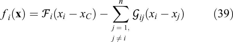
Suppressing t, we let $x_i:=(x_i,y_i)\in {ℝ}^2$ and $x:=(x_1,\dots ,x_n)\in {ℝ}^{2n}$ be our state vectors. Also, let $x_0=(x_{10},y_{10},\dots ,x_{n0},y_{n0}):=x(t_0)\in {ℝ}^{2n}$ . If the instantaneous velocity $(v_i,w_i)$ has a state feedback law of the form $(v_i(t),w_i(t))=(-{\mu }_i{f}_i(x(t)),-{\phi }_i{g}_i(x(t)))$ , $i\in 1,\dots ,n$ , for some constants ${\mu }_i,{\phi }_i>0$ and some continuous functions $f_i(x(t))$ and $g_i(x(t))$ , to be constructed appropriately later, and if we define $g_i(x):=(-{\mu }_i{f}_i(x),-{\phi }_i{g}_i(x))\in {ℝ}^2$ and $G(x):=(g_1(x),\dots ,g_n(x))\in {ℝ}^{2n}$ , then our swarm of n individuals is

$\stackrel{•}{x}=G(x),\hspace{0.17em}\hspace{0.17em}{x}_0=x(t_0)$

4

If the system has an equilibrium point, we shall denote it by

$x_e:=(x_{1e},x_{2e},\dots ,x_{ne}):=(x_{1e},y_{1e},x_{2e},y_{2e},\dots ,x_{ne},y_{ne})\in {ℝ}^{2n}$

We end this section by rigorously defining a well-spaced and cohesive system. Let $x_C:=\left(x_C,y_C,\dots ,x_C,y_C\right)\in {ℝ}^{2n}$ ,

$\parallel x-x_C\parallel :=\sqrt{{\displaystyle \sum _{i=1}^n}\left[{\left(x_i-x_C\right)}^2+{\left(y_i-y_C\right)}^2\right]},$

and $d_{iC}:=\sqrt{{\left[x_i-x_C\right]}^2+{\left[y_i-y_C\right]}^2},$ for $i=1,\dots ,n$ .

Definition 2.1

System (4) is well-spaced if the solution of system (4) exists for all $t\ge 0$ and

$d_{ij}(t):=\parallel x_i(t)-x_j(t)\parallel =\sqrt{{\left[x_i(t)-x_j(t)\right]}^2+{\left[y_i(t)-y_j(t)\right]}^2}>2r_V$

for all $i,j=1,\dots ,n$ , $i\ne j$ , and $t\ge 0$ .

Lemma 2.2

If system (4) is well-spaced, then $r_V<\parallel x(t)-x_C(t)\parallel$ for all $t\ge 0$ .

Proof

If the outcome of Lemma 2.2 is false, then there must be a time $t^{\prime }\ge 0$ such that $\parallel x(t^{\prime })-x_C(t^{\prime })\parallel \le r_V$ . Then for every $i=1,\dots ,n$ , we have that $d_{iC}(t^{\prime })\le \parallel x(t^{\prime })-x_C(t^{\prime })\parallel \le r_V$ . Consequently, for some two $i,j$ , $i\ne j$ , $i,j=1,\dots ,n$ , it is possible that $d_{ij}(t^{\prime })\le d_{iC}(t^{\prime })+d_{iC}(t^{\prime })\le 2r_V$ , which contradicts Definition 2.1.

Note if $n=1$ , then $\parallel x-x_C\parallel =0$ . Hence, the idea of a well-spaced swarm makes sense only if $n\ge 2$ .

For cohesiveness, we adopt the following rigorous definition by Lemmon and Sun ²³ :

Definition 2.3

System 4 is cohesive if there exist real constants $\overline{K},\underset{\_}{K}>0$ such that ${{\displaystyle \text{lim}\hspace{0.17em}\text{sup}}}_{t\to \infty }\parallel x(t)-x_C(t)\parallel \le \overline{K}$ and ${{\displaystyle \text{lim}\hspace{0.17em}\text{inf}}}_{t\to \infty }\parallel x(t)-x_C(t)\parallel \ge \underset{\_}{K}$ .

Obviously the two limits exist if $\parallel x(t)-x_C(t)\parallel <\infty$ for all $t\ge 0$ .

Velocity controllers

Our control objective is to construct the functions $f_i(x(t))$ and $g_i(x(t))$ , and hence the instantaneous velocity $(v_i(t),w_i(t))$ , $t\ge 0$ , for every individual $i=1,\dots ,n$ , via a Lyapunov-like function that should establish the boundedness and therefore the cohesiveness of system (4).

Attraction to the centroid

We can ensure that individuals are attracted to each other and also form a cohesive group by having a measure of the distance from the ith individual to the swarm centroid. This is the concept behind flock-centering or cohesion, which is one of the well-known three heuristic flocking rules of Reynolds’ applied to virtual agents he called boids ²⁴ :

Separation: Each boid must steer to avoid colliding with local flock-mates;

Alignment: Each boid must steer toward the average heading of local flock-mates; and

Cohesion: Each boid must steer to move toward the average position (center of mass or centroid) of local flock-mates.

Flock-centering minimizes the exposure of a member of a flock to the flock’s exterior by having the member move toward the perceived center of the flock. It is therefore a form of attraction between individuals. Centering necessitates a measure of the distance from the ith individual to the swarm centroid. For this purpose, we consider the function

$R_i(x):=\frac{1}{2}\left[{\left(x_i-x_C\right)}^2+{\left(y_i-y_C\right)}^2\right]+{\epsilon }_i^2,\hspace{0.17em}\hspace{0.17em}i=1,\dots ,n$

5

where ${\epsilon }_i>0$ are sufficiently small constants. As we shall see later, the role of the constants is to ensure that system (4) has a global solution $x(t)$ which is defined for all time $t\ge 0$ . We remind ourselves of the importance of the existence of global solutions for system (4) to be well-spaced (see Definition 2.1).

Interindividual collision avoidance

The short-range repulsion between individuals necessitates utilizing a measurement of the distance between the i th and the j th individuals, $j\ne i$ , $i,j=1,\dots ,n$ . For this purpose, we consider the function

$Q_{ij}(x):=\frac{1}{2}\left[{\left(x_i-x_j\right)}^2+{\left(y_i-y_j\right)}^2-{(2r_V)}^2\right]$

6

A Lyapunov-like function

To obtain the appropriate instantaneous velocity of the individuals, we construct a Lyapunov-like function. Accordingly, let there be constants ${\gamma }_i>0$ and ${\beta }_{ij}>0$ , and define, for $i,j=1,\dots ,n$

$L_i(x):={\gamma }_i{R}_i(x)+{\displaystyle \sum _{\begin{array}{l}j=1,\\ j\ne i\end{array}}^n\frac{{\beta }_{ij}{R}_i(x)}{Q_{ij}(x)}}$

Consider as a tentative Lyapunov-like function for system (4)

$L(x):={\displaystyle \sum _{i=1}^n}{L}_i(x_i)$

7

It is positive over the domain

$D(L):=\left\{x\in {ℝ}^{2n}:Q_{ij}(x)>0\hspace{0.17em}\forall \hspace{0.17em}i,j=1,\dots ,n,i\ne j\right\}$

8

The time-derivative of L along every solution of system (4) is

${\stackrel{•}{L}}_{(4)}(x)={\displaystyle \sum _{i=1}^n}\left({\gamma }_i{\stackrel{•}{R}}_i(x)+{\displaystyle \sum _{\begin{array}{l}j=1,\\ j\ne i\end{array}}^n\frac{{\beta }_{ij}}{Q_{ij}(x)}{\stackrel{•}{R}}_i(x)-{\displaystyle \sum _{\begin{array}{l}j=1,\\ j\ne i\end{array}}^n\frac{{\beta }_{ij}{R}_i(x)}{Q_{ij}^2(x)}{\stackrel{•}{Q}}_{ij}(x)}}\right)$

where

${\displaystyle \sum _{i=1}^n}{\stackrel{•}{R}}_i(x)={\displaystyle \sum _{i=1}^n}\left[\left(x_i-\frac{1}{n}{\displaystyle \sum _{k=1}^n}{x}_k\right)-\frac{1}{n}{\displaystyle \sum _{m=1}^n}\left(x_m-\frac{1}{n}{\displaystyle \sum _{k=1}^n}{x}_k\right)\right]{x^{\prime }}_i+{\displaystyle \sum _{i=1}^n}\left[\left(y_i-\frac{1}{n}{\displaystyle \sum _{k=1}^n}{y}_k\right)-\frac{1}{n}{\displaystyle \sum _{m=1}^n}\left(y_m-\frac{1}{n}{\displaystyle \sum _{k=1}^n}{y}_k\right)\right]{y^{\prime }}_i$

Noting that $\frac{1}{n}{\displaystyle \sum _{m=1}^n\left(u_m-\frac{1}{n}{\displaystyle \sum _{k=1}^n{u}_k}\right)=0}$ for any $u_i\in ℝ$ , $i=1,2,\dots ,n$ , we simplify the expression to

${\displaystyle \sum _{i=1}^n}{\stackrel{•}{R}}_i(x)={\displaystyle \sum _{i=1}^n}\left[\left(x_i-\frac{1}{n}{\displaystyle \sum _{k=1}^n}{x}_k\right)x_i\text{'}+\left(y_i-\frac{1}{n}{\displaystyle \sum _{k=1}^n}{y}_k\right){y^{\prime }}_i\right]$

Also, we can show that

${\displaystyle \sum _{i=1}^n}{\displaystyle \sum _{\begin{array}{l}j=1,\\ j\ne i\end{array}}^n{\stackrel{•}{Q}}_{ij}(x)=2}{\displaystyle \sum _{i=1}^n}{\displaystyle \sum _{\begin{array}{l}j=1,\\ j\ne i\end{array}}^n(x_i-x_j){x^{\prime }}_i+2}{\displaystyle \sum _{i=1}^n}{\displaystyle \sum _{\begin{array}{l}j=1,\\ j\ne i\end{array}}^n(y_i-y_j){y^{\prime }}_i}$

Collecting terms with $x_i\text{'}$ and $y_i\text{'}$ , and substituting ${x^{\prime }}_i={\stackrel{•}{x}}_i=v_i$ and ${y^{\prime }}_i={\stackrel{•}{y}}_i=w_i$ from system (3), we have, along a trajectory of system (4) (on suppressing $x$ )

${\stackrel{•}{L}}_{(4)}={\displaystyle \sum _{i=1}^n}\left\{\left({\gamma }_i+{\displaystyle \sum _{\begin{array}{l}j=1,\\ j\ne i\end{array}}^n\frac{{\beta }_{ij}}{Q_{ij}}}\right)\left(x_i-\frac{1}{n}{\displaystyle \sum _{k=1}^n}{x}_k\right)-2{\displaystyle \sum _{\begin{array}{l}j=1,\\ j\ne i\end{array}}^n\frac{{\beta }_{ij}{R}_i}{Q_{ij}^2}(x_i-x_j)}\right\}{\stackrel{•}{x}}_i+{\displaystyle \sum _{i=1}^n}\left\{\left({\gamma }_i+{\displaystyle \sum _{\begin{array}{l}j=1,\\ j\ne i\end{array}}^n\frac{{\beta }_{ij}}{Q_{ij}}}\right)\left(y_i-\frac{1}{n}{\displaystyle \sum _{k=1}^n}{y}_k\right)-2{\displaystyle \sum _{\begin{array}{l}j=1,\\ j\ne i\end{array}}^n\frac{{\beta }_{ij}{R}_i}{Q_{ij}^2}}(y_i-y_j)\right\}{{\displaystyle \stackrel{•}{y}}}_i$

Let

$f_i:=f_i(x)=\left({\gamma }_i+{\displaystyle \sum _{\begin{array}{l}j=1,\\ j\ne i\end{array}}^n\frac{{\beta }_{ij}}{Q_{ij}}}\right)\left(x_i-\frac{1}{n}{\displaystyle \sum _{k=1}^n}{x}_k\right)-2{\displaystyle \sum _{\begin{array}{l}j=1,\\ j\ne i\end{array}}^n\frac{{\beta }_{ij}{R}_i}{Q_{ij}^2}(x_i-x_j)}$

9

and

$g_i:=g_i(x)=\left({\gamma }_i+{\displaystyle \sum _{\begin{array}{l}j=1,\\ j\ne i\end{array}}^n\frac{{\beta }_{ij}}{Q_{ij}}}\right)\left(y_i-\frac{1}{n}{\displaystyle \sum _{k=1}^n}{y}_k\right)-2{\displaystyle \sum _{\begin{array}{l}j=1,\\ j\ne i\end{array}}^n\frac{{\beta }_{ij}{R}_i}{Q_{ij}^2}(y_i-y_j)}$

10

Thus

${\stackrel{•}{L}}_{(4)}={\displaystyle \sum _{i=1}^n}(f_i{x^{\prime }}_i+g_i{y^{\prime }}_i)={\displaystyle \sum _{i=1}^n}(f_i{v}_i+g_i{w}_i)$

Let there be numbers ${\mu }_i>0$ and ${\phi }_i>0$ such that

$v_i:=-{\mu }_i{f}_i\hspace{0.17em}\hspace{0.17em}\text{and}\hspace{0.17em}\hspace{0.17em}{w}_i:=-{\phi }_i{g}_i$

11

Then

${\stackrel{•}{L}}_{(4)}(x)=-{\displaystyle \sum _{i=1}^n}\left[{\mu }_i{f}_i^2(x)+{\phi }_i{g}_i^2(x)\right]\le 0$

for all $x\in D(L)$ .

We have thus obtained a simple Lagrangian swarm model in the form of system (4) with components (3), where the velocity components are given in (11).

Roles of the parameters in the Lyapunov-like function

As we shall see in later sections, the parameters in the Lyapunov-like function play the major role in inducing a particular stable pattern. In this section, we provide an overview of the roles of the parameters.

Consider again our Lyapunov-like function (7). At large distances between the i th and the j th individuals, the ratio

${\displaystyle \sum _{i=1}^n}{\displaystyle \sum _{\begin{array}{l}j=1,\\ j\ne i\end{array}}^n\frac{{\beta }_{ij}{R}_i(x)}{Q_{ij}(x)}}$

12

is negligible, and the term ${\displaystyle \sum _{i=1}^n{\gamma }_i{R}_i(x)}$ dominates and acts as the attraction function; each individual is attracted to the centroid, and therefore system (4), as we shall show rigorously in the “A well-placed and cohesive system” section, maintains cohesiveness at all times. Thus, the parameter ${\gamma }_i>0$ can be considered as a measurement of the strength of attraction between an individual i and the swarm centroid $(x_C,y_C)$ . The smaller the parameter is, the weaker the cohesion of the swarm is. Hence, ${\gamma }_i$ can be called a cohesion parameter.

Consider now the situation where any two individuals i and j approach each other. In this case, $Q_{ij}$ decreases and ratio (12) increases, with ${\beta }_{ij}>0$ acting as a coupling parameter that is a measurement of the strength of interaction between the individuals. In this way, ratio (12) acts as an interindividual collision avoidance function, because it can be allowed to increase in value (corresponding to avoidance) as individuals approach each other. However, as we show rigorously in the “A well-placed and cohesive system” section, collision avoidance occurs without the danger of the individuals getting too close to each other, or the swarm collapsing on itself; simply put, $Q_{ij}=0$ is not possible in $D(L)$ . We have therefore met the short-range repulsion requirement in an individual-based model. Note that the increase in the ratio (12) does not translate to an increase in $L\equiv L(t)$ , simply because L is nonincreasing in t and any increase in the ratio gives a smaller or the same value of L at time t compared to all previous values of L.

We have used two other parameters, ${\mu }_i>0$ and ${\phi }_i>0$ in system (4). Because the parameters are a measure of the rate of decrease of $L\equiv L(t)$ at time $t\ge 0$ , we name them convergence parameters. The larger the convergence parameters, the quicker the movements of the individuals toward and about the centroid.

In summary, the cohesion parameters ( ${\gamma }_i>0$ ), the coupling parameters ( ${\beta }_{ij}>0$ ), and the convergence parameters ( ${\mu }_i,{\phi }_i>0$ ) make up the control parameters of the system.

Examples of system behavior

Before we consider the existence, uniqueness, and boundedness of solutions of system (4) in the next section, we look at some interesting dynamics of the system. These illustrations will deepen our intuitive insight into the behavior of the solutions.

Example 5.1 (constant arrangement about the centroid)

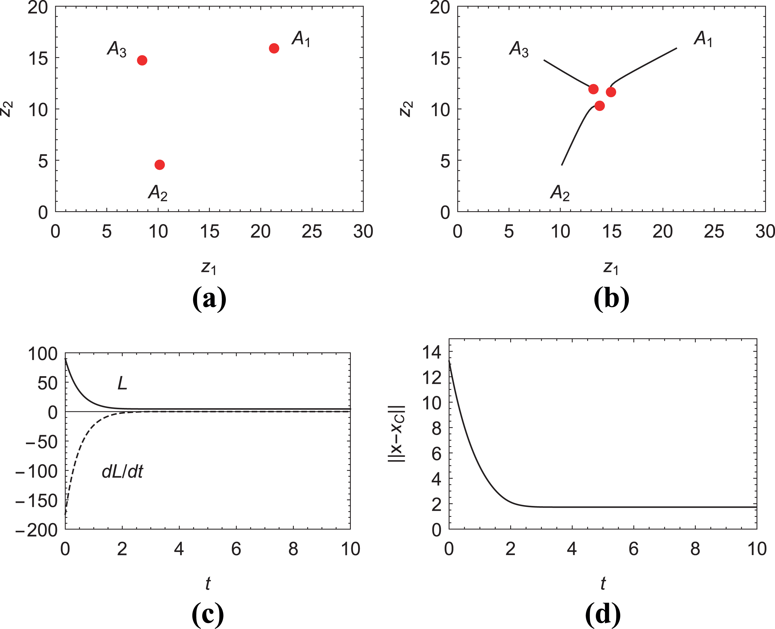
In this example, we consider a swarm of three individuals, each with bin size $r_V=1/2$ . With ${\epsilon }_i{=10}^{-6}$ and the control parameters set at ${\mu }_i={\phi }_i={\gamma }_i={\beta }_{ij}=1$ , $i,j=1,2,3$ , it is seen in Figure 1 that system (4) has an equilibrium point.

Figure 1.

The initial positions of the three point masses A₁, A₂, and A₃ are shown in diagram (a). They are $x_1(0)=(21.3,15.9)$ , $x_2(0)=(10.2,4.6)$ , and $x_3(0)=(8.4,14.7)$ , respectively. Diagram (b) shows the positions where A₁, A₂, and A₃ ceased motion. They are $x_{1e}=(14.9,11.6)$ , $x_{2e}=(13.8,10.3)$ , and $x_{3e}=(13.2,11.9)$ , respectively. Thus, $x_e=(x_{1e},x_{2e}\mathrm{.}{x}_{2e})$ . Diagram (c) shows the monotonic Lyapunov-like function with $4.5\le L\le 89.8$ and $-174.6\le \text{d}L/\text{d}t\le 0$ for all $t\ge 0$ . Diagram (d) shows that the solution $x$ are bounded about the centroid $x_C$ .

Example 5.2 (parallel formation)

In this example, with $n=10$ individuals, each with bin size $r_V=1/2$ , the swarm eventually moves in a straight line, with the each individual heading in the same direction and angle. The individuals A₄, A₇, A₆, and A₅ follow the centroid’s trajectory (central thick line in Figure 2), with the emergent leader being A₄. The others follow paths parallel to it, with A₁, A₃, A₈, and $A_{10}$ in the outer lanes, and A₂ and A₉ in the inner lanes.

Figure 2.

With the given initial positions shown in (a), and the choices ${\epsilon }_i{=10}^{-6}$ and ${\mu }_i={\varphi }_i={\gamma }_i={\beta }_{ij}=1$ , $i,j=1,\dots \mathrm{,8}$ , the point masses eventually move in a parallel formation, as shown in diagram (b) by $t=50$ units of time. In diagram (c), the monotonic Lyapunov-like function is shown, with $109.28\le L\le 657.04$ and $-1058.14\le \text{d}L/\text{d}t\le -0.91$ which implies that the system of point masses does not cease motion and eventually cruises with a constant speed. Diagram (d) shows that the solution $x$ of system (4) is bounded about the centroid.

Example 5.3 (swirling structure)

In this example, with $n=12$ , the point masses, each with bin size $r_V=1/2$ , seem to wander randomly before settling down to a swirling pattern. The cohesion parameters, γ_i, are set at 1, the coupling parameters, ${\beta }_{ij}$ , are randomized between and including 1 and 30, and the convergence parameters, μ_i and φ_i, at set at 1. The constants ε_i are chosen to be ${10}^{-6}$ . Figure 3 shows the positions of the point masses at $t=387$ units of time, the monotone nature of the Lyapunov-like function, and the boundedness of solution $x$ with respect to the centroid $x_C$ .

Figure 3.

The dashed line in diagram (a) plots the trajectory of the centroid, which clearly shows an emergent swirling structure with an empty core. In diagram (b), we have that $1703.03\le L\le 11,074.60$ and $-45,014.90\le \text{d}L/\text{d}t\le -42.99$ which implies that the system of point masses does not cease motion. Diagram (c) shows that around the centroid, the movements are erratic but bounded before settling down.

Example 5.4 (random-like walks)

A random walk is a random process consisting of a sequence of discrete steps of fixed length. ²⁵ In this example, with $n=30$ , the point masses, each with bin size $r_V=10$ , display random-like walks. The cohesion parameters are ${\gamma }_i=1$ , the coupling parameters, ${\beta }_{ij}$ , are randomized between and including 100 and 600, the convergence parameters μ_i and φ_i, are set at 5, and the constants ε_i are chosen to be ${10}^{-6}$ . In Figure 4, the grayish areas are trajectories of each individual, whereas the black trajectory is the trace of the centroid, given over the time period $t\in [0,3000]$ .

Figure 4.

The simulation shows a cohesive group with individuals hovering excitedly about the centroid in a random fashion. As they change positions, the centroid traces out a series of straight segments interrupted by tight turns. As in previous examples, the Lyapunov-like function is monotonic, and the solution is bounded about the centroid. (a) A random-like walk and (b) a zoomed-in centroid path at t = 500.

A well-spaced and cohesive system

The examples in the previous section provide helpful intuitive insights into the behavior of system (4). They seem to suggest that the solutions are bounded about the centroid. In this section, we will show that, indeed, it is the case. We begin by showing that system (4) is well-spaced, which, according to Definition 2.1, means that the solution $x(t)$ of system (4) exists and is unique for all time $t\ge 0$ in the domain $D(L)$ .

A well-spaced system

Looking at the right-hand side of equations (9) and (10), we see that the functions that appear in the denominator are $Q_{ij}$ , $i,j\in \mathbb{N}$ , $i\ne j$ . Hence, we can easily conclude that $G\in C[D(L),{ℝ}^{2n}]$ , which implies that at least on some time interval $[t_0,\alpha ]$ , $\alpha >0$ , the solution $x(t)$ of system (4) exists and is in $D(L)$ . Indeed, since the functions $Q_{ij}$ appear in the denominator in (9) and (10), they will also appear in the denominator in higher-order partial derivatives, with each derivative continuous on $D(L)$ . This means that $G$ is locally Lipschitz on $D(L)$ , that is, $G\in C^1[D(L),{ℝ}^{2n}]$ . This implies the solution $x(t)$ of system (4) exists and is unique in $D(L)$ on the time interval $[t_0,\alpha ]$ .

We shall next attempt to show that $x(t)$ exists and is unique for all time $t\ge t_0\ge 0$ in $D(L)$ .

We begin by observing that since the time-derivative of L along the solution of (4) is nonpositive, we have

$L(x(t))\le L_0:=L(x_0),\hspace{0.17em}\hspace{0.17em}t\in [t_0,\alpha ]$

13

From the form of L in (7), equation (13) implies that for every $i\ne j$ , $i,j=1,\dots ,n$

${\gamma }_i{R}_i(x(t))\le L_0\hspace{0.17em}\hspace{0.17em}\text{and}\hspace{0.17em}\hspace{0.17em}{\beta }_{ij}\frac{R_i(x(t))}{Q_{ij}(x(t))}\le L_0,\hspace{0.17em}t\in [t_0,\alpha ]$

14

Let $r_0:=\text{max}\{L_0/{\gamma }_i,\hspace{0.17em}i=1,\dots ,n\}$ and $q_0:=\text{max}\{L_0/{\beta }_{ij},i\ne j,\hspace{0.17em}i,j=1,\dots ,n\}$ . Then from (14), we get

$R_i(x(t))\le r_0\hspace{0.17em}\hspace{0.17em}\text{and}\hspace{0.17em}\hspace{0.17em}\frac{R_i(x(t))}{Q_{ij}(x(t))}\le q_0,\hspace{0.17em}\hspace{0.17em}t\in [t_0,\alpha ]$

15

Given the form of $R_i(x(t))$ in (5), the second inequality in (15) gives

${\epsilon }_i^2\frac{1}{Q_{ij}(x(t))}\le \frac{R_i(x(t))}{Q_{ij}(x(t))}\le q_0,\hspace{0.17em}\hspace{0.17em}t\in [t_0,\alpha ]$

and hence, if ${\widehat{q}}_0:={\epsilon }_i^{-2}{q}_0$

$\frac{1}{Q_{ij}(x(t))}\le {\epsilon }_i^{-2}\frac{R_i(x(t))}{Q_{ij}(x(t))}\le {\widehat{q}}_0,\hspace{0.17em}\hspace{0.17em}t\in [t_0,\alpha ]$

16

Now, consider $f_i$ and $g_i$ given in (9) and (10), respectively. If we let ${\gamma }_0:=\text{max}\{{\gamma }_i,i=1,\dots ,n\}$ and ${\beta }_0:=\text{max}\{{\beta }_{ij},i\ne j,i,j=1,\dots ,n\}$ , then we estimate them as follows

$|f_i|\le \left({\gamma }_0+{\beta }_0{\displaystyle \sum _{\begin{array}{l}j=1,\\ j\ne i\end{array}}^n\frac{1}{Q_{ij}}}\right)|x_i-x_C|+2{\beta }_0{\displaystyle \sum _{\begin{array}{l}j=1,\\ j\ne i\end{array}}^n\frac{R_i}{Q_{ij}^2}\left(|x_i|+|x_j|\right)}$

17

and

$|g_i|\le \left({\gamma }_0+{\beta }_0{\displaystyle \sum _{\begin{array}{l}j=1,\\ j\ne i\end{array}}^n\frac{1}{Q_{ij}}}\right)|y_i-y_C|+2{\beta }_0{\displaystyle \sum _{\begin{array}{l}j=1,\\ j\ne i\end{array}}^n\frac{R_i}{Q_{ij}^2}\left(|y_i|+|y_j|\right)}$

18

Recalling $G(x)=(-{\mu }_1{f}_1(x),-{\phi }_1{g}_1(x),\dots ,-{\mu }_n{f}_n(x),-{\phi }_n{g}_n(x))$ , we have

$\parallel G\parallel =\sqrt{{\displaystyle \sum _{i=1}^n}({\mu }_i^2\hspace{0.17em}{f}_i^2+{\phi }_i^2\hspace{0.17em}{g}_i^2)}\le {\displaystyle \sum _{i=1}^n}({\mu }_i\hspace{0.17em}|f_i|+{\phi }_i\hspace{0.17em}|g_i|)$

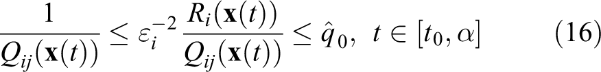
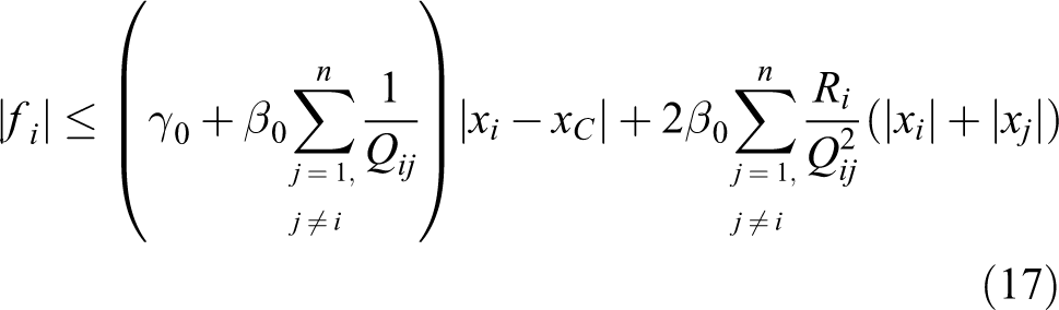
Then with respect to the solution $x(t)$ that exists on $[t_0,\alpha ]$ , we have, therefore, from the inequalities (15) to (18), the estimate, for some constants $k_i>0$ independent of $\alpha$

$\parallel G(x(t))\parallel \le {\displaystyle \sum _{i=1}^n}{k}_i(|x_i(t)|+|y_i(t)|)$

19

It follows from (19), therefore, that for some $M>0$ independent of $\alpha$ , we have the estimate

$\parallel G(x(t))\parallel \le M\parallel x(t)\parallel$

20

which implies that the function $G(x(t))$ is linearly bounded on $[t_0,\alpha ]$ . We shall now show that by this estimate and the comparison theorem the solution can be extended on $[t_0,\infty )$ . To this end, consider again system (4). By taking the inner product of the first equation of (4) and $x(t)$ , we have, by estimate (20)

$\frac{1}{2}\frac{\text{d}}{\text{d}t}\parallel x(t){\parallel }^2=〈\dot{x}(t),x(t)〉=〈G(t),x(t)〉\le \parallel G(x(t))\parallel \cdot \parallel x(t)\parallel \le M\parallel x(t){\parallel }^2$

21

Let $y(t):=\parallel x(t){\parallel }^2$ . Then we have the differential inequality

$\frac{1}{2}\frac{\text{d}}{\text{d}t}y(t)\le My(t),\hspace{0.17em}\hspace{0.17em}y(t_0)=\parallel x_0{\parallel }^2$

22

Comparing (22) and (21), it is easy to see that

$\parallel x(t){\parallel }^2\le \parallel x_0{\parallel }^2{e}^{2M(t-t_0)},\hspace{0.17em}\hspace{0.17em}t\in [t_0,\alpha ]$

23

The a priori boundedness (23) of $\parallel x(t){\parallel }^2$ implies the extension of the solution of (4) on $[t_0,\alpha +\beta ]$ , $\beta >0$ being independent of α. Hence, we are assured of the existence and uniqueness of $x(t)$ in $D(L)$ for all time $t\ge 0$ . It follows therefore that system (4) is well-spaced.

Theorem 6.1

System (4) is well-spaced.

Cohesiveness of system (4)

We establish the cohesiveness of system (4) by proving the boundedness of $x$ about $x_C$ over the domain $D(L)$ . We follow the classical work of Yoshizawa, ²⁶ who worked on the boundedness of solutions with Lyapunov-like functions.

Definition 6.2

The solution $x(t)$ of (4) is equi-bounded about $x_C(t)$ if for every $\lambda >0$ and $t_0\ge 0$ , there exists a $B(t_0,\lambda )>0$ such that if $\parallel x(t_0)-x_C(t_0)\parallel \le \lambda$ , then $\parallel x(t)-x_C(t)\parallel <B(t_0,\lambda )$ for all $t\ge t_0$ .

Definition 6.3

The solution $x(t)$ of (4) is uniformly bounded about $x_C(t)$ if B in Definition 6.2 is independent of $t_0$ .

Lemma 6.4

The solution $x(t)$ of (4) is uniformly bounded about $x_C(t)$ .

Proof

Given $\lambda >0$ and $t_0>0$ , let $x(t)=x(t;t_0,x_0)$ be a solution of (4) in $D(L)$ such that $\parallel x(t_0)-x_C(t_0)\parallel \le \lambda$ . Let ${\gamma }_{\text{min}}:=\text{min}\left\{{\gamma }_1,\dots ,{\gamma }_n\right\}$ , ${\gamma }_{\text{max}}:=\text{max}\left\{{\gamma }_1,\dots ,{\gamma }_n\right\}$ , and ${\epsilon }_{\text{max}}=\text{max}\left\{{\epsilon }_1,\dots ,{\epsilon }_n\right\}$ . Further, define the functions $a(r)$ and $b(r)$ by

$a(r):=\frac{1}{2}{\gamma }_{\text{min}}{r}^2\hspace{0.17em}\hspace{0.17em}\text{and}\hspace{0.17em}\hspace{0.17em}b(r):=\frac{1}{2}{\gamma }_{\text{max}}{r}^2+n{\epsilon }_{\text{max}}^2+L(x(t_0))$

respectively, where L is the Lyapunov-like function given in (7). It is clear that the functions are independent of $t_0$ and $0\le a(r)\le b(r)$ for all $r>0$ . Given that a and b are continuously increasing functions in r and $a,b\to \infty$ as $r\to \infty$ , we can choose a $B=B(\lambda )>0$ so large that

$a(B)>b(\lambda )$

24

We shall now show, by contradiction, that there exists a constant $B(\lambda )>0$ such that if $\parallel x(t_0)-x_C(t_0)\parallel \le \lambda$ , then $\parallel x(t)-x_C(t)\parallel \le B(\lambda )$ for all $t\ge t_0$ . At the onset, we note that since

${\displaystyle \sum _{i=1}^n}{R}_i(x)=\frac{1}{2}\parallel x-x_C{\parallel }^2+{\displaystyle \sum _{i=1}^n}{\epsilon }_i^2$

we have

$a(\parallel x-x_C\parallel )\le L(x)\hspace{0.17em}\hspace{0.17em}\forall x\in {ℝ}^{2n}$

25

Moreover, since ${\stackrel{•}{L}}_{(4)}(x(t))\le 0$ , which implies that

$L(x(t))\le L(x(t_0))\le L(x(0))\hspace{0.17em}\hspace{0.17em}\forall t\ge t_0\ge 0$

26

we can see that

$L(x(t))\le L(x(t_0))\le b(\parallel x(t)-x_C(t)\parallel )\hspace{0.17em}\hspace{0.17em}\forall t\ge 0$

27

Now, assume contrarily that for any $B>\lambda$ , there exists a $t_1\ge t_0$ such that $\parallel x(t_0)-x_C(t_0)\parallel \le \lambda$ but

$\parallel x(t_1)-x_C(t_1)\parallel \ge B(\lambda )$

28

By the continuity of solutions, we can find t′ and t″ such that $t_0\le t^{\prime }\le t″\le t_1$ and

$\parallel x(t^{\prime })-x_C(t^{\prime })\parallel =\lambda \hspace{0.17em}\hspace{0.17em}\hspace{0.17em}\text{and}\hspace{0.17em}\hspace{0.17em}\hspace{0.17em}\parallel x(t″)-x_C(t″)\parallel =B$

Set

$t_1:=\text{sup}\{t^{\prime }:\parallel x(t^{\prime })-x_C(t^{\prime })\parallel =\lambda \}$

and

$t_2:=\text{inf}\{t″:\parallel x(t″)-x_C(t″)\parallel =B\}$

Then $t_1<t_2$

$\parallel x(t_1)-x_C(t_1)\parallel =\lambda ,\hspace{0.17em}\hspace{0.17em}\parallel x(t_2)-x_C(t_2)\parallel =B$

and

$\lambda <\parallel x(t)-x_C(t)\parallel <B\hspace{0.17em}\hspace{0.17em}\forall t\in (t_1,t_2)$

Thus, by (27), we have

$L(x(t_1))\le b(\parallel x(t_1)-x_C(t_1)\parallel )=b(\lambda )$

and by (25)

$a(\parallel x(t_2)-x_C(t_2)\parallel )=a(B)\le L(x(t_2))$

Since $t_1<t_2$ , we have, by (26)

$L(x(t_2))\le L(x(t_1))$

so that

$a(B)\le L(x(t_2))\le L(x(t_1))\le b(\lambda )$

which however clearly contradicts (24) and, thus, our choice of $B(\lambda )$ in (28). Hence $\parallel x(t)-x_C(t)\parallel <B(\lambda )$ for all $t\ge t_0$ . This ends the proof of Lemma 6.4. □

We can now readily establish cohesiveness via Lemma 2.2 and Lemma 6.4.

Theorem 6.5

System (4) is cohesive.

Proof

By Lemma 2.2 and Lemma 6.4, we have that

$r_V<\parallel x(t)-x_C(t)\parallel <\infty \hspace{0.17em}\hspace{0.17em}\forall \hspace{0.17em}\hspace{0.17em}t\ge 0$

Hence both

$\underset{t\to \infty }{{\displaystyle \text{lim}\hspace{0.17em}\mathrm{s}\mathrm{u}\mathrm{p}}}\parallel x(t)-x_C(t)\parallel \hspace{0.17em}\hspace{0.17em}\hspace{0.17em}\text{and}\hspace{0.17em}\hspace{0.17em}\hspace{0.17em}\underset{t\to \infty }{{\displaystyle \text{lim}\hspace{0.17em}\mathrm{i}\mathrm{n}\mathrm{f}}}\parallel x(t)-x_C(t)\parallel$

exist. Now, from the decreasing property of the Lyapunov-like function (7), we have, for all $t\ge 0$

$\frac{1}{2}{\gamma }_{\text{min}}\parallel x-x_C{\parallel }^2<{\displaystyle \sum _{i=1}^n}{\gamma }_i{R}_i(x(t))\le L(x(t))\le L(x(0))$

Thus

$r_V<\parallel x(t)-x_C(t)\parallel \le \sqrt{\frac{2L(x(0))}{{\gamma }_{\text{min}}}}$

Hence, Definition 2.3 is satisfied if we choose

$\overline{K}=\sqrt{\frac{2L(x(0))}{{\gamma }_{\text{min}}}}\hspace{0.17em}\text{and}\hspace{0.17em}\underset{\_}{K}=r_V$

Equilibrium points of system (4)

In this section, we show that system (4) can have equilibrium points, which must correspond to $x$ that solves $\text{d}L/\text{d}t=0$ . In other words, we need to simultaneously solve $f_i(x)=0$ and $g_i(x)=0$ given in (9) and (10), respectively. Now, we note by observation that these equalities hold if $R_i(x)=0$ for all $i=1,\dots ,n$ . However, this means that for some sufficiently small ${\epsilon }_i>0$ , $(x_i,y_i)\approx (x_j,y_j)$ for all $i\ne j$ , $i,j\in \{1,\dots ,n\}$ , at some time $t\ge 0$ . This violates our requirement that $Q_{ij}>0$ or $d_{ij}(t)>2r_V$ at every $t>0$ in $D(L)$ . Hence, we proceed to solve $f_i(x)=0$ and $g_i(x)=0$ with $R_i(x)\ne 0$ . Accordingly, let

${\mathcal{F}}_i:={\gamma }_i+{\displaystyle \sum _{\begin{array}{l}j=1,\\ j\ne i\end{array}}^n\frac{{\beta }_{ij}}{Q_{ij}}}\hspace{0.17em}\hspace{0.17em}\hspace{0.17em}\text{and}\hspace{0.17em}\hspace{0.17em}\hspace{0.17em}{\mathcal{G}}_{ij}:=\frac{2{\beta }_{ij}{R}_i}{Q_{ij}^2}$

29

Then (9) becomes

$\begin{array}{c}{f}_i(x)={\mathcal{F}}_i\hspace{0.17em}(x_i-x_C)-{\displaystyle \sum _{\begin{array}{l}j=1,\\ j\ne i\end{array}}^n{\mathcal{G}}_{ij}\hspace{0.17em}(x_i-x_j)}\\ ={\mathcal{F}}_i\hspace{0.17em}\left(\frac{n-1}{n}{x}_i-\frac{1}{n}{\displaystyle \sum _{\begin{array}{l}j=1,\\ j\ne i\end{array}}^n{x}_j}\right)-{\displaystyle \sum _{\begin{array}{l}j=1,\\ j\ne i\end{array}}^n{\mathcal{G}}_{ij}\hspace{0.17em}(x_i-x_j)}\\ =\left(\frac{(n-1){\mathcal{F}}_i}{n}-{\displaystyle \sum _{\begin{array}{l}j=1,\\ j\ne i\end{array}}^n{\mathcal{G}}_{ij}}\right)x_i-{\displaystyle \sum _{\begin{array}{l}j=1,\\ j\ne i\end{array}}^n\left(\frac{{\mathcal{F}}_i}{n}-{\mathcal{G}}_{ij}\right)x_j}\end{array}$

Then letting $f_i=0$ , we have

$[(n-1){\mathcal{F}}_i-n{\displaystyle \sum _{\begin{array}{l}j=1,\\ j\ne i\end{array}}^n{\mathcal{G}}_{ij}}]x_i-{\displaystyle \sum _{\begin{array}{l}j=1,\\ j\ne i\end{array}}^n[{\mathcal{F}}_i-n{\mathcal{G}}_{ij}]x_j=0}$

30

Similarly, on solving $g_i=0$ , we get

$[(n-1){\mathcal{F}}_i-n{\displaystyle \sum _{\begin{array}{l}j=1,\\ j\ne i\end{array}}^n{\mathcal{G}}_{ij}]}\hspace{0.17em}{y}_i-{\displaystyle \sum _{\begin{array}{l}j=1,\\ j\ne i\end{array}}^n[{\mathcal{F}}_i-n{\mathcal{G}}_{ij}]}{y}_j=0$

31

In solving $f_i=0$ and $g_i=0$ , we want to avoid the trivial solution. Since we only want to know whether we will have equilibrium points, let us consider the special case where

${\mathcal{F}}_i=n{\mathcal{G}}_{ij}\hspace{0.17em}\hspace{0.17em}\mathrm{for all}\hspace{0.17em}\hspace{0.17em}i\ne j$

32

Then the second term of (30) and (31) reduces to zero. The first term also reduces to zero since

$\begin{array}{l}(n-1){\mathcal{F}}_i-n{\displaystyle \sum _{\begin{array}{l}j=1,\\ j\ne i\end{array}}^n{\mathcal{G}}_{ij}}\\ =(n-1){\mathcal{F}}_i-\underset{(n-1)\hspace{0.17em}\mathrm{terms}}{\underbrace{(G_{i1}+G_{i2}+\cdots +G_{ik}+\cdots +G_{in})}}\\ =(n-1){\mathcal{F}}_i-(\underset{(n-1)\hspace{0.17em}\mathrm{terms}}{\underbrace{{\mathcal{F}}_i+\cdots +{\mathcal{F}}_i}})\\ =(n-1){\mathcal{F}}_i-(n-1){\mathcal{F}}_i=0\end{array}$

Now, from (32), we have, if n = 3, for example

${\mathcal{F}}_1=3{\mathcal{G}}_{12},\hspace{0.17em}\hspace{0.17em}{\mathcal{F}}_1=3{\mathcal{G}}_{13},\hspace{0.17em}\hspace{0.17em}{\mathcal{F}}_2=3{\mathcal{G}}_{21},\hspace{0.17em}\hspace{0.17em}{\mathcal{F}}_2=3{\mathcal{G}}_{23},{\mathcal{F}}_3=3{\mathcal{G}}_{31}\hspace{0.17em}\text{and}\hspace{0.17em}{\mathcal{F}}_3=3{\mathcal{G}}_{32}$

which imply that ${\mathcal{G}}_{12}={\mathcal{G}}_{13}$ , ${\mathcal{G}}_{21}={\mathcal{G}}_{23}$ , and ${\mathcal{G}}_{31}={\mathcal{G}}_{32}$ . In general, (32) implies that

${\mathcal{G}}_{ik}={\mathcal{G}}_{ij},\hspace{0.17em}\hspace{0.17em}i,j,k\in \mathbb{N},\hspace{0.17em}\hspace{0.17em}i\ne j,\hspace{0.17em}i\ne k$

33

Equations (32) and (33), therefore, respectively provide us the following important relationships

$\begin{array}{l}{\gamma }_i+{\displaystyle \sum _{\begin{array}{l}j=1,\\ j\ne i\end{array}}^n\frac{{\beta }_{ij}}{Q_{ij}}}=n\frac{2{\beta }_{ij}{R}_i}{Q_{ij}^2}\\ \hspace{1em}\hspace{1em}\hspace{1em}\hspace{1em}\hspace{1em}\frac{{\beta }_{ik}}{Q_{ik}^2}=\frac{{\beta }_{ij}}{Q_{ij}^2},\end{array}\}$

34

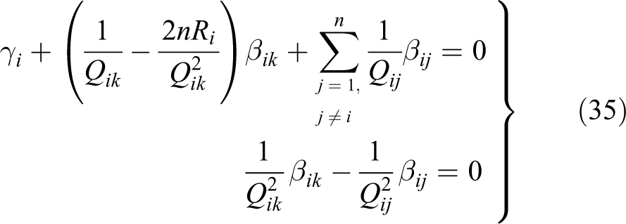
From (34), we can build a homogeneous system of linear equations with respect to the control parameters ${\gamma }_i>0$ , ${\beta }_{ik}>0$ , and ${\beta }_{ij}>0$ , for all $i,j,k\in \mathbb{N}$ , $i\ne j$ , $i\ne k$

$\begin{array}{l}{\gamma }_i+\left(\frac{1}{Q_{ik}}-\frac{2n{R}_i}{Q_{ik}^2}\right){\beta }_{ik}+{\displaystyle \sum _{\begin{array}{l}j=1,\\ j\ne i\end{array}}^n\frac{1}{Q_{ij}}}{\beta }_{ij}=0\\ \hspace{1em}\hspace{1em}\hspace{1em}\hspace{1em}\hspace{1em}\frac{1}{Q_{ik}^2}{\beta }_{ik}-\frac{1}{Q_{ij}^2}{\beta }_{ij}=0\hspace{0.17em}\end{array}\}$

35

or, in matrix notation

$\mathcal{A}y=0$

36

Here, $\mathcal{A}$ is the $n(n-1)\times n^2$ coefficient matrix of system (35). The entries of $\mathcal{A}$ consist of

$1,\left(\frac{1}{Q_{ik}}-\frac{2n{R}_i}{Q_{ik}^2}\right),\frac{1}{Q_{ij}},\frac{1}{Q_{ik}^2} \text{and}\hspace{0.17em} \frac{1}{Q_{ij}^2}$

where the $Q_{ij}$ and R_i are calculated at $x=x_e$ , that is, $\mathcal{A}=\mathcal{A}(x_e)$ . The vector $y$ is an $n^2\times 1$ vector, the entries of which consist of the control parameters $({\gamma }_i,{\beta }_{ij},{\beta }_{ik})$ .

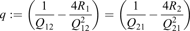
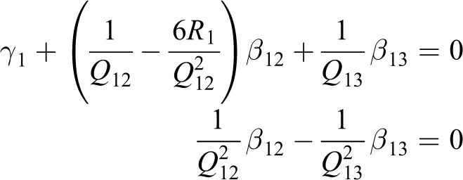
For the case $n=2$ , since $i\ne j$ and $i\ne k$ , which means that $j\ne k$ , system (35) gives

${\gamma }_1+\left(\frac{1}{Q_{12}}-\frac{4R_1}{Q_{12}^2}\right){\beta }_{12}=0 \hspace{0.17em}\mathrm{and}\hspace{0.17em} {\gamma }_2+\left(\frac{1}{Q_{21}}-\frac{4R_2}{Q_{21}^2}\right){\beta }_{21}=0$

37

Consider the special situation where ${\epsilon }_1={\epsilon }_2$ . Then, since $R_1=R_2$ and $Q_{12}=Q_{21}$ for any point $(x_1,y_1,x_2,y_2)\in D(L)$ , we have

$q:=\left(\frac{1}{Q_{12}}-\frac{4R_1}{Q_{12}^2}\right)=\left(\frac{1}{Q_{21}}-\frac{4R_2}{Q_{21}^2}\right)$

Thus

$\mathcal{A}=\left[\begin{array}{cccc}1& q& 0& 0\\ 0& 0& 1& q\end{array}\right] \hspace{0.17em}\text{and}\hspace{0.17em} y={\left[\begin{array}{cccc}{\gamma }_1& {\beta }_{12}& {\gamma }_2& {\beta }_{21}\end{array}\right]}^{\text{T}}$

Now, rank $\mathcal{A}=2<4$ , and nullity $\mathcal{A}=4-2=2$ . The former implies that for every point $x=(x_1,y_1,x_2,y_2)\in D(L)$ that generates q, there are nontrivial solutions $y$ . The latter implies there are two basis vectors for the null space of $\mathcal{A}$ ; they are $(0,0,-q\mathrm{,1})$ and $(-q\mathrm{,1,0,0})$ . Since we want the parameters to be positive, we can add the basis vectors to get $y=({\gamma }_1,{\beta }_{12},{\gamma }_2,{\beta }_{21})=c(-q\mathrm{,1},-q\mathrm{,1})$ for some scalar $c\in ℝ$ . Hence, if we choose $c>0$ , then the point $x=(x_1,y_1,x_2,y_2)$ that makes $q<0$ is an equilibrium point of system (4).

For the case $n=3$ , equation (35) gives, for $i=1$

$\begin{array}{l}{\gamma }_1+\left(\frac{1}{Q_{12}}-\frac{6R_1}{Q_{12}^2}\right){\beta }_{12}+\frac{1}{Q_{13}}{\beta }_{13}=0\\ \hspace{0.5em}\hspace{0.5em}\hspace{0.5em}\hspace{0.5em}\hspace{1em}\frac{1}{Q_{12}^2}{\beta }_{12}-\frac{1}{Q_{13}^2}{\beta }_{13}=0\end{array}$

for $i=2$

$\begin{array}{r}\hfill {\gamma }_2+\left(\frac{1}{Q_{21}}-\frac{6R_2}{Q_{21}^2}\right){\beta }_{21}+\frac{1}{Q_{23}}{\beta }_{23}=0\\ \hfill \frac{1}{Q_{21}^2}{\beta }_{21}-\frac{1}{Q_{23}^2}{\beta }_{23}=0\end{array}$

and for $i=3$

$\begin{array}{l}{\gamma }_3+\left(\frac{1}{Q_{31}}-\frac{6R_3}{Q_{31}^2}\right){\beta }_{31}+\frac{1}{Q_{32}}{\beta }_{32}=0\\ \hspace{0.5em}\hspace{0.5em}\hspace{0.5em}\hspace{1em}\hspace{0.17em}\frac{1}{Q_{31}^2}{\beta }_{31}-\frac{1}{Q_{32}^2}{\beta }_{32}=0\end{array}$

If we let

$\begin{array}{c}{a}_{12}:=\left(\frac{1}{Q_{12}}-\frac{6R_1}{Q_{12}^2}\right),\hspace{0.17em}\hspace{0.17em}{a}_{13}:=\frac{1}{Q_{13}},\hspace{0.17em}\hspace{0.17em}{a}_{22}:=\frac{1}{Q_{12}^2},\hspace{0.17em}\hspace{0.17em}{a}_{23}:=-\frac{1}{Q_{13}^2}\\ a_{35}:=\left(\frac{1}{Q_{21}}-\frac{6R_2}{Q_{21}^2}\right),\hspace{0.17em}\hspace{0.17em}{a}_{36}:=\frac{1}{Q_{23}},\hspace{0.17em}\hspace{0.17em}{a}_{45}:=\frac{1}{Q_{21}^2},\hspace{0.17em}\hspace{0.17em}{a}_{46}:=-\frac{1}{Q_{23}^2}\\ a_{58}:=\left(\frac{1}{Q_{31}}-\frac{6R_3}{Q_{31}^2}\right),\hspace{0.17em}\hspace{0.17em}{a}_{59}:=\frac{1}{Q_{32}},\hspace{0.17em}\hspace{0.17em}{a}_{68}:=\frac{1}{Q_{31}^2},\hspace{0.17em}\hspace{0.17em}{a}_{69}:=-\frac{1}{Q_{32}^2}\end{array}$

then in the form of system (36), we have

$\left[\begin{array}{ccccccccc}1& a_{12}& a_{13}& 0& 0& 0& 0& 0& 0\\ 0& a_{22}& a_{23}& 0& 0& 0& 0& 0& 0\\ 0& 0& 0& 1& a_{35}& a_{36}& 0& 0& 0\\ 0& 0& 0& 0& a_{45}& a_{46}& 0& 0& 0\\ 0& 0& 0& 0& 0& 0& 1& a_{58}& a_{59}\\ 0& 0& 0& 0& 0& 0& 0& a_{68}& a_{69}\end{array}\right]\left[\begin{array}{c}{\gamma }_1\\ {\beta }_{12}\\ {\beta }_{13}\\ {\gamma }_2\\ {\beta }_{21}\\ {\beta }_{23}\\ {\gamma }_3\\ {\beta }_{31}\\ {\beta }_{32}\end{array}\right]=\left[\begin{array}{c}0\\ 0\\ 0\\ 0\\ 0\\ 0\end{array}\right]$

38

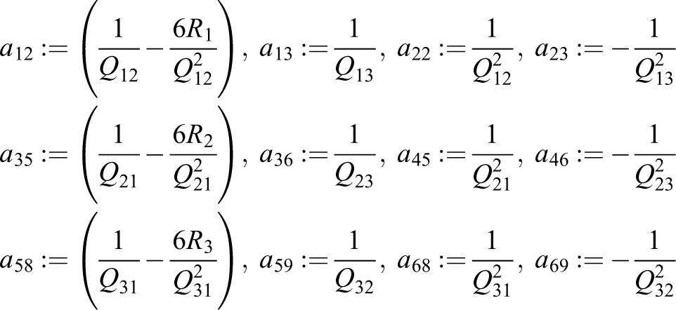
The rank and the nullity of $\mathcal{A}$ are 6 and 3, respectively. Thus, we can conclude that for every point $(x_1,x_2,x_3)\in D(L)$ , we have nontrivial solutions $y$ of system (38). The three basis vectors for the nullspace of $\mathcal{A}$ are

$\begin{array}{l}(\mathrm{0,0,0,0,0,0},-((a_{59}{a}_{68}-a_{58}{a}_{69})/a_{68}),-(a_{69}/a_{68})\mathrm{,1})\\ (0,0,0,-((a_{36}{a}_{45}-a_{35}{a}_{46})/a_{45}),-(a_{46}/a_{45})\mathrm{,1,0,0,0})\\ (-((a_{13}{a}_{22}-a_{12}{a}_{23})/a_{22}),-(a_{23}/a_{22})\mathrm{,1,0,0,0,0,0,0})\end{array}$

which can be added to obtain positive parameters. The points $(x_1,x_2,x_3)\in D(L)$ that produce the positive parameters constitute therefore the equilibrium point $x_e:=(x_1,x_2,x_3)$ of system (4).

In a similar way, we can construct homogeneous systems of linear equations from (35) for higher values of n.

In summary, from equation (35), we can obtain the homogeneous system of linear equations (36), where matrix $\mathcal{A}=\mathcal{A}(x)$ is an $n(n-1)\times n^2$ coefficient matrix whose entries consist of the values of $Q_{ij}$ and R_i at $x$ . The vector $y$ is an $n^2\times 1$ vector of control parameters $({\gamma }_i,{\beta }_{ik},{\beta }_{ij})$ , $i,j,k\in \mathbb{N}$ , $i\ne j$ , $i\ne k$ . Since rank $\mathcal{A}=n(n-1)<n^2$ , the homogeneous system (36) has infinitely many solutions $y$ . Since we want $y>0$ , the n basis vectors of the null space of $\mathcal{A}$ can be added to obtain all positive entries in $y$ . The point $x\in D(L)$ that generates the entries in $\mathcal{A}$ and the positive entries in $y$ such that $\mathcal{A}y=0$ is the equilibrium point $x_e$ of system (4).

Parallel formation in the absence of equilibrium points

In the previous section, when we simultaneously solved $f_i(x)=0$ and $g_i(x)=0$ , we found a solution, namely, a set of equilibrium points. In this subsection, we show that a further analysis produces an unexpected solution—an emergent pattern that so far has only been numerically obtained by other researchers, namely, a highly parallel group, which arises due to the absence of equilibrium points.

Beginning with equations (29), which are

${\mathcal{F}}_i:={\gamma }_i+{\displaystyle \sum _{\begin{array}{l}j=1,\\ j\ne i\end{array}}^n\frac{{\beta }_{ij}}{Q_{ij}}}\hspace{0.17em}\hspace{0.17em} \text{and}\hspace{0.17em} \hspace{0.17em}\hspace{0.17em}{\mathcal{G}}_{ij}:=\frac{2{\beta }_{ij}{R}_i}{Q_{ij}^2}$

we want to solve $f_i(x)=0$ and $g_i(x)=0$ for $x$ , where

$f_i(x)={\mathcal{F}}_i\left(x_i-x_C\right)-{\displaystyle \sum _{\begin{array}{l}j=1,\\ j\ne i\end{array}}^n{\mathcal{G}}_{ij}(x_i-x_j)}$

39

and

$g_i(x)={\mathcal{F}}_i\left(y_i-y_C\right)-{\displaystyle \sum _{\begin{array}{l}j=1,\\ j\ne i\end{array}}^n{\mathcal{G}}_{ij}(y_i-y_j)}$

40

Now, (39) can be written in an expanded form as

$\begin{array}{l}{f}_i(x)={\mathcal{F}}_i\left(x_i-x_C\right)-\underset{n-1 \hspace{0.17em}\mathrm{terms} }{\underbrace{{\mathcal{G}}_{i1}(x_i-x_1)-\cdots -{\mathcal{G}}_{in}(x_i-x_n)}}\\ \hspace{1em}\hspace{0.17em}\hspace{1em}=\left[\frac{{\mathcal{F}}_i}{n}\left(x_i-x_C\right)-{\mathcal{G}}_{i1}(x_i-x_1)\right]+\cdots \\ \hspace{1em}\hspace{1em}\hspace{1em}+\left[\frac{{\mathcal{F}}_i}{n}\left(x_i-x_C\right)-{\mathcal{G}}_{in}(x_i-x_n)\right]\end{array}$

Equation (40) can be written similarly. Thus

$\begin{array}{l}{\stackrel{•}{L}}_{(4)}=-{\displaystyle \sum _{i=1}^n}\left({\mu }_i{f}_i^2+{\phi }_i{g}_i^2\right)\\ \hspace{0.17em}\hspace{0.17em}\hspace{0.17em}=-{\mu }_1\{\frac{{\mathcal{F}}_1}{n}(x_1-x_C)+\left[\frac{{\mathcal{F}}_1}{n}(x_1-x_C)-{\mathcal{G}}_{12}(x_1-x_2)\right]+\cdots \\ {\hspace{1em}+\left[\frac{{\mathcal{F}}_1}{n}(x_1-x_C)-{\mathcal{G}}_{1n}(x_1-x_n)\right]\}}^2\\ \hspace{1em}-{\phi }_1\{\frac{{\mathcal{F}}_1}{n}(y_1-y_C)+\left[\frac{{\mathcal{F}}_1}{n}(y_1-y_C)-{\mathcal{G}}_{12}(y_1-y_2)\right]+\dots \\ {\hspace{0.17em}\hspace{0.17em}+\left[\frac{{\mathcal{F}}_1}{n}(y_1-y_C)-{\mathcal{G}}_{1n}(y_1-y_n)\right]\}}^2-\cdots \\ -{\mu }_n\{\frac{{\mathcal{F}}_n}{n}(x_n-x_C)+\left[\frac{{\mathcal{F}}_n}{n}(x_n-x_C)-{\mathcal{G}}_{n2}(x_n-x_2)\right]+\cdots \\ {\hspace{0.17em}\hspace{0.17em}+\left[\frac{{\mathcal{F}}_n}{n}(x_n-x_C)-{\mathcal{G}}_{n(n-1)}(x_n-x_{n-1})\right]\}}^2\\ -{\phi }_n\{\frac{{\mathcal{F}}_n}{n}(y_n-y_C)+\left[\frac{{\mathcal{F}}_n}{n}(y_n-y_C)-{\mathcal{G}}_{n2}(y_1-y_2)\right]+\dots \\ {\hspace{0.17em}\hspace{0.17em}+\left[\frac{{\mathcal{F}}_n}{n}(y_n-y_C)-{\mathcal{G}}_{n(n-1)}(y_n-y_{n-1})\right]\}}^2\end{array}$

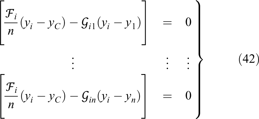
Let us now assume that for certain values of the control parameters ${\gamma }_i>0$ and ${\beta }_{ij}>0$ , we have

$\begin{array}{ccc}\left[\frac{{\mathcal{F}}_i}{n}\left(x_i-x_C\right)-{\mathcal{G}}_{i1}(x_i-x_1)\right]& =& 0\\ ⋮& ⋮& ⋮\\ \left[\frac{{\mathcal{F}}_i}{n}\left(x_i-x_C\right)-{\mathcal{G}}_{in}(x_i-x_n)\right]& =& 0\end{array}\}$

41

and

$\begin{array}{ccc}\left[\frac{{\mathcal{F}}_i}{n}\left(y_i-y_C\right)-{\mathcal{G}}_{i1}(y_i-y_1)\right]& =& 0\\ ⋮& ⋮& ⋮\\ \left[\frac{{\mathcal{F}}_i}{n}\left(y_i-y_C\right)-{\mathcal{G}}_{in}(y_i-y_n)\right]& =& 0\end{array}\}$

42

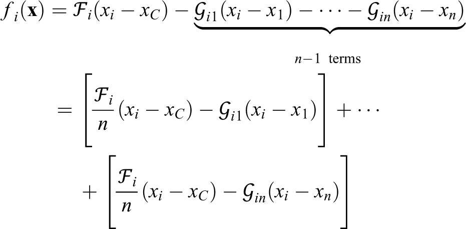
We can thus solve (41) and (42) simultaneously to get an equilibrium point $x_e$ . For the i th case, we need to simultaneously solve the four equations

$\begin{array}{r}\frac{{\mathcal{F}}_i}{n}\left(x_i-x_C\right)=0\\ \frac{{\mathcal{F}}_i}{n}\left(x_i-x_C\right)-{\mathcal{G}}_{ij}(x_i-x_j)=0\\ \frac{{\mathcal{F}}_i}{n}\left(y_i-x_C\right)=0\\ \frac{{\mathcal{F}}_i}{n}\left(y_i-y_C\right)-{\mathcal{G}}_{ij}(y_i-y_j)=0\end{array}\}$

43

noting that the first and third equations come from the fact that ${\mathcal{G}}_{ii}(x_i-x_i)={\mathcal{G}}_{ii}(y_i-y_i)=0$ . From these equations, since ${\mathcal{F}}_i\ne 0$ and ${\mathcal{G}}_{ij}\ne 0$ in $D(L)$ , it must be that $(x_i,y_i)=(x_C,y_C)$ and $(x_i,y_i)=(x_j,y_j)$ , for all $i,j\in \{1,\dots ,n\}$ , $i\ne j$ . This implies that an equilibrium point must be where all the individuals collapse onto each other. However, this is impossible in $D(L)$ . Hence, it must be that $(x_i,y_i)\ne (x_C,y_C)$ and $(x_i,y_i)\ne (x_j,y_j)$ , for all $i,j\in \{1,\dots ,n\}$ , $i\ne j$ . Thus, we are left with only the second and forth equations to solve simultaneously

$\begin{array}{l}\frac{{\mathcal{F}}_i}{n}\left(x_i-x_C\right)-{\mathcal{G}}_{ij}(x_i-x_j)=0\\ \frac{{\mathcal{F}}_i}{n}\left(y_i-y_C\right)-{\mathcal{G}}_{ij}(y_i-y_j)=0\end{array}\}$

44

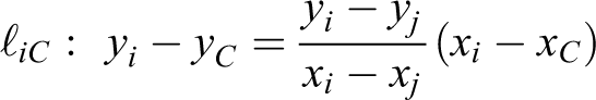
This is solvable to give the set of lines

$S:=\{x\in D(L):(x_i-x_j)(y_i-y_C)-(y_i-y_j)(x_i-x_C)=0\}$

for all $i,j=1,2,\dots ,n$ , $i\ne j$ . Consequently, in $D(L)$ , if (44) holds, then

${\stackrel{•}{L}}_{(4)}=-{\displaystyle \sum _{i=1}^n}\left\{{\mu }_i{\left[\frac{{\mathcal{F}}_i}{n}(x_i-x_C)\right]}^2+{\phi }_i{\left[\frac{{\mathcal{F}}_i}{n}(y_i-x_C)\right]}^2\right\}<0$

which also tells us, since ${\stackrel{•}{L}}_{(4)}\ne 0$ , there is no equilibrium point in $D(L)$ in the special case where (44) holds. In conclusion, since a line in S can be written as

${\ell }_{iC}:\hspace{0.17em}\hspace{0.17em}{y}_i-y_C=\frac{y_i-y_j}{x_i-x_j}(x_i-x_C)$

or

${\ell }_{ij}:\hspace{0.17em}\hspace{0.17em}{y}_i-y_j=\frac{y_i-y_C}{x_i-x_C}(x_i-x_j)$

we can encounter two possible scenarios.

Line ${\ell }_{iC}$ tells us that any point mass A_i can be on the same line that joins its position $(x_i,y_i)$ to the position of the centroid $(x_C,y_C)$ . Its slope is equal to $(y_i-y_j)/(x_i-x_j)$ , the slope of a line that would have existed if A_i and A_j were on it. This simply means that at least one point mass will be on ${\ell }_{iC}$ while the rest of the point masses will be on other lines parallel to ${\ell }_{iC}$ .

Similarly, line ${\ell }_{ij}$ tells us that at least two point masses A_i and A_j will be on a line parallel to a line whose slope is $(y_i-y_C)/(x_i-x_C)$ and which would have existed if A_i and the centroid were on it. The other members of the group will be on lines parallel to ${\ell }_{ij}$ .

Other researchers have reported this type of emergent behavior using their swarm model. For example, Couzin et al. ²⁷ described this behavior as is an instance of highly parallel group, which is a group that self-organizes into a highly aligned arrangement with rectilinear motion. The same behavior is reported in Liu et al. ²⁸ and Xue et al. ²⁹ However, these papers only manage to numerically generate the pattern. Our result gives a first explicit formulation of the pattern.

Application to planar mobile car-like vehicles

In this section, we apply our method of developing the Lagrangian swarm model to design the velocity controllers of autonomous car-like robots. We reproduce the description of the robots from the authors’ work in Vanualailai et al., ³⁰ starting with Figure 5 which shows the i th car-like with front wheel steering and engine power applied to the rear wheels. For each car i, let $\xi >0$ be the distance between the two axles and $\ell >0$ the length of each axle. Assuming that ${\varphi }_i={\theta }_i$ , the kinematic model of the car-like robot with respect to its center $(x_i,y_i)\in {ℝ}^2$ is, as shown in Pappas and Kyriakopoulos ³¹

${\stackrel{•}{x}}_i={\upsilon }_i\text{cos}{\theta }_i-\frac{\xi }{2}{\omega }_i\text{sin}{\theta }_i,\hspace{0.17em}\hspace{0.17em}{\stackrel{•}{y}}_i={\upsilon }_i\text{sin}{\theta }_i+\frac{\xi }{2}{\omega }_i\text{cos}{\theta }_i,\hspace{0.17em}\hspace{0.17em}{\stackrel{•}{\theta }}_i={\omega }_i$

45

where the variable θ_i gives the robot’s orientation with respect to the $z_1$ -axis of the $z_1$ – $z_2$ coordinates, and υ_i and ω_i are the instantaneous translational and angular velocities, respectively. To ensure that the i th vehicle safely steers pass other vehicles, we enclose it by the smallest circle possible. As shown in Figure 5, if we let ${\epsilon }_1>0$ and ${\epsilon }_2>0$ be the clearance parameters, then we can enclose the vehicle by a protective circular region centered at $(x,y)$ , with radius $r_V:=\sqrt{{(2{\epsilon }_1+\xi )}^2+{(2{\epsilon }_2+\ell )}^2}/2$ . We can thus take equation (1) as the definition of our car-like robots. Accordingly, our system consists of the robots A_i as members of a swarm. The centroid of the swarm is given by (2). Our objective is to design the translational velocities υ_i and the angular velocities ω_i such that robots are attracted to the centroid as a cohesive and well-spaced swarm.

Figure 5.

The i th planar mobile robot which is car-like, with front wheel steering and steering angle ϕ_i.

Velocity controllers for the vehicles

Let us extend the definition of the independent variable from $x_i=(x_i,y_i)\in {ℝ}^2$ to $q_i:=(x_i,y_i,{\theta }_i)\in {ℝ}^3$ , and $q:=(q_1,\dots ,q_n)\in {ℝ}^{3n}$ . Then (45) is the i th component of the system

$\stackrel{•}{q}=H_1(q)v+H_2(q)w,\hspace{0.17em}\hspace{0.17em}{q}_0:=q(t_0)$

46

where $v:=({\upsilon }_1,\dots ,{\upsilon }_n)\in {ℝ}^n$ , $w:=({\omega }_1,\dots ,{\omega }_n)\in {ℝ}^n$ , and $H_1$ and $H_2$ are $3n\times n$ matrices defined as

$H_1=\left[\begin{array}{cccccc}\text{cos}{\theta }_1& 0& 0& \cdots & 0& 0\\ \text{sin}{\theta }_1& 0& 0& \cdots & 0& 0\\ 0& 0& 0& \cdots & 0& 0\\ 0& \text{cos}{\theta }_2& 0& \cdots & 0& 0\\ 0& \text{sin}{\theta }_2& 0& \cdots & 0& 0\\ 0& 0& 0& \cdots & 0& 0\\ ⋮& ⋮& \ddots & \ddots & \ddots & ⋮\\ 0& 0& 0& \cdots & 0& 0\\ 0& 0& 0& \cdots & 0& \text{cos}{\theta }_n\\ 0& 0& 0& \cdots & 0& \text{sin}{\theta }_n\\ 0& 0& 0& \cdots & 0& 0\end{array}\right]$

and

$H_2=\left[\begin{array}{cccccc}-\frac{\xi }{2}\text{sin}{\theta }_1& 0& 0& \cdots & 0& 0\\ \frac{\xi }{2}\text{cos}{\theta }_1& 0& 0& \cdots & 0& 0\\ 1& 0& 0& \cdots & 0& 0\\ 0& -\frac{\xi }{2}\text{sin}{\theta }_2& 0& \cdots & 0& 0\\ 0& \frac{\xi }{2}\text{sin}{\theta }_2& 0& \cdots & 0& 0\\ 0& 1& 0& \cdots & 0& 0\\ ⋮& ⋮& \ddots & \ddots & \ddots & ⋮\\ 0& 0& 0& \cdots & 1& 0\\ 0& 0& 0& \cdots & 0& -\frac{\xi }{2}\text{sin}{\theta }_n\\ 0& 0& 0& \cdots & 0& \frac{\xi }{2}\text{cos}{\theta }_n\\ 0& 0& 0& \cdots & 0& 1\end{array}\right],$

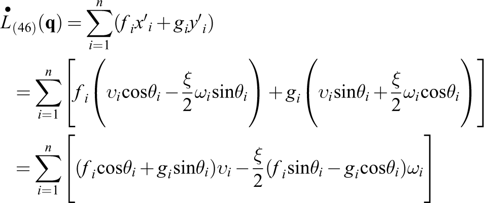
respectively. We can use $R_i=R_i(q)$ defined in (5) for the attraction to the centroid and $Q_{ij}=Q_{ij}(q)$ defined in (6) for interindividual collision avoidance. Then applying the Lyapunov-like function (7) to system (46) over the domain

$\tilde{D}(L):=\left\{q\in {ℝ}^{3n}:Q_{ij}(q)>0\hspace{0.17em}\forall \hspace{0.17em}i,j=1,\dots ,n,i\ne j\right\}$

we have, noting that $\partial L/\partial {\theta }_i=0$ since L does not contain a function of θ_i, and using $f_i$ and $g_i$ defined in (9) and (10), respectively

$\begin{array}{l}{\stackrel{•}{L}}_{(46)}(q)={\displaystyle \sum _{i=1}^n}(f_i{x^{\prime }}_i+g_i{y^{\prime }}_i)\\ ={\displaystyle \sum _{i=1}^n}\left[f_i\left({\upsilon }_i\text{cos}{\theta }_i-\frac{\xi }{2}{\omega }_i\text{sin}{\theta }_i\right)+g_i\left({\upsilon }_i\text{sin}{\theta }_i+\frac{\xi }{2}{\omega }_i\text{cos}{\theta }_i\right)\right]\\ ={\displaystyle \sum _{i=1}^n}\left[\left(f_i\text{cos}{\theta }_i+g_i\text{sin}{\theta }_i\right){\upsilon }_i-\frac{\xi }{2}\left(f_i\text{sin}{\theta }_i-g_i\text{cos}{\theta }_i\right){\omega }_i\right]\end{array}$

Accordingly, we can define the steering control laws as

${\upsilon }_i:=-k_i\left(f_i\text{cos}{\theta }_i+g_i\text{sin}{\theta }_i\right)\hspace{0.17em} \text{and}\hspace{0.17em} \hspace{0.17em}{\omega }_i:=\frac{2k_i}{\xi }\left(f_i\text{sin}{\theta }_i-g_i\text{cos}{\theta }_i\right),$

47

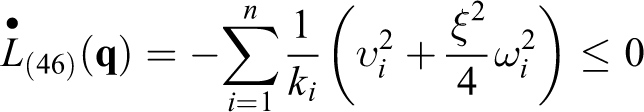
where we want $k_i$ to be some arbitrary positive function of $x_i$ and $y_i$ only, and differentiable over $\tilde{D}(L)$ . With these control laws, we have, with respect to system (46)

${\stackrel{•}{L}}_{(46)}(q)=-{\displaystyle \sum _{i=1}^n}\frac{1}{k_i}\left({\upsilon }_i^2+\frac{{\xi }^2}{4}{\omega }_i^2\right)\le 0$

With (47), system (45) simplifies to

${\stackrel{•}{x}}_i=-k_i{f}_i,\hspace{0.17em}\hspace{0.17em}{\stackrel{•}{y}}_i=-k_i{g}_i,\hspace{0.17em}\hspace{0.17em}{\stackrel{•}{\theta }}_i=\frac{2k_i}{\xi }\left(f_i\text{sin}{\theta }_i-g_i\text{cos}{\theta }_i\right)$

48

The first two equations in (48) are independent of θ_i. That is, the positions $(x_i,y_i)$ are determined by $k_i>0$ , $f_i$ , and $g_i$ , which are functions of $x_i$ and $y_i$ only. Hence, it is sufficient to study the reduced system

${\stackrel{•}{x}}_i=-k_i{f}_i,\hspace{0.17em}\hspace{0.17em}{\stackrel{•}{y}}_i=-k_i{g}_i,\hspace{0.17em}\hspace{0.17em}{x}_{i0}:=x_i(t_0),\hspace{0.17em}\hspace{0.17em}{y}_{i0}:=y_i(t_0),\hspace{0.17em}\hspace{0.17em}{t}_0\ge 0$

49

and let it the be the i th component of the system

$\stackrel{•}{x}=F(x),\hspace{0.17em}\hspace{0.17em}{x}_0=x(t_0)$

50

where $F(x):=(-k_1(x)f_1(x),-k_1(x)g_1(x),\dots ,-k_n(x)f_n(x),-k_n(x)g_n(x))\in {ℝ}^{2n}$ . Since we are supposing that $k_i\in C^1[\widehat{D}(L),{ℝ}_{+}]$ , ${ℝ}_{+}:=(0,\infty )$ , where

$\widehat{D}(L):=\left\{x\in {ℝ}^{2n}:Q_{ij}(x)>0\hspace{0.17em}\forall \hspace{0.17em}i,j=1,\dots ,n,i\ne j\right\}$

system (50) has the same form and property as system (4). It is therefore well-spaced and cohesive in $\widehat{D}(L)$ .

Restrictions on velocities and steering angles

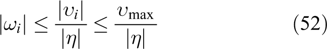
A practical consideration is the mandatory restrictions on the velocities and the steering angle. In our case, the function $k_i=k_i(x)>0$ plays an important role restricting the size of the steering angles φ_i. To see this, let ${\upsilon }_{\text{max}}:={{\displaystyle \text{max}}}_{i\in \mathbb{N}}|{\upsilon }_i|$ and ${\varphi }_{\text{max}}:={{\displaystyle \text{max}}}_{i\in \mathbb{N}}|{\varphi }_i|$ , with $0<{\varphi }_{\text{max}}<\pi /2$ . As shown in Pappas and Kyriakopoulos, ³¹ the relationship between the translational velocities, υ_i, and the angular velocities, ω_i, is governed by

${\upsilon }_i^2\ge {\eta }^2{\omega }_i^2 \hspace{0.17em}\mathrm{where}\hspace{0.17em}\hspace{0.17em}\eta :=\frac{\xi }{\text{tan}{\varphi }_{\text{max}}}$

51

From (51), we easily have

$|{\omega }_i|\le \frac{|{\upsilon }_i|}{|\eta |}\le \frac{{\upsilon }_{\text{max}}}{|\eta |}$

52

Now, given any constant $\psi \ge 1$ , we have, from (47)

$|{\upsilon }_i|\le k_i\left(\psi +|f_i|+|g_i|\right) \hspace{0.17em}\text{and}\hspace{0.17em} |{\omega }_i|\le \frac{2k_i}{\xi }\left(\psi +|f_i|+|g_i|\right)$

53

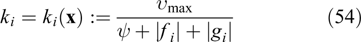
If we set $k_i:={\upsilon }_{\text{max}}$ , for instance, then the first inequality in (53) holds. Further, the second inequality in (53) and the inequality (52) are consistent if we let

$\frac{2k_i}{\xi }=\frac{2v_{\text{max}}}{\xi }=\frac{{\upsilon }_{\text{max}}}{|\eta |}$

from which we get $|\eta |=\xi /2$ . Thus, from (51), we have $\text{tan}{\varphi }_{\text{max}}=2$ and ${\varphi }_{\text{max}}={{\displaystyle \text{tan}}}^{-1}2$ . In other words, if we set $k_i={\upsilon }_{\text{max}}$ , then the maximum steering angle of every vehicle is set at ${\varphi }_{\text{max}}={{\displaystyle \text{tan}}}^{-1}2$ .

In our simulations, we shall illustrate that an appropriately chosen $k_i=k_i(x)$ that is continuous on $\widehat{D}(L)$ and satisfies (53) is sufficient to induce swarming with emergent patterns. If we choose, for example

$k_i=k_i(x):=\frac{{\upsilon }_{\text{max}}}{\psi +|f_i|+|g_i|}$

54

we can also show, along similar arguments as the above, that ${\varphi }_{\text{max}}={{\displaystyle \text{tan}}}^{-1}2$ .

Simulations

For our simulations, we use the first two terms, ${\stackrel{•}{x}}_i$ and ${\stackrel{•}{y}}_i$ in (48) to obtain the positions $(x_i(t),y_i(t))$ of the i th vehicle, and the third term ${\stackrel{•}{\theta }}_i$ to obtain its orientations, ${\theta }_i(t)$ , at time $t>0$ . At time $t=0$ , the initial positions $(x_{i0}(0),y_{i0}(0))$ and orientations ${\theta }_i(0)$ are randomly generated. The vehicles are drawn as arrows, with the arrowhead indicating the front of the vehicles. In each simulation, we use the following parameters:

Clearance parameters: ${\epsilon }_1={\epsilon }_2=0.1$ ;

Width and length of vehicle: $\ell =1$ , $\xi =2$ ;

Radius of circular protective region: $r_V=1.25$ ;

Maximum speeds and steering angle: ${\upsilon }_{\text{max}}={\omega }_{\text{max}}=2$ , ${\varphi }_{\text{max}}={{\displaystyle \text{tan}}}^{-1}2$ ;

$\psi =1$ in (53).

Additionally, since theoretically we require that $k_i\in C^1[\widehat{D}(L),{ℝ}_{+}]$ , we can choose $k_i=k_i(x)={\upsilon }_{\text{max}}$ as suggested in the previous section. However, we shall use (54) to illustrate that it is sufficient that $k_i$ is continuous on $\widehat{D}(L)$ to induce emergent patterns.

With the above parameters fixed, the remaining parameters are the cohesive parameters ${\gamma }_i>0$ and the coupling parameters ${\beta }_{ij}>0$ , for $i,j=1,2,\dots ,n$ . As discussed in the “Roles of the parameters in the Lyapunov-like function” section, the cohesive parameters provide the strength of attraction between individuals and the coupling parameters provide the strength of repulsion between individuals.

We will consider two examples, each with only five vehicles to clearly illustrate the behavior of each vehicle. The first example illustrates the existence of an equilibrium point, while the second example illustrates the absence of one.

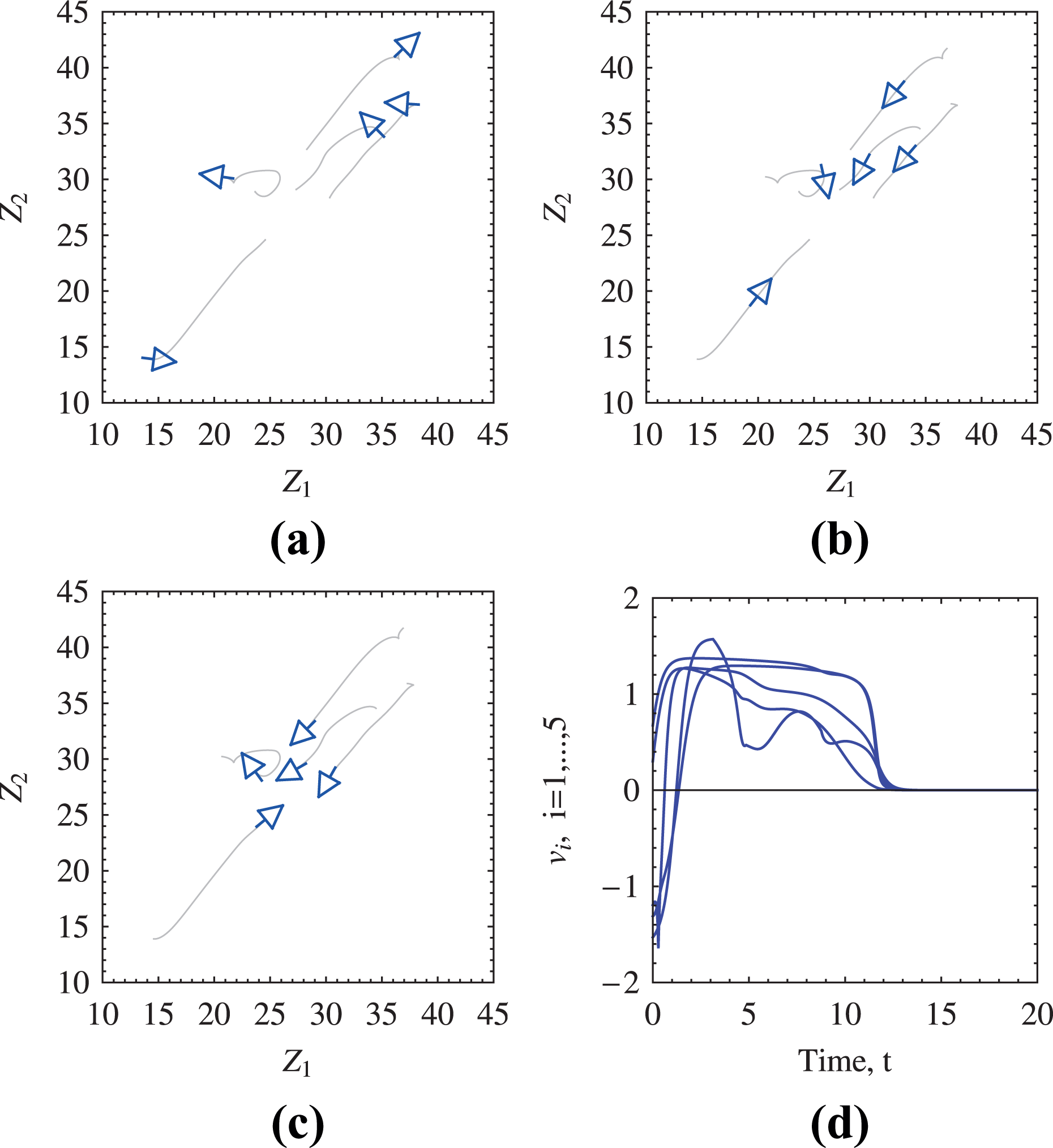
Example 9.1 (constant arrangement about a stationary centroid)

The parameters, for all $i,j=1,2,3,4,5$ , are ${\gamma }_i=1$ and ${\beta }_{ij}=1$ . The emergent pattern is a stationary arrangement about the centroid (Figure 6).

Figure 6.

(a) Randomized initial positions and orientations of five vehicles. (b) At $t=7$ , the vehicles are seen converging toward the centroid. We see that the top-most vehicle and the second vehicle from the left have to reverse to align correctly. (c) By $t=20$ , the vehicles are stationary. Their trajectories are shown as lighter lines. (d) The instantaneous translational velocities eventually become zero, and, as expected, $|{\upsilon }_i|\le {\upsilon }_{\text{max}}=2$ for all $t\ge 0$ and $i=1,\dots \mathrm{,5}$ .

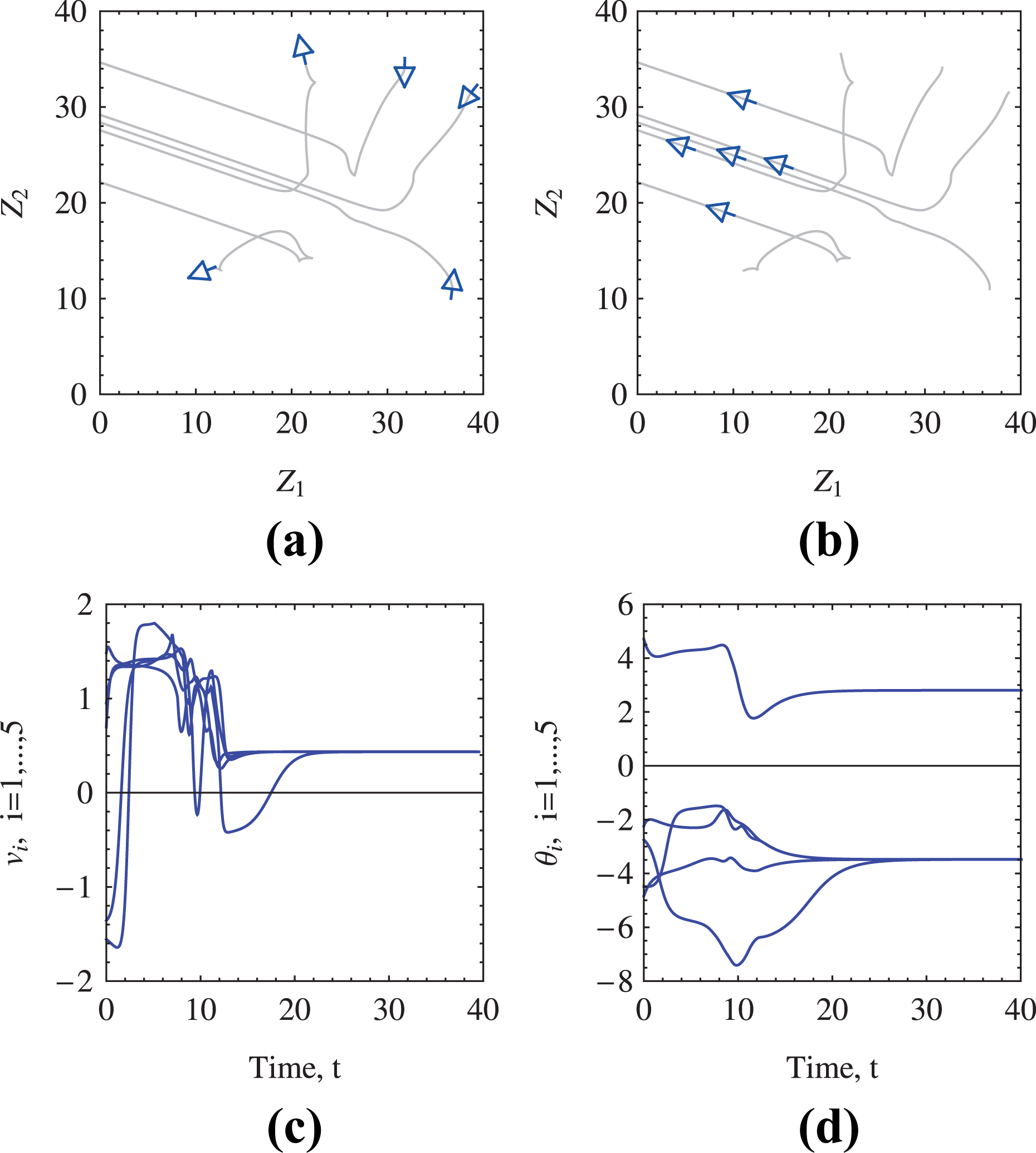
Example 9.2 (highly parallel formation)

In this example, the parameters, for all $i,j=1,2,3,4,5$ , are γ_i randomized between and including 1 and 2, and ${\beta }_{ij}=10$ . The emergent pattern is a parallel formation wherein the distances between the vehicles eventually stabilize over time (Figure 7).

Figure 7.

(a) Randomized initial positions and orientations of five vehicles. (b) By time $t=40$ , the vehicles are seen in parallel formation. Their trajectories are shown in gray. (c) The instantaneous translational velocities converge to a common velocity, with $|{\upsilon }_i|\le {\upsilon }_{\text{max}}=2$ . (d) The angles θ_i of the vehicles stabilize with time.

Conclusion

In individual-based or Lagrangian swarm models governed by systems of first-order ordinary differential equations, the global existence and uniqueness of solutions, and the boundedness of solutions about the centroid of the swarm, are important properties. They ensure that the swarm model is cohesive and well-spaced.

This article developed a Lagrangian swarm model on the hypothesis that animal swarming is an interplay between long-range attraction and short-range repulsion between the individuals in the swarm. It treated both cohesive and well-spaced notions in a rigorous manner. The existence, uniqueness, and boundedness of solutions about the centroid were established via a Lyapunov-like function with attractive and repulsive components.

Extensive simulations suggested that the proposed artificial Lagrangian swarm model was sufficiently general to induce several stable patterns recognized as outcomes of collective behavior or self-organization. These are (a) constant arrangements about a stationary centroid, (b) parallel formations, (c) circular or oscillatory formations about a fixed point, and (d) random walks. To the author’s knowledge, such generality is not seen in other similar Lagrangian swarm models including the most recent one proposed in Li. ¹⁸ The different types of emergent patterns arise by varying the system parameters.

This article, therefore, has provided a means to develop a generalized swarm model that could be used in engineering applications that seek to induce cooperation and pattern formation among multiple autonomous robotic agents.