
Abstract
For robots with flexible joints, the joint torque dynamics makes it difficult to control. An effective solution is to carry out a joint torque controller with fast enough dynamic response. This article is dedicated to design such a torque controller based on sliding mode technique. Three joint torque control approaches are proposed: (1) The proportional-derivative (PD)-type controller has some degree of robustness by properly selecting the control gains. (2) The direct sliding mode control approach which fully utilizes the physical properties of electric motors. (3) The sliding mode estimator approach was proposed to compensate the parameter uncertainties and the external disturbances of the joint torque system. These three joint torque controllers are tested and verified by the simulation studies with different reference torque trajectories and under different joint stiffness.
Introduction
A robot manipulator with flexible joints 1 –3 is normally not intended by the robot designer. Joint flexibility is a side effect when achieving a relative lightweight, for example, for space or medicine applications. Therefore, how to treat the joint torque dynamics makes the different control approaches for this kind of robots.
During the past decade, various methods have been proposed in order to control flexible joint robots. Theoretically, there is a general approach to control flexible joint robots (a large class of nonlinear systems) which is able to achieve fast response as well as “high bandwidth,” namely the state-space approach based on the feedback linearization, 4,5 though some of nonlinear systems are not feedback linearizable. The disadvantage of this approach is the need for higher order time derivatives of the system output (i.e. the variable to be controlled). For the case of flexible joint robots, from the second time derivative of the link position one can only see the joint torque. And, from the fourth time derivative of the link position one can see the motor current. Only from the fifth time derivative of the link position one can see the final system control input, namely the stator voltage of the electric motor. Therefore, for the control design using the state-space approach, one needs up to the fourth time derivatives of the link position signal. As a result, the state-space approach based on the feedback linearization is not adequate for the control of flexible joint robots.
Another methodology to control flexible joint robots is to decompose the high-order system into two or more lower order subsystems. One of the control methods under this category is the cascaded control method. 6 It is well known that for classical cascaded control, the reference input to the inner control loop must be kept “constant” (means changing slowly) during the convergence of the inner control loop, implying that the response time of the total control system is slowed down due to the cascaded structure, resulting in a lower bandwidth with respect to the state-space approach. This is the price one has to pay for the advantages of the cascaded control method. The latter approach is the famous singular perturbation approach 7,8 as well as the integral manifold approach 9 which takes the joint torque subsystem as an algebraic system for the link position control and adds some damping to the fast mode in the joint torque.
In addition, other methods have also been proposed for flexible joint robot control, such as integral backstepping approach, 10 passivity-based control approach, 11 adaptive control technique, 12 fuzzy logic and neural network approaches, 13 and simple PD (or proportional-integral-derivative (PID)) control. 14 However, most of these control methods focus on position control and pay little attention to joint torque dynamics.
As mentioned in the study by Amjadi et al., 15 singular perturbation approach is a smart solution to handle the joint torque dynamics. However, singular perturbation approach does not possess the tracking capability to follow a joint torque trajectory and it is only a solution based on some practice considerations. And now the question may arise: Why the tracking capability to follow a joint torque trajectory is required? Firstly, the composite control structure based on singular perturbation approach as well as integral manifold approach, viewed as a standard control structure for flexible joint robots, has the feature of open-loop control of joint torque dynamics, thus lack of robustness. This weakness has been observed by some researchers. 16 For example, if the joint stiffness changes, the controller based on singular perturbation approach does not possess the mechanisms to follow this change. Secondly, for a high-performance force or impedance control with a reasonable dynamic response in end-effector coordinate frame, the joint torque tracking capability is necessary. Imagining that an end-effector is grasping a moving workpiece, the control system must have a fast enough dynamic response, and the joint torque tracking controller will make this possible. Moreover, the dynamic motion of human arms is actually based on the joint torque feedback (thinking on an extreme case when a blind person touches his environment).
As a result, joint torque tracking capability is important for the control of a high-performance flexible joint robot. Though it is a difficult task to design a robust joint torque controller, joint torque control characterizes the main difference between the classic control and the modern control of flexible joint robots. Sliding mode control approach is the promising control approaches for the control of real-world high-order, nonlinear, multiple-input and multiple-output uncertain system, such as flexible joint robots and nonholonomic constrained mobile robots, 17 –19 because they introduce proper physical information or utilize the physical property of controlled plant to make the solution simple and effective, rather than to play mathematical games. It is pointed out that modern sliding mode control theories have great potential to the control problems in this area. So, in this article, three different joint torque controllers based on sliding mode technique for multiple-link flexible joint robots will be proposed, verified, and compared by simulation studies.
Dynamic model
The model of a flexible joint robot manipulator with n degrees of freedom can be written as

where
Taking joint torque τ and link position q as state variables, model (1) can be reformulated as

The second equation of equation (2) represents the joint torque dynamics. Note that from the first equation of equation (2) we know

It seems that the above equation about the joint torque is decoupled; this is because that the coupling effects from the other joints are acted through the joint acceleration
In order to see the dynamic behavior of the joint torque more clearly,

where


Since matrix M(q)−1 is not a diagonal matrix, we can see the coupling effects:
The disturbance vector Dτ
(t) contains all time-varying parameters of robot arm through term
The joint torque dynamics of one joint are influenced by the joint torques of all other joints through matrix Aτ (t), implying that the joint torques are interconnected between the joints.
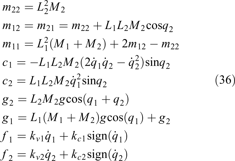
Taking a two-link flexible joint robot as an example, the joint torque dynamics for the two joints can be derived as

where z = 1/(m 11 m 22 − m 12 m 21). Note that parameters mij and ni (with i =1, 2 and j =1, 2) are time-varying.
For the decentralized joint torque control design, it is preferred to use model (3), because of the simplicity. Since parameter uncertainties and unknown disturbances exist, robust control approaches are necessary.
Joint torque control by PD controller
For the analysis of the PD type of joint torque controller for the ith joint, model (3) is cleaned by removing subscript i (keep in mind that we now deal with the torque control of one joint, i.e. the decentralized joint torque control problem)

We know that motor torque τm is generated by the motor stator current iq with the relation τm = ktiq , with kt being the torque constant of the permanent magnet synchronous motor (PMSM) used for the joint. So that the actual control input of the torque dynamics is the motor stator current iq , that is

Now the control task is: Look for the reference current

where eτ
= τd
− τ is the torque control error and
However, since the resulting reference current
For the inner current control loop, either the conventional PWM technique or PD current control can be used. For the simulation studies given in this article the latter is used. Note that for the joint torque control we need only to control the stator current component iq
, but current component id
has influence to the control of iq
. For the joint torque control purpose, we will set the reference current
Joint torque control by direct sliding mode control
In the previous section, we discussed the cascaded control structure for the joint torque control, with inner current control loop and outer PD-type joint torque control loop. This control structure has some advantages, namely:
the designs of the joint torque control and the current control can be done separately;
it is easier for the implementation and for the tuning of the controller parameters; and
only first time derivative of the joint torque signal is required.
However, there are some disadvantages with this simple control system:
The cascaded control structure limits the bandwidth of the closed-loop system.
The system robustness is limited.
The torque control system will not work properly if the joint torque dynamics are faster than the ones of motor current, this will happen when the joint stiffness is high, that is, the robot is more rigid.
Large chattering may occur if the control gains of the PD controller are too high.
In the following, we propose a direct (non-cascaded) joint torque control schema without using the conventional PWM, which is dedicated to overcome these disadvantages. The proposed new control schema has the following features:
It fully utilizes the property of electric motors, namely, the final control signals of the power converter (i.e. inverter) have to be discontinuous, no matter which control strategy is employed and no matter which state variables of the robot are controlled.
The inner current control loop for the q-component is removed. This motor current component is then implicitly controlled through the control of the second time derivative of the joint torque, resulting in a state-space control schema, thus increasing the system bandwidth.
The stability of the closed-loop torque tracking control system can be proved and the robustness with respect to the system uncertainties can be guaranteed.
As control design tool, we use again the sliding mode control theory. The system model used for the decentralized joint torque control for ith joint (subscript i is removed for simplicity) is given as

where ωe
is the rotor electrical angular speed, and the relation with the joint angular speed

with P being the number of pole pair of the PMSM and

Taking the time derivative of the first equation in equation (11) and substituting with the second equation result in the third-order model for the joint torque related to the stator voltage uq

Then, the system model (dynamics about the joint torque τ and about the stator current component id ) can be given as

where the following auxiliary parameters are introduced in order to simplify the notation

Note that in the second equation of equation (13), both sides are multiplied with A −1, such that both stator voltages ud and uq in equation (13) have the same coefficient, this will simplify the controller design.
Controller design
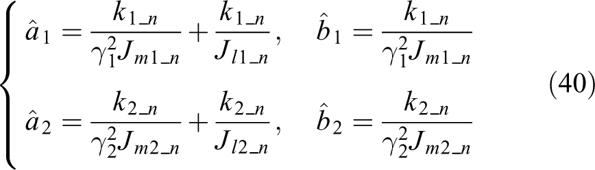
At first, the switching functions for the joint torque and for the d-component of the state current are designed see Appendix 1, Fig.A2

where eτ = τd − τ is the joint torque control error. Note that the parameter A− 1 L is introduced in sd to simplify the control design. The controller will depend on this parameter any way, when not multiplied here, it must be involved in the sliding mode transformation given later.
The time derivative of both switching functions along the solutions of equation (13) can be derived as

Introducing two auxiliary variables fτ and fd as follows

Equation (16) will be simplified to

Note that for these two auxiliary variables,

From the study by Ademi and Jovanović, 20 we know that the stator voltages ud and uq are not yet the discontinuous voltages applied to the motor windings. For the direct sliding mode control design, we need the relation between the final discontinuous voltages applied to the motor windings and the time derivative of both switching functions. This relation can be found by using the definition given in
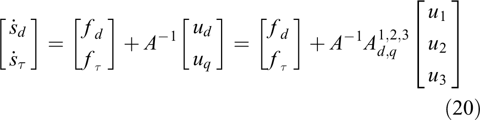
where matrix

With θa = θe , θb = θe − 2π/3, θc = θe + 2π/3 and θe being the rotor electrical angular position. Depending on equation (21), equation (20) can be rewritten as

To find the control signals u 1, u 2, and u 3, Lyapunov approach will be employed. Design a Lyapunov function candidate as

where
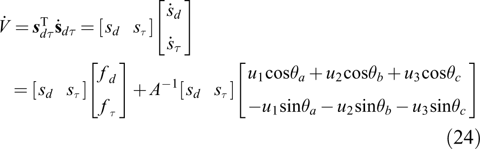
Equation (24) can be further expanded as

Introducing three additional auxiliary variables

Equation (25) can be simplified to

Equation (26) can be interpreted as a kind of sliding mode transformation which performs actually the decoupling task for multi-inputs control systems, see also Utkin et al. 21 for more details. If sd = 0 and sτ = 0, that is, sliding mode occurs, then Ω i = 0 (i = 1, 2, 3) as well.
In order to guarantee
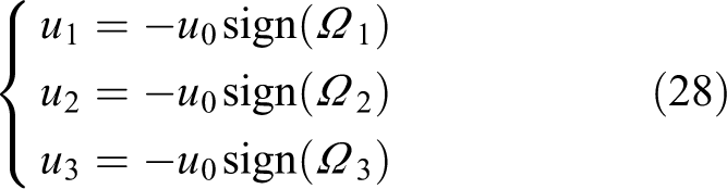
where u 0 is the DC-bus voltage of the inverter. With these control signals, equation (27) can be reformulated for the final analysis

In the above equation, A
−1 is a positive constant (but may not be known). If the scalar term (sdfd
+ sτfτ
) is bounded and if the DC-bus voltage u
0 is high enough,
the DC-bus voltage u 0 should be high enough, and
auxiliary variables fτ and fd are bounded.
Since fτ
and fd
do not contain the control voltages, neither ud
and uq
nor u
1, u
2, and u
3, the condition (b) is reasonable. Actually, only term
Implementation steps
Though the derivation of the proposed control system looks rather sophisticated, the implementation of the controller is quite simple. Step 1: Calculating the joint torque error and the switching functions

Step 2: Calculating the sliding mode transformation

with θa = θe , θb = θe − 2π/3, θc = θe + 2π/3.
Step 3: Calculating the discontinuous control voltages

In equation (30), parameters c
0 and c
1 have to be provided by the control designer depending on the required closed-loop performance of the joint torque control. Parameter A
−1
L = kγkt
/J is not easy to obtain and thus can be tuned, until
Joint torque control by SME
The dynamic model about the joint torques, that is, equation (4) (which is in matrix–vector form) can be rewritten in component-wise for the ith robot joint (here again, subscript i is not used for simplicity)

As discussed in the “Dynamic model” section, a(t) is a function of the components of the robot mass matrix M(q), and d(t) is a function of the components of all dynamic terms in the first equation of equation (1) and a function of the joint torques of all other joints, see also equation (5) as an example. We assume that parameters a(t), d(t), and b in equation (33) are unknown, but bounded. For the implementation of the control algorithm, we need a rough estimate (or called nominal value) of a(t) and b, denoted as
where
This joint torque controller needs an inner current control loop. Same as the “Joint torque control by PD controller” section, we will use the direct sliding mode current controller in the current control loop for the simulation study. The reference q-axis current feeding to the current controller is calculated by
Simulation studies
Plant model used for the simulation
To verify the proposed control approaches, we use a two-link flexible joint robot as the plant model, which consists of the two-link rigid-body robot model can be given as

with
where kvi and kci (i =1, 2) are coefficients of viscous friction and coulomb friction, respectively.
The joint model given by the second and third equations of equation (1), the PMSM model in the AC-form and the voltage transformation were given by Ademi and Jovanović. 20 The final control inputs are the discontinuous control voltages applied to the three stator windings, that is u 1, u 2, and u 3, taking values from the discrete set {−u 0, +u 0}.
The parameters of the two-link flexible joint robot used for the simulation are listed in Tables 1
to 3. Note that for the simulation, the joint disturbance torque in equation (1) is selected as
Arm parameters.

Parameters for motor 1 and motor 2.

Parameters of joint 1 and joint 2.

Reference inputs for testing the joint torque controllers
Three types of torque reference are fed to each of the three joint torque controllers:
step input of 10 Nm with the step time at t = 0,
4 Hz sinusoidal input with 10 Nm amplitude for the case of small signal tracking, and
4 Hz sinusoidal input with 100 Nm amplitude for the case of large signal tracking.
To test the robustness of the joint torque controllers, the joint stiffness of both robot joints in the plant model is changed from 10,000 Nm/Rad to 1000Nm/Rad and the reference signals for the simulation are repeated from point (a) to point (c), in order to verify the behavior of the joint torque controllers in the case of very large joint compliance without changing the controller parameters.
Controller parameters
The parameters for the all three joint torque controllers are tuned to have a satisfactory torque control response for the case of step reference torque input of 10 Nm (i.e. point (a)). And then, these parameters remain unchanged for the all other simulation tests.
For the joint torque controller given in the “Joint torque control by PD controller” section, that is, the PD controller, only three parameters for each joint are required, kp
, kd
, and
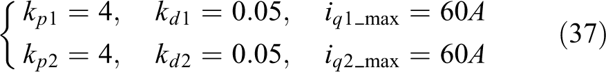
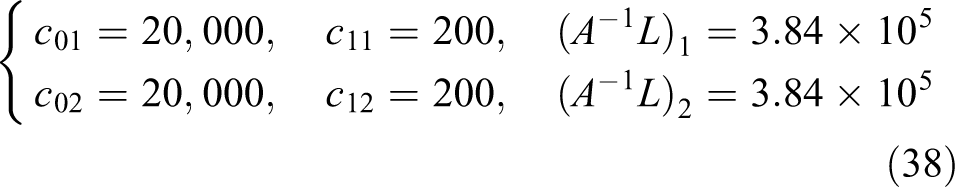
For the joint torque controller given in the “Joint torque control by direct sliding mode control” section, that is, the direct sliding mode control approach, we also need three parameters for each joint, c 0, c 1, and A −1 L = kγkt /J, see equation (30). Actually, parameter A −1 L is dedicated for the construction of the sliding surface for the control of stator current id component (while stator current iq component is not explicitly controlled). Simulation shows that the joint torque control system is not sensitive to this parameter, this result coincides with the theoretical expectation by the author. For the simulation, the controller parameters are selected as
For the control approach given in the “Joint torque control by SME” section, that is, the SME approach, some nominal parameters are required for the pole placement of the torque tracking control. These parameters are selected artificially to have some derivation with respect to their true counterparts (because their true values are actually unknown in practice).
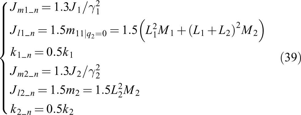
where
Other controller parameters required for this joint torque controller are c 0, c 1, Ms , and the time constant of the low-pass filter. They are selected as
where μ 1 and μ 2 are the time constant of the both low-pass filters for both robot joints.
Theoretically, both the direct sliding mode control approach and the SME approach possess the torque tracking control property. The former needs less controller parameters but the second time derivative of the joint torque signal, while the latter needs only the first time derivative of the joint torque signal but much more controller parameters. Thus, there is always some price to pay for a high control performance. As to the differences in the dynamic response of the both joint torque controllers, refer the discussions given below.
Simulation results and discussions
Figures 1 to 6 show the simulation results of the three joint torque controllers applied to the two-link flexible joint robot considering the AC-motor dynamics.

Step response of joint torque control: (a) response of joint 1 and (b) joint 2.

Sinusoidal torque reference (small amplitude): (a) response of joint 1 and (b) joint 2.

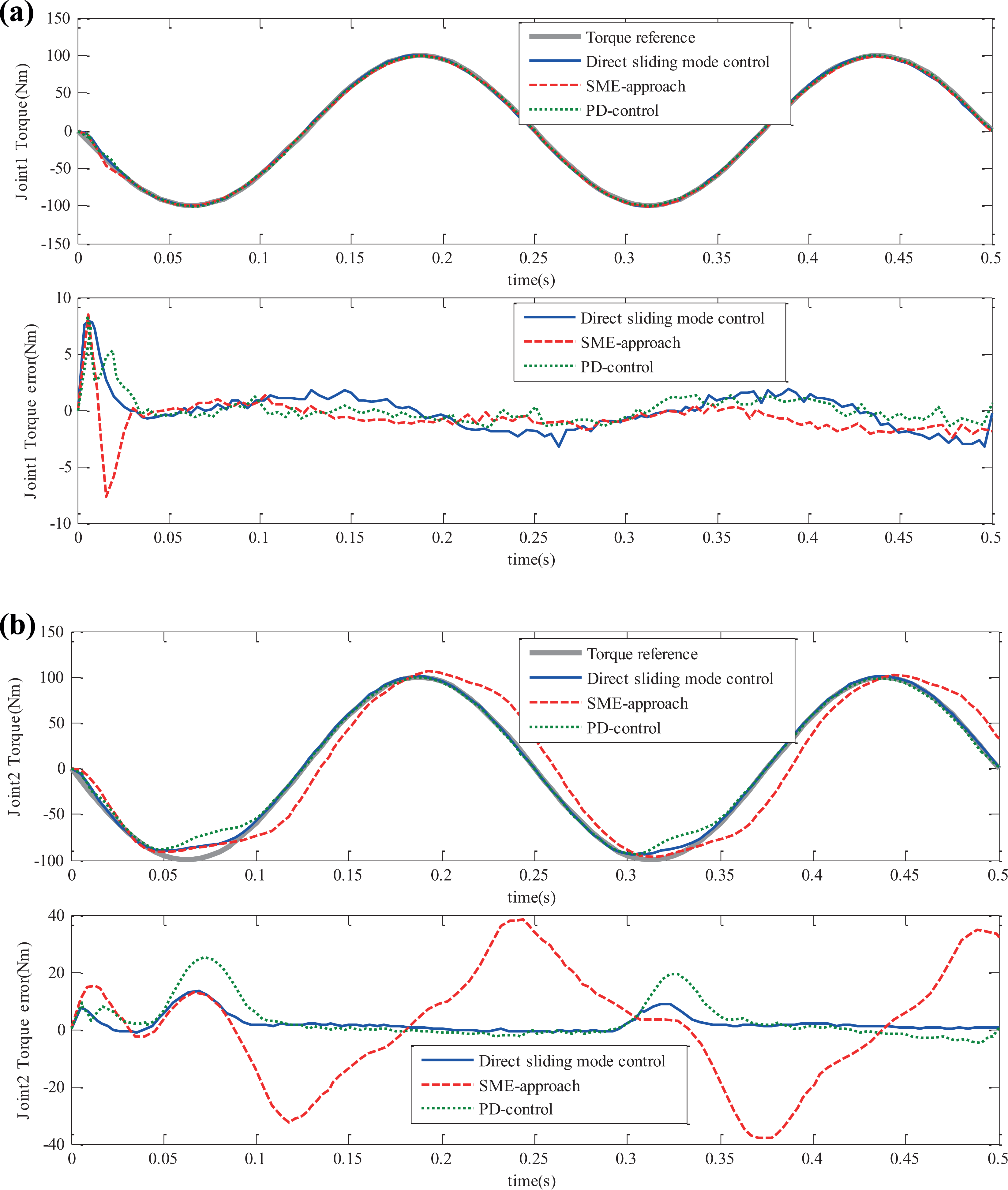
Sinusoidal torque reference (large amplitude): (a) response of joint 1 and (b) joint 2.

Step response of joint torque control (very large joint compliance): (a) response of joint 1 and (b) joint 2.

Sinusoidal torque reference (small amplitude, very large joint compliance): (a) response of joint 1 and (b) joint 2.
Sinusoidal torque reference (large amplitude, very large joint compliance): (a) response of joint 1 and (b) joint 2.
Figures 1 to 3 are for the case of normal flexible joint robots with both joint stiffness k 1 = k 2=10,000. From Figure 1, we see that the step responses of the direct sliding mode control approach and the SME approach are similar, they converge fast and smoothly to the reference value. The step response of the PD control is a little bit slower and not smooth during the transition phase. The control gains of the PD-controller are set so that the possible fast step response can be reached (just before vibrations occur). For the sinusoidal torque reference of small amplitude (see Figure 2), all three control approaches have similar performance. For the sinusoidal torque reference of large amplitude (see Figure 3), the PD control is unusable, this is because that the PD-control results in a too large and fast changing reference current for the inner current control loop which cannot be followed by the current controller. The SME approach has a time delay in the torque response, see the plot for joint 2 in Figure 3. Among the three control approaches, the direct sliding mode control approach has the best tracking control performance for the case of large sinusoidal torque reference. This result matches the expectation of the author.
Figures 4
to 6 are for the case of the flexible joint robots with very large joint compliance, that is, very low joint stiffness k
1 = k
2 = 1000. For the simulations in this category, all other parameters in the controllers and in the plant model remain the same as in the case of normal joint stiffness (i.e. k
1 = k
1 =10,000). The step responses of the PD control and the direct sliding mode control, see Figure 4, have no noticeable change with respect to the case of normal joint stiffness (comparing with Figure 1). Now the step response of the SME approach has an overshoot, see the plot for joint 2 in Figure 4. As mentioned before, the SME approach needs the nominal value of some parameters, if these nominal values differ from their true values too much and the controller parameters (including
Conclusions
This article focuses on the joint torque control problems for flexible joint robots. It is emphasized here again that joint torque is a well-selected state variable for the dynamic control issues of this kind of robots, though the control design and implementation is a difficult task. With the decentralized joint torque control schema, the robot dynamics are decoupled (between robot arm and robot joints). Thus, the results for the control of rigid-body arms can be used further. Three joint torque control approaches are proposed: (1) The PD-type controller has some degree of robustness by properly selecting the control gains. (2) The direct sliding mode control approach which fully utilizes the physical properties of electric motors. (3) The SME approach was proposed to compensate the parameter uncertainties and the external disturbances of the joint torque system. These three joint torque controllers are tested and verified by the simulation studies with different reference torque trajectories and under different joint stiffness. As expected, the direct sliding mode control approach showed the best control performance, but for the control implementation, the second time derivative of the joint torque signal is required. The SME approach tries to avoid the second derivative of joint torque signal, but possesses a more involved control structure and needs more controller parameters; and it generates a time delay when tracking a reference torque signal with large amplitude. The PD-type joint torque controller may become unstable.
Footnotes
Declaration of conflicting interests
The author(s) declared no potential conflicts of interest with respect to the research, authorship, and/or publication of this article.
Funding
The author(s) disclosed receipt of the following financial support for the research, authorship, and/or publication of this article: This project is supported by the National Natural Science Foundation of china (NSFC) [Grant Nos. 61763030, 61263045, 51265034], Jiangxi Province Science and Technology Support Project [Grant No. 20112BB550017], and the Jiangxi Province Natural Science Fund Project [Grant No. 20132BAB201040].
Appendix 1
The proof of stability process is as follows:
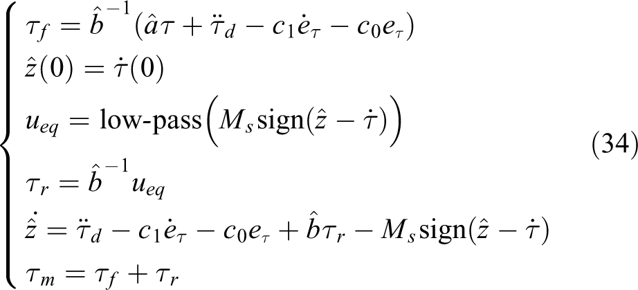
Design control τf as
where
The left-hand side of equation (1B) is linear with poles determined by c 0, c 1 > 0, but is subjected to the perturbation term
which may be simplified by substitution of
In order to improve the control performance, the disturbance (1D) should be compensated for by the additional disturbance rejection term τr in τm = τf + τr . Because τp is immeasurable, an estimate can be obtained using a sliding mode observer of the form
with
Here,
where
The control discontinuity, denoted by the signum function sign() in equation (1F), is introduced along the observation error
Stability of the observer system is ensured via Lyapunov function candidate
where
Because observer (1E) is calculated in the control computer, the initial condition can be set as
such that
In order to estimate the disturbance torque τp
to be compensated via disturbance rejection term τr
in τm
= τf
+ τr
, the equivalent control method, see Utkin,
1
is exploited here once again. In sliding mode, we have
The control signal u in equation (1F) contains two components: a high-frequency switching component resulting from the discontinuous signum term and a low-frequency component, that is, the equivalent control u
eq. As discussed in detail in Utkin,
1
the equivalent control is equal to the average value of u, obtained by a low-pass filter. With this in mind,
leads to a closed-loop error dynamics
where uav can be obtained by a low-pass filter with the discontinuous control u given in (1F) as the filter input.
Hence, sliding mode estimator τr
successfully rejects both the uncertainties in parameters a and b, and the additive disturbance d in equation (33) and allows controller (1A) to perform exact pole placement. It should be noted that the time constant or the bandwidth of the low-pass filter has to be carefully chosen: to be faster than the perturbation dynamics given by equation (1C) for a successful rejection of τp
, but at the same time slow enough to avoid exciting unmodeled dynamics (e.g. the neglected actuator dynamics). In practical applications, since the spectrum of the perturbation dynamics does not come into the spectrum of the high-frequency switching (after sliding mode occurs), a trade-off can normally be found for the selection of the filter time constant. It should be pointed out that for this SME design, only the first time derivative of the joint torque signal is required, whereas the approach given by Elmali and Olgac
2
would need the second time derivative of the joint torque. Moreover, there is no need to assume that the time-derivative of the system perturbation is equal to zero. Utkin VI. Sliding modes in control and optimization. London, UK: Springer-Verlag, 1992. Elmali H and Olgac N. Theory and implementation of sliding mode control with perturbation estimation. In: Proceedings of the IEEE ICRA’92, Nice, France, 12–14 May 1992, pp. 2114–2119. IEEE.