The application of computational fluid dynamics simulation technique to ocean boat anti-disturbance tracking controller

Abstract

This article presents the verification problem of estimating boat hull damping parameters using the computational fluid dynamics technique. In addition, a Lyapunov-based path control system will be introduced to centify the estimation result. The controller should satisfy the following features: firstly, maintaining that the boat dynamic model which includes path, velocity, and orientation errors are asymptotically stable; secondly, ensuring the actuation is operating normally under the nonlinear hydrodynamic system and actual environment limitation; thirdly, working with the anti-disturbance algorithm which includes a projection update law. The final part of the article introduces the procedure proving that the computational fluid dynamics simulation result and Lyapunov direct method controller are acceptable for the ocean boat nonlinear dynamic system. It is confirmed that the control system simulation can improve computational fluid dynamics technology instead of an actual experiment. It can solve the estimation problem caused by limitations in equipment or funds.

Introduction

Ocean boat hull hydrodynamic parameters are usually estimated by towing tank, a kind of huge and expensive equipment. A towing tank had lots of requirements in terms of electrical power or working space. ¹ Therefore, hydrodynamic testing experiments are usually done by computer-based simulation technique named computational fluid dynamics (CFD) instead of actual equipments. The ocean ship hydrodynamic CFD simulation technology in development for many years. One of the most famous CFD experiments was done by the US Navy. The simulation target was a warship named DTMB5415. ^2,3 During the research process, a finite elements analysis technique was used to estimate the nonlinear damping coefficients. After a boundary micro-meshing process, the hydro-force between the ship’s hull and the ocean was able to be simulated by ANSYS software. The final result denoted that ship “cut” ocean water inordinately at different speeds. The damping parameters were also simulated by micro-meshed parts on the ship’s hull boundary. There are also some similar methods and experiments mentioned in the study by Banks et al. ⁴ and Brennen. ⁵ However, there was a problem with CFD simulation—that the results cannot been certified effectively until compared with an actual experiment. In this article, the certification research was based on a nonlinear control system. In other words, if the ship controller worked properly, the CFD simulation produced a successful result.

For driving unmanned surface vehicles (USV), there were many suitable control algorithms such as Proportional–Integral–Derivative (PID), Linear-Quadratic Regulator (LQR), and Backstepping. ^{6 –8} As usual, PID controllers were widely used in vessels’ control systems. There are many papers about the application of PID controller to vessels, such as a ship control model with two multilayer neural networks hydrodynamic estimator ⁹ and a patrol vessel heading control system. ¹⁰ The LQR controller is an automated way of finding an appropriate state-feedback controller; for example, an ocean submarine control system ¹¹ that solved the time delay problem. Backstepping is a recursive process terminated when its subsystems are built from an irreducible stabilized system. Such as a torpedo MIMO backstepping control system ¹² to track a trajectory generated by a way-point guidance system. In the case of autonomous underwater vehicles (AUV) named INFANTE ^{13 –15} made by Instituto Superior Técnico, Lisbon, Portugal, a new methodology was proposed for the design of path following systems. A nonlinear control strategy achieved global convergence to reference paths by taking explicitly into account the dynamics of the vehicle. ^16,17 In another backstepping control project is about underactuated ship models ¹⁸ which includes two propellers without sway force.

This study was conducted to solve the CFD estimation effectiveness problem. The solution involves Lyapunov direct method and backstepping controller. The research target was a unmanned surface vehicle (USV) named Q-boat which worked under ocean current turbulence. The mathematics symbols are introduced in the second section. In the third section, the ocean boat dynamic kinematic models are introduced in detail. Following on in the fourth section, the boat hydrodynamic parameters are simulated by CFD technique based on ANSYS software. ^{19 –21} However, the simulation results could not be substituted in the control system directly. It was necessary that analyzing the data efficiency and cancelling failure numbers before building up the mathematics model. In the fifth section, a nonlinear controller was introduced step by step in detail. For an actual ocean boat moving on a 2-D surface, a backstepping controller solved the unmanned aerial vehicle (UAV) autonomous model driving problem by the Lyapunov direct method. Generally speaking, the controller developing procedure is based on the three steps of position, velocity, and acceleration. It was a hard research topic about controlling an autonomous model, such as a hovercraft ²² and a quadrotor. ²³ There were also disturbance estimation laws in each Lyapunov tentative step respectively. The methodology was based on geometry projection law, which was usually used on estimations of unknown parameters. ^{24 –27} The simulation result is exhibited in the sixth section. The position, velocity, and acceleration errors converged to equilibrium value, which showed that the controller was working properly. The disturbance estimation result also demonstrated that the projection update law was suitable for hydrodynamic model noise cancellation. Finally, in conclusion, the article presents that the effectiveness of boat hydrodynamic CFD estimation can be certificated by USV backstepping control system. Moreover, a future study project was introduced that a practical USV driving experiment based on Robot Operation System (ROS) and accurate global positioning system (GPS) navigation equipments.

Notation

In this article, the prime $f^{\prime }(x)$ denotes the partial derivative of the function f with respect to x, such as $f^{\prime }(x)=\frac{\partial f}{\partial x}(x)$ . The upper dot $\dot{f}(x)=f^{\prime }(x(t))\dot{x}(t)$ denotes total time derivative of the function f. Symbol $e_i$ denotes the ith unitary vector. For example, ${\mathbf{e}}_1,{\mathbf{e}}_2,{\mathbf{e}}_3$ represent the vector ${[1,0,0]}^{\text{T}}$ , ${[0,1,0]}^{\text{T}}$ , and ${[0,0,1]}^{\text{T}}$ respectively. Boldface letter 1 denotes unit vector ${[1,\mathrm{1...1}]}^{\text{T}}$ . When describing an unknown variable x, $\widehat{x}$ represents the estimation of x and $\tilde{x}$ denotes the error between real x and estimated $\widehat{x}$ value. In this article, a boat’s motion is related with an inertial reference frame $\left\{I\right\}$ and a body-fixed frame $\left\{B\right\}$ . For transforming the coordinate from body $\left\{B\right\}$ into inertial $\left\{I\right\}$ , there is a rotation matrix $R\in \text{SO}\left(\text{3}\right)$ which is about boat’s orientation $\psi$ . When calculating the time derivative of rotation matrix R, there is a sym-skew matrix S which satisfied the following function

$\frac{\text{d}R(\psi )}{\text{d}t}=RS(\dot{\psi })$

A function $\sigma (s):ℝ\to ℝ$ is a saturation function if it is differentiable and verifiable, for positive M and ${\sigma }_{\text{max}}$

$\begin{array}{l}0<{\sigma }^{\prime }(s)<M,\text{for} \text{all} s,\\ -\sigma (s)=\sigma (-s),\text{for} \text{all} s,\\ s\sigma (s)>0,\text{for} \text{all} s\ne 0,\sigma (0)=0,\\ \underset{s\to \pm \infty }{{\displaystyle \text{lim}}}\sigma (s)=\pm {\sigma }_{\text{max}}\end{array}$

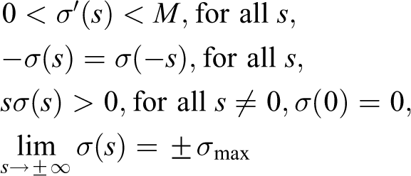
Examples of smooth saturation functions are ${\sigma }_1(s)=s/\sqrt{1+s^2}$ and ${\sigma }_2(s)=\text{arctan}(s)$ .

Ocean boat model

The boat’s coordinates

In this case, the experiment platform is a marine boat named Q-boat, which is specifically designed for test algorithm about ocean USV cooperation control and sea-bed scanning, as shown in Figure 1.

Figure 1.

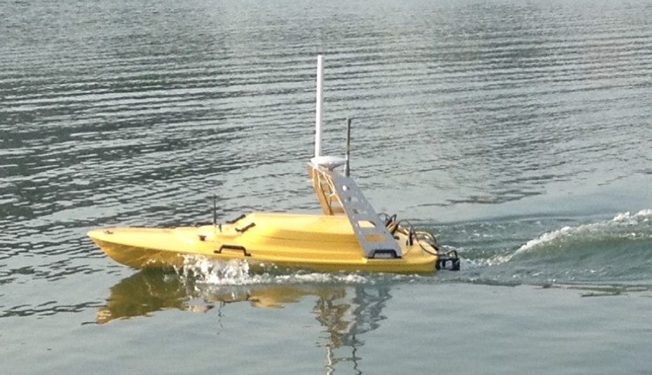
Q-boat testing in the ocean.

A boat model includes its statics and dynamics functions. ^{7,18,28 –31} According to professor Fossen’s classical ocean engineering textbook, ³² a ship model includes the motion in 6 degrees of freedom (DOF) which are named surge, sway, heave, roll, pitch, and yaw, as shown in Figure 2. The first three describe the position motion along $x,y$ , and z axis, while, the last three are about orientation and rotation motion.

Figure 2.

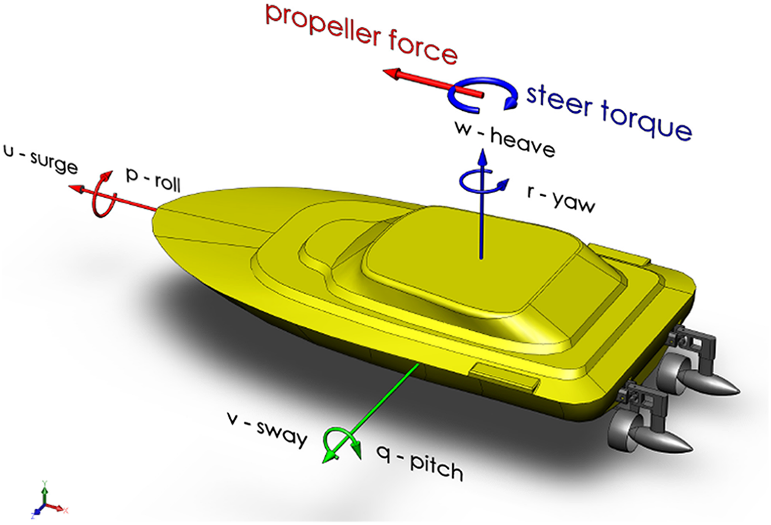
Q-boat coordinations.

Boat kinematics equations

For the boat model in this case, the heave, pitch, and roll modes which represent boat moving in the vertical plane are neglected. Therefore, the boat kinematics equations are

$\dot{\mathbf{p}}=R(\psi )\mathbf{v}$

1

$\dot{\mathbf{o}}=\mathit{\omega }$

2

where $\dot{\mathbf{p}}$ is position vector, ${[x y z]}^{\text{T}}$ , with $z=0$ ; $\dot{\mathbf{o}}$ is orientation vector, ${[\varphi \theta \psi ]}^{\text{T}}$ , with $\varphi =\theta =0$ ; $R(\psi )\in {ℝ}^3$ is a rotation matrix about orientation angle ψ; $\mathbf{v}\in {ℝ}^3$ is linear velocity vector, ${[u \mathbf{v} 0]}^{\text{T}}$ ; and $\mathit{\omega }\in {ℝ}^3$ is angular velocity vector, ${[0 0 r]}^{\text{T}}$ .

Boat dynamic equations

The boat dynamic equation of motion can be conveniently expressed as

$m\dot{\mathbf{v}}=\mathbf{t}-S(\mathit{\omega })m\mathbf{v}-D(\parallel \mathbf{v}\parallel )\mathbf{v}+m{R}^{\text{T}}\mathbf{b}$

3

$(I_{zz}-N_{\dot{r}})\dot{r}={\tau }_r-N_{r}r-N_{|r|r}|r|r$

4

where m is the mass scalar; $\mathbf{t}\in {ℝ}^3$ is the propeller force, ${[{\tau }_u 0 0]}^{\text{T}}$ ; $D(\parallel \mathbf{v}\parallel )\mathbf{v}$ is nonlinear damping force; R is rotation matrix; $\mathbf{b}$ is unknown disturbance; ${\tau }_r$ is boat rudder torque; $I_{zz}$ is boat inertia moment; $\dot{r}$ is angular acceleration; $N_r$ and $N_{|r|r}$ are linear and nonlinear damping moment parameters.

It is necessary for the model to simplified before higher-order calculation. Firstly, because a normal boat satisfies the following condition equation (5), the boat inertia moment $I_{zz}$ and added mass $N_{\dot{r}}$ parameters are unequal

$I_{zz}-N_{\dot{r}}\ne 0$

5

Secondly, based on boat kinematics equation (1) and dynamic equation (3), the boat acceleration is

$\ddot{\mathbf{p}}=\mathbf{t}-\frac{1}{m}RD(\parallel \mathbf{v}\parallel )\mathbf{v}+\mathbf{b}$

6

where nonlinear damping part is a diagonal matrix. Each element includes the norm of the velocity, as follows

$\begin{array}{l}D(\parallel \mathbf{v}\parallel )=\text{diag}\left[\begin{array}{c}a,a,a\end{array}\right]\\ a=\frac{X_u+Y_v+X_u}{3}+\frac{X_{|u|u}+Y_{|v|v}+X_{|u|u}}{3}\parallel \mathbf{v}\parallel \end{array}$

7

Finally, the error between actual and ideal acceleration is

$\begin{array}{l}{\ddot{\mathbf{p}}}_e=\ddot{\mathbf{p}}-{\ddot{\mathbf{p}}}_c\\ =R(M_c^{-1}{D}_c(\parallel \mathbf{v}\parallel )-M^{-1}D(\parallel \mathbf{v}\parallel ))\mathbf{v}\\ \hspace{1em}\hspace{1em}+R(S(\mathit{\omega })-M^{-1}S(\mathit{\omega })M)\mathbf{v}\end{array}$

8

where S is a sym-skew matrix as introduced before.

CFD estimation technology

Basic boat data

Based on the manual books, ^{19 –21} ANSYS is used to simulate nonlinear damping coefficients in the Q-boat case. Similar with methods in the literature, ^1,4,5 the boat was firstly simplified as an uniform density ellipsoid. The boat’s mass is 25 kg, radius dimensions are $a=0.901\hspace{0.17em}\text{m},\hspace{0.17em}b=0.450\hspace{0.17em}\text{m},\hspace{0.17em}c=0.150\hspace{0.17em}\text{m}$ . Based on the function of uniform density ellipsoid inertia moment, the inertia moments are $I_{xx}=1.2125\hspace{0.17em}{\text{kg·m}}^{\text{2}},I_{yy}=4.0815\hspace{0.17em}{\text{kg·m}}^{\text{2}},I_{zz}=5.0715\hspace{0.17em}{\text{kg·m}}^{\text{2}}$ .

Added mass $X_{\dot{u}},Y_{\dot{\mathit{v}}},N_{\dot{r}}$ , linear damping $X_u,Y_{\mathbf{v}},N_r$ , and nonlinear damping $X_{|u|u},Y_{|\mathbf{v}|\mathbf{v}},N_{rr}$ coefficients are simulated by CFD software. According to an unclassified navy report, ³³ the added mass of an ellipsoid can be calculated based on the following functions

$X_{\dot{u}}=-\frac{{\alpha }_0}{2-{\alpha }_0}\frac{4}{3}\pi \rho abc$

9

$Y_{\dot{v}}=-\frac{{\beta }_0}{2-{\beta }_0}\frac{4}{3}\pi \rho abc$

10

$N_{\dot{r}}=-\frac{1}{5}\frac{{(a^2-b^2)}^2({\beta }_0-{\alpha }_0)}{2(a^2-b^2)+(a^2+b^2)({\alpha }_0-{\beta }_0)}\frac{4}{3}\pi \rho abc$

11

and the mass of an ellipsoid is $m_{\text{ellip}}=\frac{4}{3}\pi \rho abc=25\hspace{0.17em}\text{kg}.$

CFD boat model in ANSYS

At the beginning, boat surface was covered by typical markers. Based on the marker’s refection, its position data can be captured by Vicon camera, as shown in Figure 3(a).

Figure 3.

Vicon equipments: (a) Vicon camera and (b) Vicon screen.

Based on the position data, a boat hull’s 3-D model was built up by a Vicon system, as Figure 3(b). After cancelling failure data, the hull model was transferred to ANSYS software. Similar to the boat hull mesh model of the US Navy battleship No. DTMB5415, ^2,3 the Q-boat experiment was designed as a boat testing in towing tank which was built by CFD software as shown in Figure 4. In addition, the model does not include the upper-water part, which leads to an unnecessary waste of calculation memory. Furthermore, the boat hull boundary was built by prism mesh which is helpful for simulating interactions between hull and water.

Figure 4.

Digital towing tank and boat model.

In the ANSYS finite analysis, the boat body was assumed as fixed in towing tank. The simulation procedure was similar with a practical towing tank experiment as in Figure 4. The water flush into tank from boat head side (left part) and leave the tank at tail side (right part). After filtration of invalid data, CFD software generates the boat’s nonlinear damping parameters. In addition, to optimize calculation procedure, the simulation model only includes half the boat’s hull. Therefore, the calculation model only consists of half a towing tank and half a ship’s hull, as in Figure 5(a). Furthermore, the boat hull boundary was built by prism mesh which is helpful for simulating interactions between hull and water Figure 5(b).

Figure 5.

ANSYS model optimization: (a) mesh model and (b) prism boundary.

Finally, the simulation result includes total resistance $R_T$ , coefficient $C_T$ in the surge direction and the resistance coefficients in surge $C_{tu}$ and sway direction $C_{tv}$ , as in Table 1.

Table 1.

Damping parameters simulation result.

Velocity (m/s)	Force (N)	Viscous (N)	Total resistance $R_T$	Total resistance coefficient $C_{\mathbf{t}u}$
$u=1\hspace{0.17em}\text{m/s}$	9.4246468	1.7218298	11.146477	0.2229
$u=2\hspace{0.17em}\text{m/s}$	50.753219	6.2490786	57.002297	0.2850
$u=5\hspace{0.17em}\text{m/s}$	387.26923	32.648606	419.91784	0.3359
$v=1\hspace{0.17em}\text{m/s}$	17.009193	1.3677761	18.37697	0.3675
$v=2\hspace{0.17em}\text{m/s}$	69.638911	4.4909475	74.129859	0.3706
$v=5\hspace{0.17em}\text{m/s}$	440.9633	22.420946	463.38424	0.3707

Obviously, in same direction, the relationship between total resistance and velocity is nonlinear $F_D=D(v)v$ . The nonlinear damping parameters $X_{u|u|},Y_{v|v|}$ under different velocity are in Table 2.

Table 2.

Finite element analysis damping parameter simulation result.

Surge damping
Velocity (m/s)	Force $F_{Du}$ (N)	$F_{Du}/u=D_u+D_{|u|u}|u|$
$u=1\hspace{0.17em}\text{m/s}$	11.1465	11.1465	Average: 14.1481
$u=2\hspace{0.17em}\text{m/s}$	28.5011	14.5011
$u=5\hspace{0.17em}\text{m/s}$	83.9836	16.7967
Sway damping
Velocity (m/s)	Force $F_{Dv}$ (N)	$F_{Dv}/v=D_v+D_{|v|v}|v|$
$v=1\hspace{0.17em}\text{m/s}$	17.0091	17.0091	Average: 17.3524
$v=2\hspace{0.17em}\text{m/s}$	34.8194	17.4097
$v=5\hspace{0.17em}\text{m/s}$	88.1926	17.6385

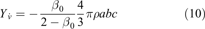
Finally, the final damping parameter is a diagonal matrix as follows

$D=\text{diag}\left[\begin{array}{c}{d}_1,d_2,d_3\end{array}\right]$

12

where elements are as follows, $d_1=10.77+1.26|u|,d_2=16.98+0.13|v|,d_3=9+0.2r$ .

Finally, based on simulated damping parameters, the nonlinear controller would be finished in the following section.

Controller design

In this section, based on the double integrator system, a Lyapunov directed controller was built up firstly which is similar with the model in the study by Yu, ³⁴ as shown in Figure 6. In addition, the integrator system was based on the ship’s path, orientation, and velocity errors, respectively. The objective of the controller is to drive a marine vessel following design path ${\text{p}}_d$ . According to the boat dynamic equations (3) and (4), a ship is an autonomous model which only consists of a propeller ${\tau }_u$ as ${[{\tau }_u\mathrm{,0,0}]}^{\text{T}}$ , that cannot fully control the ship’s movement. Therefore, the final backstepping control law only consists of propeller ${\tau }_u$ and rudder ${\tau }_r$ force.

Figure 6.

Boat control loop.

Backstepping for position and velocity error

At first, position error ${\mathbf{z}}_p\in {ℝ}^2$ was defined in initial frame $\left\{I\right\}$ and velocity error ${\mathbf{z}}_v\in {ℝ}^2$ was defined in body-fixed frame $\left\{B\right\}$

${\mathbf{z}}_{\mathbf{p}}=\mathbf{p}-{\mathbf{p}}_d$

13

${\mathbf{z}}_{\mathbf{v}}=R(\psi )\mathbf{v}-{\dot{\mathbf{p}}}_d$

14

According to ship kinematics and dynamic equations (1) to (4), the time derivative of error ${\mathbf{z}}_p$ and ${\mathbf{z}}_v$ are

${\dot{\mathbf{z}}}_p={\mathbf{z}}_v$

15

${\dot{\mathbf{z}}}_v=\ddot{\mathbf{p}}-{\ddot{\mathbf{p}}}_d$

16

where the acceleration $\ddot{\mathbf{p}}$ is denoted in equation (6).

The last function can be regarded as two closed-loop double integrator systems. Each system is driven by one of the vectors ${\dot{\mathbf{z}}}_v$ . In this case, the control law is in the following format, ${\mathbf{u}}^{\star }({\mathbf{z}}_p,{\mathbf{z}}_v)=[u(z_{p1},z_{v1}),u(z_{p2},z_{v2}),u(z_{p3},z_{v3}{)]}^{\text{T}}$ .

In addition, based on a transferred function in Young’s inequality, the position part was reformed as ${\mathbf{z}}_I={\displaystyle {\int }_0^t}{\mathbf{z}}_v(\tau )+\sigma ({\mathbf{z}}_p(\tau ))\text{d}\tau$ , where $\frac{\text{d}}{\text{d}\mathbf{t}}({\mathbf{z}}_I)=\sigma ({\mathbf{z}}_p)+{\mathbf{z}}_v$ .

The first tentative Lyapunov function

Based on saturated position error $\sigma ({\mathbf{z}}_p)$ and velocity error ${\mathbf{z}}_v$ , the first tentative Lyapunov function is

$\begin{array}{l}{V}_1=\varphi {({\mathbf{z}}_p)}^{\text{T}}\mathbf{1}+\frac{1}{2}{(\sigma ({\mathbf{z}}_p)+{\mathbf{z}}_v)}^{\text{T}}(\sigma ({\mathbf{z}}_p)+{\mathbf{z}}_v)\\ \hspace{1em}\hspace{1em}+{\displaystyle {\int }_0^{\parallel {\mathbf{z}}_I\parallel }}\sigma (\tau )\text{d}\tau +{\displaystyle {\int }_0^{\parallel \mathbf{b}\parallel }}{\sigma }^{-1}(\tau )\text{d}\tau -{\mathbf{b}}^{\text{T}}{\mathbf{z}}_I\end{array}$

17

where $\varphi ({\mathbf{z}}_p)={\displaystyle {\int }_0^{{\mathbf{z}}_p}}\sigma (\tau )\text{d}\tau$ . The time derivative of positive function $\varphi ({\mathbf{z}}_p)$ is $\sigma ({\mathbf{z}}_p){\mathbf{z}}_v$ . And the time derivative of $V_1$ is

$\begin{array}{l}{\dot{V}}_1=-W_1+{(\sigma ({\mathbf{z}}_p)+{\mathbf{z}}_v)}^{\text{T}}(\frac{1}{m}R\mathbf{t}-\frac{1}{m}D\dot{\mathbf{p}}-{\ddot{\mathbf{p}}}_d\\ \hspace{1em}\hspace{1em}-{\mathbf{u}}^{\star }+\sigma (\parallel {\mathbf{z}}_I\parallel )\frac{{\mathbf{z}}_I}{\parallel {\mathbf{z}}_I\parallel })\end{array}$

18

where $W_1({\mathbf{z}}_p,{\mathbf{z}}_v)$ is a positive definite function and $k_1$ is a control gain. The tentative input law is ${\mathbf{u}}^{\star }=-k_1(\sigma ({\mathbf{z}}_p)+{\mathbf{z}}_v)-\sigma ({\mathbf{z}}_p)-{\sigma }^{\prime }({\mathbf{z}}_p){\mathbf{z}}_v\mathrm{.}$

The thrust control law

Up to now, based on the first time derivative of Lyapunov function, the equilibrium of desired and actual acceleration is

$\frac{1}{m}R\mathbf{t}-\left(\frac{1}{m}D\dot{\mathbf{p}}+{\mathbf{u}}^{\star }+{\ddot{\mathbf{p}}}_d-\sigma (\parallel {\mathbf{z}}_I\parallel )\frac{{\mathbf{z}}_I}{\parallel {\mathbf{z}}_I\parallel }\right)$

19

where the rotation matrix is $R=[{\mathbf{r}}_1 {\mathbf{r}}_2 {\mathbf{r}}_3]$ and the control law was rewritten in direction format as follows

${\tau }_u={\tau }_{ud}{\mathbf{r}}_{1d}^{\text{T}}{\mathbf{r}}_1$

20

After substituting equation (20) into equation (19), the desired acceleration was replaced in direction format as

${\mathbf{a}}_d=\frac{1}{m}D\dot{\mathbf{p}}+{\mathbf{u}}^{\star }+\ddot{\mathbf{p}}-\sigma (\parallel {\mathbf{z}}_I\parallel )\frac{{\mathbf{z}}_I}{\parallel {\mathbf{z}}_I\parallel }$

21

In addition, the force equilibrium equation (19) includes actual ${\tau }_u$ and desired ${\tau }_{ud}$ values as follows

${\tau }_{ud}=m\Vert \frac{1}{m}D\dot{\mathbf{p}}+{\mathbf{u}}^{\star }+\ddot{\mathbf{p}}-\sigma (\parallel {\mathbf{z}}_I\parallel )\frac{{\mathbf{z}}_I}{\parallel {\mathbf{z}}_I\parallel }\Vert$

22

${\mathbf{r}}_{1d}=\frac{\frac{1}{m}D\dot{\mathbf{p}}+{\mathbf{u}}^{\star }+\ddot{\mathbf{p}}-\sigma (\parallel {\mathbf{z}}_I\parallel )\frac{{\mathbf{z}}_I}{\parallel {\mathbf{z}}_I\parallel }}{\Vert \frac{1}{m}D\dot{\mathbf{p}}+{\mathbf{u}}^{\star }+\ddot{\mathbf{p}}-\sigma (\parallel {\mathbf{z}}_I\parallel )\frac{{\mathbf{z}}_I}{\parallel {\mathbf{z}}_I\parallel }\Vert }$

23

As a consequence, based on actual and desired direction error ${\mathbf{r}}_1$ , ${\mathbf{r}}_{1d}$ , the first tentative Lyapunov function was rewritten as follows

${\dot{V}}_1=-W_1+\frac{{\tau }_{ud}}{m}{(\sigma ({\mathbf{z}}_p)+{\mathbf{z}}_v)}^{\text{T}}S{({\mathbf{r}}_1)}^2{\mathbf{r}}_{1d}$

24

In the following section, the calculations will focus on the next stage, direction error.

Backstepping for direction error

Firstly, the direction and orientation angle errors are

${\mathbf{z}}_d={\mathbf{r}}_1-{\mathbf{r}}_{1d}$

25

$\text{cos}{\mathbf{z}}_{\theta }=1-\frac{1}{2}{\mathbf{z}}_d^{\text{T}}{\mathbf{z}}_d={\mathbf{r}}_1^{\text{T}}{\mathbf{r}}_{1d}$

26

In addition, the second tentative Lyapunov function was extended with angular error as follows

$\begin{array}{c}{V}_2=V_1+\frac{1}{2k_2}{\mathbf{z}}_d^{\text{T}}{\mathbf{z}}_d+\frac{1}{2k_{b1}}{\tilde{\mathbf{b}}}_1^{\text{T}}{\tilde{\mathbf{b}}}_1\\ =V_1+\frac{1}{k_2}(1-\text{cos}{\mathbf{z}}_{\theta })+\frac{1}{2k_{b1}}{\tilde{\mathbf{b}}}_1^{\text{T}}{\tilde{\mathbf{b}}}_1\end{array}$

27

Finally, the time derivative of second tentative Lyapunov function is

$\begin{array}{l}{\dot{V}}_2=-W_2+(\frac{1}{k_2}{\mathbf{r}}_{1d}^{\text{T}}S({\mathbf{r}}_1)S({\mathbf{r}}_{1d})\frac{\partial {\dot{\mathbf{r}}}_{1d}}{\partial \text{b}}-\frac{1}{k_{b1}}{\dot{\widehat{\mathbf{b}}}}_1^{\text{T}}){\tilde{\mathbf{b}}}_1\\ \hspace{1em}+{\mathbf{r}}_{1d}^{\text{T}}RS({\mathbf{e}}_1)(S({\mathbf{e}}_1)R^{\text{T}}(\frac{{\tau }_{ud}}{m}(\sigma ({\mathbf{z}}_p)+{\mathbf{z}}_v)-k_3{\mathbf{r}}_{1d})\\ \hspace{1em}+\frac{1}{k_2}(\mathit{\omega }-R^{\text{T}}S({\mathbf{r}}_{1d}){\widehat{\dot{\mathbf{r}}}}_{1d}))\end{array}$

28

where $W_2=W_1+k_3{{\displaystyle \text{sin}}}^2{z}_{\theta }$ is a positive semi-definite function.

Backstepping for angular velocity

Angular velocity error

The second time derivative of Lyapunov function equation (28) relates to angular velocity $\mathit{\omega }$ . The angular velocity error is as follows

$\begin{array}{l}{\mathbf{z}}_{\mathit{\omega }}=S({\mathbf{e}}_1)R^{\text{T}}(\frac{{\tau }_{ud}}{m}(\sigma ({\text{z}}_p)+z_v)-k_3{\mathbf{r}}_{1d})\\ \hspace{1em}\hspace{1em}+\frac{1}{k_2}(\mathit{\omega }-R^{\text{T}}S({\mathbf{r}}_{1d}){\widehat{\dot{\mathbf{r}}}}_{1d})\end{array}$

29

Final Lyapunov function

The final Lyapunov function is a relay on angular acceleration error as follows

$V=V_2+\frac{1}{2}{\mathbf{z}}_{\mathit{\omega }}^{\text{T}}{\mathbf{z}}_{\mathit{\omega }}$

30

Time derivative of the final Lyapunov function is

$\begin{array}{l}\dot{V}=-W_3++{\mathbf{z}}_{\mathit{\omega }}^{\text{T}}(-S({\mathbf{e}}_1)R^{\text{T}}{\mathbf{r}}_{1d}+\frac{1}{k_2}\dot{\mathit{\omega }}+\widehat{\mathbf{h}}+k_4{\mathbf{z}}_{\mathit{\omega }})\\ \hspace{1em}\hspace{1em}+({\mathbf{z}}_{\mathit{\omega }}^{\text{T}}\frac{\partial \mathbf{h}}{\partial \mathbf{b}}-\frac{1}{k_2}{\mathbf{r}}_{1d}^{\text{T}}S({\mathbf{r}}_1)S({\mathbf{r}}_{1d})\frac{\partial {\dot{\mathbf{r}}}_{1d}}{\partial \mathbf{b}}-\frac{1}{k_{b1}}{\dot{\widehat{\mathbf{b}}}}_1^{\text{T}}){\tilde{\mathbf{b}}}_1\end{array}$

31

where $W_3=W_2+k_4{\mathbf{z}}_{\mathit{\omega }}^{\text{T}}{\text{z}}_{\mathit{\omega }}$ .

The symbol $\widehat{\mathbf{h}}$ represents estimation disturbance as

$\begin{array}{l}\mathbf{h}=\frac{\text{d}}{\text{d}t}\{S({\mathbf{e}}_1)R^{\text{T}}(\frac{{\tau }_{ud}}{m}(\sigma ({\mathbf{z}}_p)+{\mathbf{z}}_v)-k_3{\mathbf{r}}_{1d})\\ \hspace{1em}\hspace{1em}-\frac{1}{k_2}{R}^{\text{T}}S({\mathbf{r}}_{1d}){\widehat{\dot{\mathbf{r}}}}_{1d}\}\end{array}$

32

In order to achieve global trajectory tracking and guarantee $\dot{V}$ being negative semi-definite, the final control law relative to torque is

${\tau }_{rd}=(I_{zz}-N_{\dot{r}}){\mathbf{e}}_3{\dot{\mathit{\omega }}}_d+N_{r}r+N_{|r|r}|r|r$

33

where the time derivative of desired angular velocity is

${\dot{\mathit{\omega }}}_d=-k_2(-S({\mathbf{e}}_1)R^{\text{T}}{\mathbf{r}}_{1d}+\widehat{\mathbf{h}}+k_4{\mathbf{z}}_{\mathit{\omega }})$

34

Up to this step, all of the Lyaounov function calculations were finished. In following section, the disturbance estimation update law will be introduced in detail.

Estimation update law with smooth projection operator

The estimate update law is

$\begin{array}{c}\dot{\widehat{\mathbf{b}}}=k_b\mathbf{Proj}(\xi ,\widehat{\mathbf{b}})\\ =k_b(\xi -\frac{{\eta }_1{\eta }_2}{2({\epsilon }^2+2\epsilon B{)}^{n+1}{B}^2}\widehat{\mathbf{b}})\end{array}$

35

with the following functions

$\xi ={\left({\mathbf{z}}_{\mathit{\omega }}^{\text{T}}\frac{\partial \mathbf{h}}{\partial \mathbf{b}}-\frac{1}{k_2}{\mathbf{r}}_{1d}^{\text{T}}S({\mathbf{r}}_1)S({\mathbf{r}}_{1d})\frac{\partial {\dot{\mathbf{r}}}_{1d}}{\partial \mathbf{b}}\right)}^{\text{T}}$

36

${\eta }_1=\{\begin{array}{ll}{({\widehat{\mathbf{b}}}^{\text{T}}\widehat{\mathbf{b}}-B^2)}^{n+1}\hfill & \text{if} ({\widehat{\mathbf{b}}}^{\text{T}}\widehat{\mathbf{b}}-B^2)>0\hfill \\ 0\hfill & \text{otherwise}\hfill \end{array}$

37

${\eta }_2={\widehat{\mathbf{b}}}^{\text{T}}\xi -\sqrt{{({\widehat{\mathbf{b}}}^{\text{T}}\xi )}^2+{\kappa }^2},$

38

where $\epsilon >0$ and $\kappa >0$ are arbitrary parameters and $B>0$ is the bound on the norm of the unknown disturbance. The smooth projection operator is taken from Cai et al. ²⁵ and has the following properties:

$\text{P}1-\parallel \widehat{\mathbf{b}}(t)\parallel \le B+\epsilon ,\forall t\ge 0;$

$\text{P}2-{\tilde{\mathbf{b}}}^{\text{T}}\mathbf{Proj}(\xi ,\widehat{\mathbf{b}})\ge {\tilde{\mathbf{b}}}^T\xi ;$

$\text{P}3-\parallel \mathbf{Proj}(\xi ,\widehat{\mathbf{b}})\parallel \le \parallel \xi \parallel {(1+(\frac{B+\epsilon }{B}))}^2+\frac{B+\epsilon }{2B^2}\kappa ;\hspace{0.17em}\text{and}$

$\text{P}4-\mathbf{Proj}(\xi ,\widehat{\mathbf{b}})$ is ${ℂ}^n$ .

Based on the estimation law, the final Lyapunov function was established.

Control law conclusion

Up to now, all the backstepping calculations have been finished. The final conclusion generated that the time derivative of Lyapunov function $\dot{V}$ is negative semi-definite based on the remaining driving ${\tau }_{\mathbf{u}}$ , ${\tau }_{\mathbf{r}}$ and the disturbance estimation law equation (35). In the following parameter, a Barbalat’s lemma will prove the conclusion as follows:

If $f(t)$ has a finite limit as $t\to \infty$ and if $\dot{f}$ is uniformly continuous (or $\ddot{f}$ is bounded), then $\dot{f}(t)\to 0$ as $t\to \infty$ .

Proof

Let the boat kinematics and dynamics be questions equations (1) to (4) respectively. Let ${\mathbf{p}}_d\in {ℂ}^3$ be the design position and $\psi \in ℂ$ be orientation. The closed-loop system forms a controller law about force ${\tau }_u$ and torque ${\tau }_r$

${\tau }_u={\tau }_{ud}{\mathbf{r}}_{1d}^{\text{T}}{\mathbf{r}}_1$

39

${\tau }_r=(I_{\mathbf{z}\mathbf{z}}-N_{\dot{r}}){\mathbf{e}}_3{\dot{\mathit{\omega }}}_d+N_{r}r+N_{|r|r}|r|r$

40

The controller achieves trajectory tracking by guaranteeing the errors $({\mathbf{z}}_p,{\mathbf{z}}_v,z_{\theta },{\mathbf{z}}_{\mathit{\omega }})$ converging to uniformly asymptotically stable equilibrium $(0 0 0 0)$ or $(0 0 \pi 0)$ for any properly initial condition.

If any actual boats satisfy $I_{\mathbf{z}\mathbf{z}}\ne N_{\dot{r}}$ , the system positive definite Lyapunov function is

$\begin{array}{c}V=\varphi {({\mathbf{z}}_p)}^{\text{T}}\text{1}+\frac{1}{2}{(\sigma ({\mathbf{z}}_p)+{\mathbf{z}}_v)}^{\text{T}}(\sigma ({\mathbf{z}}_p)+{\mathbf{z}}_v)\\ +{\displaystyle {\int }_0^{\parallel {\mathbf{z}}_I\parallel }}\sigma (\tau )\text{d}\tau +{\displaystyle {\int }_0^{\parallel \mathbf{b}\parallel }}{\sigma }^{-1}(\tau )\text{d}\tau -{\mathbf{b}}^{\text{T}}{\mathbf{z}}_I\\ +\frac{1}{2k_2}{\mathbf{z}}_d^{\text{T}}{\mathbf{z}}_d+\frac{1}{2k_{b1}}{\tilde{\mathbf{b}}}_1^{\text{T}}{\tilde{\mathbf{b}}}_1+\frac{1}{2}{\mathbf{z}}_{\mathit{\omega }}^{\text{T}}{\mathbf{z}}_{\mathit{\omega }}\end{array}$

41

and its time derivative computed as

$\begin{array}{l}\dot{V}=-\sigma {({\mathbf{z}}_p)}^{\text{T}}\sigma ({\mathbf{z}}_p)-k_1{(\sigma ({\mathbf{z}}_p)+{\mathbf{z}}_v)}^{\text{T}}(\sigma ({\mathbf{z}}_p)+{\mathbf{z}}_v)\\ \hspace{1em}\hspace{0.17em}\hspace{0.17em}-k_3{{\displaystyle \text{sin}}}^2{z}_{\theta }-k_4{\mathbf{z}}_{\mathit{\omega }}^{\text{T}}{\mathbf{z}}_{\mathit{\omega }}\end{array}$

42

which is a semi-negative definite function.

Finally, based on the positive definite V with respect to $({\mathbf{z}}_p,{\mathbf{z}}_v,z_{\theta },{\mathbf{z}}_{\mathit{\omega }})$ and $\tilde{\mathbf{b}}$ , we conclude that V has a lower bound. Regarding the negative semi-definite function $\dot{V}$ under ideal condition, we conclude that the states $({\mathbf{z}}_p,{\mathbf{z}}_v,z_{\theta },{\mathbf{z}}_{\mathit{\omega }})$ converge to equilibrium set $(0,0,0,0),(0,0,\pi \mathrm{,0})$ . We have thus that the $\ddot{V}$ is bounded and consequently, $\dot{V}$ is uniformly continuous. Therefore, we can apply Barbalat’s Lemma to prove $\dot{V}$ convergence to equilibrium.

Simulation result

Trajectory tracking performance

In order to simulate the proposed controller, the boat prediction route was set as a circle, with radius $\text{30}\hspace{0.17em}\text{m}$ , centered at position $[0,-30,0]$ in the initial frame. The desired cruising velocity in the body-fixed frame was ${\text{v}}_d=[u_d{\mathrm{,0,0}]}^{\text{T}}$ and $u_d=\text{1.2}\hspace{0.17em}\text{m/s}$ . The boat’s initial position was defined as ${[-\text{15} -\text{10} \text{0}]}^{\text{T}}$ (m). Finally, the control law coefficients were $k_1=3.2,k_2=7,k_3=6,k_4=40,k_{\mathbf{b}1}=0.5$ and the constant disturbance vector was ${[1.2 1.5 0]}^{\text{T}}$ with force unit $\text{N}$ .

Tracking performance with disturbance

Finally, the boat’s tracking performance with disturbance was presented in Figure 7. The boat followed a circular path with small position errors after a short time for adjustment. The adjustment time depended on disturbance, water fluid hydrodynamic and the ship’s shape characteristics.

Figure 7.

Boat reference and actual path with disturbance.

Error performance

As Figure 8 shows, the position and velocity errors ${\mathbf{z}}_p,{\mathbf{z}}_v$ were similar to the performance without disturbance. In the beginning, orientation and direction errors ${\mathbf{z}}_d$ and ${\mathbf{z}}_{\theta }$ were vibrating a little. Angular velocity error ${\mathbf{z}}_{\mathit{\omega }}$ remained near to zero. As time passed, all of the errors converged to zero without sudden shock. This means that the controller was working wonderfully under the ocean’s current disturbance.

Figure 8.

The error simulation with disturbance.

Disturbance estimation

The unknown current disturbance was estimated by a smooth projection operator. As in Figure 9, the actual disturbance was assumed to be ${[1.2 1.5 0]}^{\text{T}}$ . The estimation approached actual value. As in Figure 8, the disturbance estimation worked normally and ultimately achieved target value.

Figure 9.

The boat disturbance estimation results.

Conclusion

The article introduces the methodology of CFD simulation result certificated by USV trajectory tracking control system. The trajectory tracking performance works with unknown disturbance. As an actual condition, a boat’s hydrodynamic parameters are about nonlinear damping and centripetal force. In general, the tracking controller is based on Lyapunov direct method and backstepping techniques. The final simulation results denotes that the trajectory tracking errors converge to a bounded equilibrium. This means that the controller works wonderfully under ocean current disturbance. In addition, it proves that the CFD simulation result is proper for boat hydrodynamics. As an innovation point, the simulation method will be of use to some small laboratory without large experiment equipment. CFD technology can solve the problems caused by equipment or limited funds. However, there are still disadvantages. The actual Q-boat experiments have not been finished because of changes in research schedule. This means that there is lack of actual data to compare with the estimation result. In future, the Q-boat will upgrade with ROS and accurate GPS navigation equipment. Some related experiements will take into consideration such things as multi-boat formation control, boat-submarine leader following control and sea-bed communication control with time delay.