Sage Journals: Discover world-class research

Abstract

A robust control algorithm for tracking a wheeled mobile robot navigating in a pre-planned path while passing through the road’s roundabout environment is presented in this article. The proposed control algorithm is derived from both the kinematic and dynamic modelling of a non-holonomic wheeled mobile robot that is driven by a differential drive system. The road’s roundabout is represented in a grid map and the path of the mobile robot is determined using a novel approach, the so-called laser simulator technique within the roundabout environment according to the respective road rules. The main control scheme is experimented in both simulation and experimental study using the resolved-acceleration control and active force control strategy to enable the robot to strictly follow the predefined path in the presence of disturbances. A fusion of the resolved-acceleration control–active force control controller with Kalman Filter has been used empirically in real time to control the wheeled mobile robot in the road’s roundabout setting with the specific purpose of eliminating the noises. Both the simulation and the experimental results show the capability of the proposed controller to track the robot in the predefined path robustly and cancel the effect of the disturbances.

Keywords

Non-holonomic wheeled mobile robot Lagrange–Euler equation resolved-acceleration control laser simulator active force control strategy fuzzy logic

Introduction

Nowadays, mobile robots are a common feature in many applications that involve hazardous, complex, high accurate or heavy-duty tasks in various fields such as aerospace, underwater, military, medicine, inspection and mining. Usually, the robot is expected to navigate autonomously in either structured or non-structured environments, with both needing a robust control scheme to determine its path within the terrain and avoid obstacles.

In some conditions, such as road environments, it is imperative to control the robot robustly in the planned path to avoid crashing into cars or people. Different methods and techniques have been investigated to solve the problems of mobile robot motion control; some of them depend solely on the kinematics of the mobile robot; others on the dynamics only or a combination of both.

A wheeled mobile robot (WMR) control system with a dynamics feed-forward compensation is used for servo control of an autonomous mobile robot adaptive to variations of movements using the recursive least square method for online parameters estimator.¹

Fuzzy logic (FL) controller with a reference speed derived from the curvature of the trajectory that is detected by camera and image processing software is used to control the mobile robot.² FL controller is preferred due to some favourable properties such as having excellent potentials in handling non-linear system and producing a fast dynamic response, which often resulted in an accurate dynamic model of system.³ In another study, FL controller is implemented for controlling a WMR motion in unstructured environments with obstacles and slopes.⁴ An adaptive method using a kinematic and torque controller based on FL reasoning is used for intelligent control of an autonomous mobile robot.⁵

Neural network (NN) controller is utilized for controlling the motion of a mobile robot through a three-layered architecture to define the relationship between the linear velocities and the error positions of the mobile robot.⁶

A cross-coupling method is used in a differential drive system for controlling the velocity of both motors, in which the control loop of each motor uses the position error of the other one.⁷ A stable tracking control system⁸ is used for adjusting the linear and rotational velocities of mobile robot using a Lyapunov function, which depends on linearizing the kinematic model with feedback control. An approach based on feedback sliding mode control is used for stabilizing of non-holonomic mobile robot.⁹ In another work, the sliding-mode control method is utilized for stabilization and tracking of non-holonomic mobile robots using kinematics in polar coordinates.¹⁰ The back-stepping control approach with the integration of kinematic and torque controllers has been implemented for controlling the non-holonomic mobile robots.¹¹ An adaptive extension of the back-stepping controller is used for non-holonomic mobile robot control, in which, the tracking controller for the dynamics of the system can be investigated by applying the adaptive back-stepping algorithm with the existence of an adaptive controller based on the kinematics.¹²

A tracking control system with time-varying feedback based on back-stepping is employed for the tracking control of a mobile robot.¹³ In this method, a combination of the kinematic and simplified dynamic model in a 2-degree-of-freedom mobile robot is used to find the local and global tracking parameters. A non-linear modelling and control of the mobile robot has been implemented using an adaptive method with NN to improve the associative searching element.¹⁴ This controller is derived from the Lyapunov stability theory and can guarantee tracking performance and stability with small errors.

A novel robust control approach-based voltage control strategy has been developed by Fateh and Arab.¹⁵ In this work, the robot dynamics and state space model of the electrical voltage are used to build a complete control model for driving the non-holonomic WMR. In another development, active force control (AFC) strategy has been widely implemented for controlling the dynamics of a mobile manipulator system, which resulted in a robust control scheme especially with the existence of disturbances.^16

–19 The method depends on the measurements of the applied torque and acceleration plus a good approximation of the estimated inertia matrix to estimate the force feedback of the control system.^20
–22

Luy has proposed an optimal algorithm to solve the problem of unknown or uncalibrated disturbances for nonholonomic mobile multirobot (NMMR) using an omnidirectional vision sensor.²³ The optimal tracking using both the system kinematics and dynamics has been initially transformed into equivalent optimal control for disturbance rejection. The differential game theory is integrated into the Hamilton–Jacobi–Isaac equations to stabilize the closed-loop system. Another adaptive optimal algorithm has been proposed for solving the dynamic equations for a WMR incorporating an omnidirectional vision system.²⁴

The controller depends on the integration of its kinematics and dynamics while passing on the feedback of the dynamic system as tracking errors. A robust adaptive dynamic programming algorithm control approach based on NN has been used to solve the problem of a two player with zero-sum game, which in turn help to estimate the solution of Hamilton–Jacobi–Isaacs equation without any prior knowledge of the dynamic system.

A kinematic and dynamic control system based on reinforcement learning has been employed for controlling a WMR.²⁵ Using a single NN layer, a tuning law with Hamilton–Jacobi–Isaacs equation is adopted to estimate the optimal tracking path (H_∞ ) and guarantee the stability of the control system in real time.

A computed torque controller combined with a novel model state observer control is used for path tracking control of a robotic manipulator.²⁶ To get a precise dynamic model and eliminate the effect of noises, model-assisted extended state observer has been used to eliminate the structured/unstructured noises and enhance the computed torque control performance. The observer is able to estimate the uncertainties in the dynamic system and enables to compensate the disturbances online that subsequently leads to a robust trajectory tracking control of the robotic manipulator with high disturbance rejection capability. Another trajectory tracking robotic system using computed torque control scheme with dynamic modelling is used to control a WMR manipulator in the task space.²⁷ Using a well-known model of a computed torque control, it has been proved that the stability of the system is guaranteed and the convergence of tracking errors has been reached.

In this article, a new robust controller called Kalman Filter (KF)-resolved-acceleration control (RAC)-AFC has been introduced to control a mobile robot in a roundabout environment. Actually, the control of a mobile robot in a relatively complex environment such as a road roundabout setting during a path execution is still regarded as a challenging problem in mobile robot research, because it needs to maintain the tracking errors at near-zero level.²⁸ Thus, there is a need for a robust controller to guarantee such small tracking errors along the movement. AFC has been used widely for controlling the dynamics of the robot and rejecting the disturbances, but it trends to an overshoot of tracking errors at the beginning of movement and when there is a sudden change in the path as shown in Figure 5(d) and (e) and Figure 7(b) and (c). The RAC kinematic controller on other hand, when combined with AFC, can enhance the performance of controller at the beginning and sudden changes of the robot movement as shown in Figure 5(d) and (e) and Figure 7(b) and (c). However, in the real-time control system, the sensors’ measurements used in the feedbacks of WMR kinematics and dynamics are subjected to uncertainties and noises, which have to be eliminated using KF in the proposed controller. Therefore, the proposed control scheme consists of three feedback loops, that is, the external and internal loops. The former consists of two loops and is utilized for controlling the kinematic parameters using the RAC and the latter is for controlling the dynamic parameters and compensating the disturbances through the AFC controller. In other words, the contribution of this article can be summarized as follows:

The movement of the robot in a road roundabout environment with its entrances and exits are investigated and controlled well in real-time as one of the first works involving such surroundings and settings. Because of some limitations related to safety and accuracy issues such as inability to clearly identify or recognize a roundabout in some locations using GPS, the signal losses in GPS and problems in interpreting the sudden changes in the road environment, it may cause unwarranted harm and damage to pedestrians and road curbs. Thus, it is often necessary to use on-board sensors with a robust control system for real-time detection and decision-making in a roundabout environment.

A new control strategy that integrates the RAC and AFC approaches employing the use of FL and KF in real time is applied to robustly navigate the path in the roundabout environment as one of the pioneering works that involves the integration of such algorithms. Since the roundabout area is a relatively challenging path to navigate considering various factors and uncertainties, it demands a high degree of tracking accuracy from the control system. By incorporating the RAC strategy for controlling the kinematics of robot and AFC for the dynamics, all comprising three control loops, a zero tracking error is a strong possibility. Since, most of the sensors contain some level of noises, KF has been included in the control system to eliminate these noises and uncertainties in the reference trajectory of the control system prior to reaching the control loops. The stability of the new controller scheme has been proved using Lyapunov function to find its convergence and boundedness.

Modelling the non-holonomic WMR

The robot is supposed to move on a flat plane where the motion can be described in x and y directions using three wheels: two differential wheels and castor as shown in Figure 1. The movement is generated by two motors, which are switching the right and left wheels through the angular velocities, ${\dot{θ}}_{r}$ and ${\dot{θ}}_{l}$ , respectively. The heading direction determines the rotation of mobile robot in counter clockwise as shown in Figure 1. The robot motion can be described in two coordinate systems, namely the global coordinate system (X, Y, ϕ) axis and local coordinate system (W, V) as shown in Figure 1. In the global coordinate system, the motion can be obtained in three axes, q = [x, y, ϕ]^T as in Figure 1, whereas the local coordinate system has only two axes, w and v. The centre of the non-holonomic mobile robot has some constraints in its movements, since the wheels are assumed to move with pure rolling and without slipping on the ground, and it can move only in the normal axis of the driving wheels (no sideway movements). These constraints can be written as in equation (1)

A (q) \dot{q} = [\begin{matrix} - sin (φ) & cos(φ) & - d & 0 & 0 \\ cos(φ) & sin(φ) & - b & - r & 0 \\ cos(φ) & sin(φ) & b & - r & 0 \end{matrix}] [\begin{matrix} \dot{x} \\ \dot{y} \\ \dot{φ} \\ {\dot{θ}}_{r} \\ {\dot{θ}}_{l} \end{matrix}] = 0

Figure 1.

Mobile robot dimensions with global and local coordinate system.

In equation (1) and Figure 1, L represents the length of the robot; 2b is the distance between the two wheels; r is the radius of the driving wheels (both wheels are with same radius); d is the displacement between the driving wheel shaft and the mass centre c of the mobile robot.

Mobile robot kinematics

The mobile robot is driven by two differential wheels with a rear castor wheel as shown in Figure 1. The linear right and left wheels velocities are expressed as

V_{r} = r {\dot{θ}}_{r}; V_{l} = r \dot{θ}

where ${\dot{θ}}_{r}$ and ${\dot{θ}}_{l}$ are the angular velocities in the right and left wheels, respectively.

The average linear velocity of the WMR is

V = \frac{V_{r} + V_{l}}{2} = \frac{r \overset{​}{{\dot{θ}}_{r} + r {\dot{θ}}_{l}}}{2} = [\frac{r}{2} \frac{r}{2}] [\begin{matrix} {\dot{θ}}_{r} \\ {\dot{θ}}_{l} \end{matrix}]

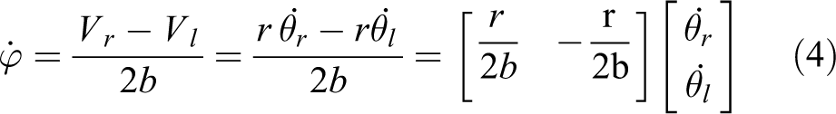
The heading angular velocity of the WMR is then equal to the difference between the angular velocities of the right and left wheels, which is

\dot{φ} = \frac{V_{r} - V_{l}}{2 b} = \frac{r \overset{​}{{\dot{θ}}_{r} - r {\dot{θ}}_{l}}}{2 b} = [\begin{matrix} \frac{r}{2 b} & - \frac{r}{2b} \end{matrix}] [\begin{matrix} {\dot{θ}}_{r} \\ {\dot{θ}}_{l} \end{matrix}]

The velocity of the robot in a global coordinate system can be described relatively to the local coordinate system as in equation (5)

[\begin{matrix} \dot{x} \\ \dot{y} \\ \dot{φ} \end{matrix}] = [\begin{matrix} cos(φ) & - d sin(φ) \\ sin(φ) & d cos(φ) \\ 0 & 1 \end{matrix}] [\begin{matrix} V \\ \dot{φ} \end{matrix}]

By substituting equations (3) and (4) into equation (5), the velocity of the mobile robot can be written in terms of the angular velocities, $\dot{θ_{r}}$ and $\overset{}{θ_{l}}$ as in equation (6).

[\begin{matrix} \dot{x} \\ \dot{y} \\ \dot{φ} \end{matrix}] = [\begin{matrix} \frac{r}{2} cos (φ) - \frac{d r}{2 b} sin (φ) & \frac{r}{2} cos (φ) + \frac{d r}{2 b} sin (φ) \\ \frac{r}{2} sin (φ) + \frac{d r}{2 b} cos (φ) & \frac{r}{2} sin (φ) - \frac{d r}{2 b} cos (φ) \\ \frac{r}{2 b} & - \frac{r}{2 b} \end{matrix}] [\begin{matrix} {\dot{θ}}_{r} \\ {\dot{θ}}_{l} \end{matrix}]

The current position of the robot is thus given by equation (7)

[\begin{matrix} x_{n} \\ y_{n} \\ φ_{n} \end{matrix}] = [\begin{matrix} 1 & 0 & 0 \\ 0 & 1 & 0 \\ 0 & 0 & 1 \end{matrix}] [\begin{matrix} x_{n - 1} \\ y_{n - 1} \\ φ_{n - 1} \end{matrix}] + \nabla T [\begin{matrix} \frac{r}{2} cos (φ) - \frac{d r}{2 b} sin (φ) & \frac{r}{2} cos (φ) + \frac{d r}{2 b} sin (φ) \\ \frac{r}{2} sin (φ) + \frac{d r}{2 b} cos (φ) & \frac{r}{2} sin (φ) - \frac{d r}{2 b} cos (φ) \\ \frac{r}{2 b} & - \frac{r}{2 b} \end{matrix}] [\begin{matrix} {\dot{θ}}_{r} \\ {\dot{θ}}_{l} \end{matrix}]

where X_n, Y_n, φ_n are the current positions of the WMR, X_n−1, Y_n−1, φ_n−1 are the previous positions of the WMR and ∇T is the sampling time of the measurements.

Mobile robot dynamics

The dynamic equations of the mobile robot can be determined using Newton’s law or Euler–Lagrange formulation. In this research, the Lagrange equation was used to derive the dynamic equations of the robot as in equation (8)

\frac{\partial}{d t} \frac{\partial k}{\partial q_{i}} - \frac{\partial k}{\partial q_{i}} = τ_{i} - A^{T} (q) λ

where K is the summation of the kinetic and potential energies.

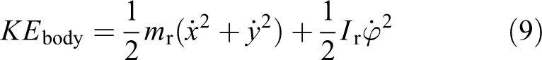
The potential energy in this project can be neglected since the height of robot from the ground very low. q is the coordinate system, τ is the exerted torque on the robot, A ^T(q) is the constraints of robot movement. The kinetic energy of the body of the WMR can be written as in equation (9)

K E_{body} = \frac{1}{2} m_{r} ({\dot{x}}^{2} + {\dot{y}}^{2}) + \frac{1}{2} I_{r} {\dot{φ}}^{2}

The kinetic energy of the right wheel can be written as in equation (10).

\begin{matrix} K E_{r w} = \frac{1}{2} m_{w} {(\dot{x} + b \dot{φ} cos (φ) + d \dot{φ} sin (φ))}^{2} \\ + \frac{1}{2} m_{w} {(\dot{y} + b \overset{​}{\dot{φ} sin (φ) -} d \dot{φ} cos (φ))}^{2} + \frac{1}{2} I_{W} {\dot{φ}}^{2} + \frac{1}{2} I_{W} {\dot{θ}}_{r}^{2} \end{matrix}

And the kinetic energy of the left wheel can be written as in equation (11).

\begin{matrix} K E_{l w} = \frac{1}{2} m_{w} {(\dot{x} - b \dot{φ} cos (φ) + d \dot{φ} sin (φ))}^{2} \\ + \frac{1}{2} m_{w} {(\dot{y} - b \overset{​}{\dot{φ} sin (φ) -} d \dot{φ} cos (φ))}^{2} + \frac{1}{2} I_{W} {\dot{φ}}^{2} + \frac{1}{2} I_{W} {\dot{θ}}_{l}^{2} \end{matrix}

By deriving the kinetic energy of the body, left and right wheels as in equations (9) to (11), the Lagrange equation can be written as in equation (12)

M (q) \ddot{q} + V (q, \dot{q}) = τ - A^{T} (q) λ

where

\begin{array}{l} M (q) = [\begin{matrix} m & 0 & 2 m_{ω} d sin (φ) & 0 & 0 \\ 0 & m & - 2 m_{ω} d cos (φ) & 0 & 0 \\ 2 m_{ω} d sin (φ) & - 2 m_{ω} d sin (φ) & I & 0 & 0 \\ 0 & 0 & 0 & I_{ω} & 0 \\ 0 & 0 & 0 & 0 & I_{ω} \end{matrix}] \\ V (q, \dot{q}) = [\begin{array}{l} 2 m_{ω} d {\dot{φ}}^{2} sin (φ) \\ 2 m_{ω} d {\dot{φ}}^{2} cos (φ) \\ 0 \\ 0 \\ 0 \end{array}] \\ λ = [\begin{array}{l} λ_{1} \\ λ_{2} \\ λ_{3} \end{array}] τ = [\begin{matrix} 0 \\ 0 \\ 0 \\ τ_{r} \\ τ_{l} \end{matrix}] \end{array}

where A ^T(q) is the transpose of the constraints equation A(q) as in equation (1). The other parameters are defined as follows:

m: total mass of WMR = m _c + 2 m _w; m _c: the mass of the platform without the driving wheels and DC motors; m _w: the mass of the driving wheels and the DC motors; I: total moment of inertia of mobile robot.

I = I_{c} + 2 m_{ω} (d^{2} + b^{2}) + 2 I_{m}

I_c : the moment of inertia of the body of robot without the driving wheels and the motors about axis passed through P; I _ω: the moment of inertia of each wheel and the motor rotor about the wheel axis; I _m: the moment of inertia of each wheel and the motor rotor about the wheel diameter; τ _r: the torque exerted on wheel axis by right motor; τ _l: the torque exerted on wheel axis by left motor and; λ: the Lagrange multiplier coeficient.

Controller design

The path of the mobile robot is controlled using resolved-acceleration control (RAC), AFC and RAC-AFC-KF strategy. In RAC-AFC-KF, there are two feedback loops in the control scheme, the so-called external and internal loop as in Figure 2; the external loop is used for controlling the kinematic parameters by the RAC, and the internal loop is used for controlling the dynamics of robot through the AFC controller. KF is used to eliminate the noises and uncertainties from the measurements.

Figure 2.

A schematic of the RAC-AFC-KF controller. RAC: resolved-acceleration control; AFC: active force control; KF: Kalman Filter.

RAC control strategy

This controller is working based on minimizing of the position and orientation errors to zero, which needs to apply suitable torque or forces to the system using the following equation

\frac{\partial^{2}}{\partial t^{2}} (x_{ref} - x_{act}) + K_{1} \frac{\partial}{\partial t} (x_{ref} - x_{act}) + K_{2} (x_{ref} - x_{act}) = 0

where K₁, K₂ are scalar constants related to the input torque of the system. X _act and X _ref are the actual and reference trajectories, respectively.

AFC control strategy

AFC controller is the inner loop of the proposed controller, and it is mainly dependent on the angular acceleration feedbacks of the of wheel motors.

In the real-world environment, AFC controller can be described as the torque signal applied to actuators that drive the wheels based on the measured angular acceleration of the wheels via the sensors. The product of the measured acceleration with the estimated inertial matrix (IN) signal was compared with the applied torque (τ) as in equation (14). By estimating the inertia matrix using suitable technique, the controller can compensate effectively the effect of the disturbances. In simulation, the measurements are assumed to be ideal (perfect modelling). The equation that is used to estimate the disturbances can be written as in equation (14)

τ_{d}^{*} = τ - I N \ddot{θ}

where $τ_{d}^{*}$ is the estimated torque disturbance effected on the wheels. τ is the actuated torque that can be calculated in the case of a DC torque motor using the equation: τ = K _t I where K _t is the torque constant of the DC motor, I is the armature current and IN is the estimated inertia matrix, which has to be estimated well during the robot movement.

Estimation of inertial matrix

The estimation of the inertia matrix is necessary to compute the actual torque of the WMR from the disturbance torque obtained using equation (15) for the AFC control action. The moment of inertia must be appropriately estimated. As a rule of the thumb, the initial values of the elements in IN are assumed to be the values of M (q) computed by the dynamic model or lie within a suitable range¹⁸ as in equation (15)

0.4 M (q) < I N < 1.4 M (q)

There are many methods that can be used to calculate the inertia matrix during the robot movement such as crude approximation^14,16 and artificial intelligence (AI) approaches, e.g. NN,¹⁸ iterative learning,¹⁹ knowledge-based²¹ and FL.²² Since the inertia matrix typically has a known range as expressed in equation (16), it is sometimes preferred to use the FL controller. In addition, ϕ is the only variable in M(q) that is instrumental for the inertia matrix estimation. Thus, ϕ was chosen as the input set of the FL system while IN for both the right and the left wheels of the WMR were assigned as the outputs. As a result, we have only three variables as the input and output of the FL which can be adjusted. More variables will lead to complex fuzzy system while less sets leads to inaccurate FL modelling. The FL system then calculates the estimated IN necessary for the computation of the actual torque of the AFC controller for a given set of inputs. FL methodology passes through the following steps:

Fuzzification: In this process the crisp values is transformed into fuzzy values through finding the linguistic variables of the fuzzy set and determining the suitable membership function to arrange the relation between these variables. Thus, the mass matrix, M(q) in equation (12), can vary accordingly to the changes in sin (ϕ) and cos(ϕ), we chose ϕ as the input to FL, which was fuzzified into the following linguistic terms:

ϕ = [Very Low, Low, Medium, High, Very High]

Figure 3. shows the membership functions of the input and output sets.

Figure 3.

Fuzzy logic membership functions: (a) membership function of the fuzzy input set (ϕ); (b) membership function of the fuzzy output set (INL); (c) membership function of the fuzzy output set (INR).

The output of the FL is fuzzified into the following linguistic variables:

INR/INL = {Very Small, Small, Medium, Large, Very Large}

It was found after some trials that the triangular shapes of the membership functions are suitable for calculating the value of the inertia matrix.

Rule Interface: It is used to define the relationship between the crisp input and output through the linguistic expressions (if–then statements) based on two approaches, namely, Sugeno or Mamdani. In this simulation, the fuzzy interface system is using the Mamdani type as follows:

If (phi is M) then (INR is MR)&(INL is ML)

If (phi is VL) then (INR is VSR)&(INL is VLL)

If (phi is L) then (INR is SR)&(INL is LL)

If (phi is H) then (INR is LR)&(INL is SL)

If (phi is VH) then (INR is VLR)&(INL is VSL)

Defuzzification: All fuzzy outputs are aggregated using the centroid weighted method and the fuzzy output is transformed into a crisp output. In this simulation, the centroid method is used for defuzzification using equation (16)

x = \frac{\int μ_{i} (x) x d x}{μ_{i} (x) d x}

Stability analysis of RAC-AFC

According to the Lagrange equation, the torque of dynamic system is given by equation (12).

The dynamic system with the closed-loop feedback compensation as shown in Figure 2 can be calculated by equation (17)

M (q) ({\ddot{q}}_{d} + k_{d} {\dot{e}}_{q} + k_{p} e_{q}) + e_{τ} = τ

With equality of torque of robot as in equation (12) with the estimation torque using equation (17), one will get

M (q) \ddot{q} + V (q, \dot{q}) = M (q) ({\ddot{q}}_{d} + k_{d} {\dot{e}}_{q} + k_{p} e_{q}) + e_{τ}

By simplifying equation (18), one can get

{\ddot{e}}_{q} + k_{d} {\dot{e}}_{q} + k_{p} e_{q} = M {(q)}^{- 1} (V (q, \dot{q}) - e_{τ})

Lemma

Let V(t) is the Lyapunov function of the continuous-time control system. If V(t) is satisfying the differential inequality as in equation (20)

\dot{V} \leq - α V + γ (t)

where α is a positive constant. γ(t) is a function based on time which has positive values when t>0 and can achieve the condition $lim_{t \to \infty} γ (t) = C$ , this will guarantee that the closed loop will reach the global uniform ultimate boundedness for any value of t.

Theorem

The mobile robot control based on equation (7) with noises is considered. If ${\dot{e}}_{τ}$ is bounded, then the controller that was derived based on RAC and AFC, with equations (14) and (15), respectively, could guarantee to reach the global uniform ultimate boundedness of the closed-loop scheme with exponential-convergence-rate.

Proof

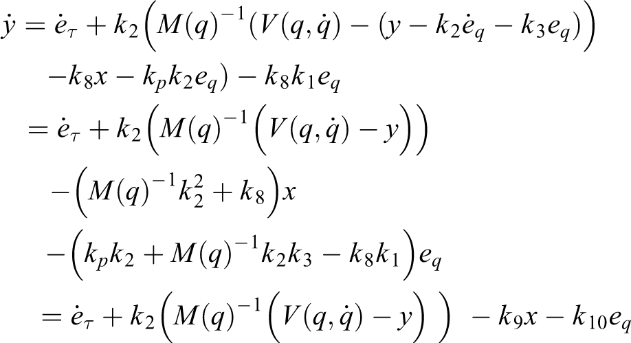
Let’s have the following constants with positive values as follows: $k_{1} = diag [k_{11}, \dots . k_{n 1}] > I_{5}, k_{2} = diag [k_{12}, \dots . k_{n 2}] > I_{5}, k_{3} = diag [k_{13}, \dots . k_{n 3}] > I_{5}, k_{3} > k_{2}$ , where I ₅ is 5 × 5 identity matrix. $k_{p} = diag [k_{1 p}, \dots . k_{n p}], k_{d} = diag [k_{1 d}, \dots . k_{n d}]$

$k_{5} = | k_{1} + k_{d} - M {(q)}^{- 1} k_{2} |$ , $k_{6} = | k_{p} - M {(q)}^{- 1} k_{3} |$ , $k_{7} = | k_{6} - k_{5} k_{1} |$ , $k_{8} = | k_{2} k_{d} - k_{3} |$ , $k_{9} = | M {(q)}^{- 1} k_{2} + k_{8} |$ , $k_{10} = | k_{p} k_{2} + M {(q)}^{- 1} k_{2} - k_{8} k_{1} |$ , where k ₅–k ₁₀ are 5 × 5 matrices.

In RAC-AFC controllers as shown in Figure 2, we have three loops of errors; first loop with K_p has an error equal to e_q . The errors in the second loop with K_d and third loop with AFC can be calculated as equations (21) and (22), respectively

x = {\dot{e}}_{q} + k_{1} e_{q}

y = e_{τ} + k_{2} {\dot{e}}_{q} + k_{3} e_{q}

The structure of KF-RAC-AFC feedback loops allows to eliminate robustly the effects of errors, in which the inner loops are compensating the errors very fast, with 10 times or higher than the outer loops.²⁹ Thus one can write

| e_{q} | ≫ | {\dot{e}}_{q} | ≫ | e_{τ} |

If we consider that k ₁, k ₂ and k ₃ are larger than identity matrix, and k ₃ is larger than k ₂ as mentioned previously, the plus/minus sign of e_q term will play the most significant role to determine the signs of x and y errors as in equations (21) and (22). As a result of that, the x and y errors will accordingly get the same sign either + or – along the controller operation time.

By deriving error x

\dot{x} = {\ddot{e}}_{q} + k_{1} {\dot{e}}_{q}

By substituting the value of ${\ddot{e}}_{q}$ from equation (19)

\dot{x} = M {(q)}^{- 1} (V (q, \dot{q}) - e_{τ}) - k_{d} {\dot{e}}_{q} - k_{p} e_{q} + k_{1} {\dot{e}}_{q}

By substituting the value of $e_{τ}$ from equation (22)

\dot{x} = M {(q)}^{- 1} (V (q, \dot{q}) - (y - k_{2} {\dot{e}}_{q} - k_{3} e_{q}) - k_{d} {\dot{e}}_{q} - k_{p} e_{q} + k_{1} {\dot{e}}_{q}

By collecting the identical parts

\begin{matrix} \dot{x} = M {(q)}^{- 1} (V (q, \dot{q}) - y) - (k_{1} + k_{d} - M {(q)}^{- 1} k_{2}) {\dot{e}}_{q} \\ - (k_{p} - M {(q)}^{- 1} k_{3}) e_{q} \end{matrix}

\dot{x} = M {(q)}^{- 1} (V (q, \dot{q}) - y) - k_{5} {\dot{e}}_{q} - k_{6} e_{q}

By substituting the value of ${\dot{e}}_{q}$ from equation (21)

\dot{x} = M {(q)}^{- 1} (V (q, \dot{q}) - y) - k_{5} (x - k_{1} e_{q}) - k_{6} e_{q}

\dot{x} = M {(q)}^{- 1} (V (q, \dot{q}) - y) - k_{5} x - (k_{6} - k_{5} k_{1}) e_{q}

\dot{x} = M {(q)}^{- 1} (V (q, \dot{q}) - y) - k_{5} x - k_{7} e_{q}

By deriving error y

\dot{y} = {\dot{e}}_{τ} + k_{2} {\ddot{e}}_{q} + k_{3} {\dot{e}}_{q}

By substituting the value of ${\ddot{e}}_{q}$ from equation (19)

\begin{matrix} \dot{y} = {\dot{e}}_{τ} + k_{2} (M {(q)}^{- 1} (V (q, \dot{q}) - e_{τ}) - k_{d} {\dot{e}}_{q} - k_{p} e_{q}) - k_{3} {\dot{e}}_{q} \\ = {\dot{e}}_{τ} + k_{2} (M {(q)}^{- 1} (V (q, \dot{q}) - e_{τ}) - k_{p} e_{q}) - (k_{2} k_{d} - k_{3}) {\dot{e}}_{q} \\ = {\dot{e}}_{τ} + k_{2} (M {(q)}^{- 1} (V (q, \dot{q}) - e_{τ}) - k_{p} e_{q}) - k_{8} {\dot{e}}_{q} \end{matrix}

By substituting the value of ${\dot{e}}_{q}$ from equation (21)

\dot{y} = {\dot{e}}_{τ} + k_{2} (M {(q)}^{- 1} (V (q, \dot{q}) - e_{τ}) - k_{p} e_{q}) - k_{8} (x - k_{1} e_{q})

By substituting the value of $e_{τ}$ from equation (22)

\begin{matrix} \dot{y} = {\dot{e}}_{τ} + k_{2} (M {(q)}^{- 1} (V (q, \dot{q}) - (y - k_{2} {\dot{e}}_{q} - k_{3} e_{q})) \\ - k_{8} x - k_{p} k_{2} e_{q}) - k_{8} k_{1} e_{q} \\ = {\dot{e}}_{τ} + k_{2} (M {(q)}^{- 1} (V (q, \dot{q}) - y)) \\ - (M {(q)}^{- 1} k_{2}^{2} + k_{8}) x \\ - (k_{p} k_{2} + M {(q)}^{- 1} k_{2} k_{3} - k_{8} k_{1}) e_{q} \\ = {\dot{e}}_{τ} + k_{2} (M {(q)}^{- 1} (V (q, \dot{q}) - y)) - k_{9} x - k_{10} e_{q} \end{matrix}

The quadratic Lyanupov function can be defined as follows

V = \frac{1}{2} e_{q}^{2} + \frac{1}{2} x^{2} + \frac{1}{2} y^{2} + x y

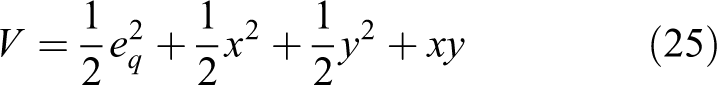
where x and y have the same +/− sign as have been explained previously. Equation (25) can be written in the matrix form as follows

V = \frac{1}{2} e_{q}^{T} e_{q} + \frac{1}{2} x^{T} x + \frac{1}{2} y^{T} y + x^{T} y

\dot{V} = e_{q} {\dot{e}}_{q} + x \dot{x} + y \dot{y} + \dot{x} y + x \dot{y}

Equation (26) can be written in the matrix form as follows

\begin{matrix} \dot{V} = e_{q}^{T} {\dot{e}}_{q} + x^{T} \dot{x} + y^{T} \dot{y} + y^{T} \dot{x} + x^{T} \dot{y} \\ = e_{q}^{T} (x - k_{1} e_{q}) + x^{T} (M {(q)}^{- 1} (V (q, \dot{q}) - y) - k_{5} x - k_{7} e_{q}) \\ + y^{T} ({\dot{e}}_{τ} + k_{2} (M {(q)}^{- 1} (V (q, \dot{q}) - y)) - k_{9} x - k_{10} e_{q}) \\ + y^{T} (M {(q)}^{- 1} (V (q, \dot{q}) - y) - k_{5} x - k_{7} e_{q}) \\ + x^{T} ({\dot{e}}_{τ} + k_{2} (M {(q)}^{- 1} (V (q, \dot{q}) - y)) - k_{9} x - k_{10} e_{q}) \\ = e_{q}^{T} x - e_{q}^{T} k_{1} e_{q} + x^{T} M {(q)}^{- 1} V (q, \dot{q}) - x^{T} M {(q)}^{- 1} y \\ - x^{T} k_{5} x - x^{T} k_{7} e_{q} + y^{T} {\dot{e}}_{τ} + y^{T} k_{2} M {(q)}^{- 1} V (q, \dot{q}) - y^{T} k_{2} M {(q)}^{- 1} y \\ - y^{T} k_{9} x - y^{T} k_{10} e_{q} + y^{T} M {(q)}^{- 1} V (q, \dot{q}) - y^{T} M {(q)}^{- 1} y - y^{T} k_{5} x - y^{T} k_{7} e_{q} \\ + x^{T} {\dot{e}}_{τ} + x^{T} k_{2} M {(q)}^{- 1} V (q, \dot{q}) - x^{T} k_{2} M {(q)}^{- 1} y - x^{T} k_{9} x - x^{T} k_{10} e_{q} \\ = - e_{q}^{T} k_{1} e_{q} - x^{T} (k_{5} + k_{9}) x - y^{T} M {(q)}^{- 1} (k_{2} + 1) \\ - x^{T} M {(q)}^{- 1} (k_{2} + 1) y - y^{T} (k_{9} + k_{5}) x + (e_{q}^{T} x + x^{T} M {(q)}^{- 1} V (q, \dot{q}) \\ - x^{T} k_{7} e_{q} + y^{T} \dot{e_{τ}} + y^{T} k_{2} M {(q)}^{- 1} V (q, \dot{q}) - y^{T} k_{10} e_{q} + y^{T} M {(q)}^{- 1} V (q, \dot{q}) \\ - y^{T} k_{7} e_{q} + x^{T} \dot{e_{τ}} + x^{T} k_{2} M {(q)}^{- 1} V (q, \dot{q}) - x^{T} k_{10} e_{q}) \end{matrix}

If ${\dot{e}}_{τ}$ is changing with a constant rate and fixed sampling time in the whole experiment, this will bound ${\dot{e}}_{τ}$ as follows

∥ {\dot{e}}_{τ} ∥ \leq δ

where δ is the first derivative of the torque error.

If M(q) or IN is bounded in a FL system as in equation (15), and ${\dot{φ}}^{2}$ in $V (q, \dot{q})$ is also changed with a constant rate $(\dot{φ} = constant)$ , this will cause the ratio $M {(q)}^{- 1} V (q, \dot{q})$ is also bounded too.

The derivation of Lyapunov function as in equation (26) can then be written as

\dot{V} = - α V + C

where α is the minimum factors of x, y and xy.

\begin{matrix} C = \underset{t \to \infty}{Sup} (e_{q}^{T} x + x^{T} M {(q)}^{- 1} V (q, \dot{q}) - x^{T} k_{7} e_{q} + y^{T} {\dot{e}}_{τ} \\ + y^{T} k_{2} M {(q)}^{- 1} V (q, \dot{q}) - y^{T} k_{10} e_{q} + y^{T} M {(q)}^{- 1} V (q, \dot{q}) \\ - y^{T} k_{7} e_{q} + x^{T} {\dot{e}}_{τ} + x^{T} k_{2} M {(q)}^{- 1} V (q, \dot{q}) - x^{T} k_{10} e_{q}) \end{matrix}

According to the above-mentioned Lemma, the closed-loop control system is guaranteed to reach the global uniform ultimate boundedness with exponential-convergence-rate of V specified by α.

Path control simulation

The simulation is accomplished considering a roundabout setting in MATLAB [R2016a] computing environment, where the robot is navigating autonomously from starting to goal positions. The RAC-AFC control scheme has been applied to enable the robot to track the planned path with small tracking errors.

Mobile robot path planning

With the novel path planning algorithm, the so-called laser simulator graph search approach,^28,30,31,32 the collision-free path is determined in a roundabout environment. The start and goal points of the path are pre-chosen by the user to drive the robot in a roundabout with 360° rotation while avoiding the obstacles as shown in Figure 4.

Figure 4.

Predefined path of mobile robot: (a) principle of laser simulator; (b) free-collision path with one obstacle.

Robot path control

The simulation for the predefined path as shown in Figure 4(b) was performed using MATLAB/Simulink according to the following conditions:

Integration algorithm: BogackiShanpine

Simulation type: Fixed step size

WMR parameters: r = 0.15 m, b = 0.75 m, d = 0.03 m, m = 31.0 kg, m _w = 0.5 kg, I = 15.625 kg m², I _w = 0.005 kg m²

Controller parameters: K _px = 2/s², K _py = 2/s², K _p = 2/s, K _dx = 1, K _dy = K _d = 1 (for the RACpart), K _t = [0.265 0.265]^T

N/A (obtained from datasheet for the DC motor)

Several disturbances with constant and harmonic torques were applied at both left and right wheels of the robot to test the performance of the control system. Three types of controllers were used in the simulation work, namely, the RAC-based kinematic controller, AFC-based dynamic controller and RAC-AFC controller, which were subsequently compared using a referenced trajectory.

Figure 5 shows the actual trajectory of all the controllers without disturbance during the robot tracking along the predefined path as depicted in Figure 4. RAC presents the reckoning errors that are incrementally increased during the tracking of the path with high tracking errors of about 30 mm and 35 mm in x and y axes, respectively. However, the differences between the referenced and actual paths generated by the AFC and RAC-AFC schemes are too small; the tracking errors were in the region of 10⁻² mm.

Figure 5.

Results of the RAC, AFC and RAC-AFC controllers without disturbance: (a) trajectory of mobile robot; (b) y track errors for all controllers; (c) y track errors for AFC and RAC-AFC; (d) x track errors for all controllers; (e) x track errors for AFC and RAC-AFC. RAC: resolved=acceleration control; AFC: active force control.

It was noticed that large initial errors (overshoots) occurred at the beginning of the simulation period for the AFC controller since there are as yet still no output signals received from the AFC controller loop at that point in time, whereas for the RAC and RAC-AFC schemes, there was no noticeable overshoots due to the positive effects of the kinematic control action at the beginning of the motion.

Figure 6 shows the actual trajectory of all the three controllers with the application of constant disturbance torques to both wheels, $τ_{d} = {[0.1 0.1]}^{T}$ Nm as the mobile robot navigates the predefined path.

Figure 6.

Results of the RAC, AFC and RAC-AFC controllers with disturbance, 0.1 Nm at both wheels: (a) trajectory of mobile robot; (b) x track errors; (c) y track errors. RAC: resolved-acceleration control; AFC: active force control.

For the second case of applying harmonic disturbance torques at both wheels with τ _d = [10000 sin(t) 10000 cos(t)]^T Nm, the RAC approach presents big deviation in the errors of about 50 mm and 60 mm in x and y directions, respectively, during tracking. Similar to the first case, the tracking errors for the AFC and RAC-AFC controllers remain very small, also in the region of 10⁻² mm for both x and y directions. Figure 7 shows the actual trajectory of the AFC and RAC-AFC controllers with harmonic disturbance applied to the robot moving in the same the predefined path as shown in Figure 4.

Figure 7.

Results of the AFC and RAC-AFC controllers with harmonic disturbance $τ_{d} = [\begin{array}{l} 10000 sin (t) \\ 10000 cos (t) \end{array}]$ Nm: (a) trajectory of mobile robot; (b) x track errors; (c) y track errors. RAC: resolved-acceleration control; AFC: active force control.

The third case considers only the AFC-based schemes.

The performance of such systems in terms of the tracking errors is quite obvious; the errors for the AFC controllers are in the region of 10⁻² mm in the x and y directions, more so for the RAC-AFC scheme that exhibits much smaller tracking errors (about 10⁻³ mm or less in both x and y directions).

Figure 8 shows a comparison between the actual trajectory of RAC-AFC controller and reference trajectory without and with harmonic disturbances, $τ_{d} = {[10, 000 cos (t) 10, 000 sin (t + \frac{π}{2})]}^{T} Nm$ applied to both wheels of the mobile robot. The tracking errors with/without disturbance are too small. The tracking errors in the x direction for RAC-AFC with/without disturbance are illustrated in Figure 8(a) are in the region of 10⁻⁴ mm with maximum errors of 2.5 × 10⁻⁴ mm and 0.5 × 10⁻⁴ mm with and without disturbances, respectively. In the y direction, the tracking errors have maximum value of about 5 × 10⁻⁴ mm and 4 × 10⁻⁴ mm with and without disturbances, respectively, as shown in Figure 8(b). It can be said that the RAC-AFC controller shows a higher degree of disturbance rejection among all controllers.

Figure 8.

Results produced by the RAC-AFC controller for both with and without disturbances: (a) x-tracking errors; (b) y-tracking errors. RAC: resolved-acceleration control; AFC: active force control.

Experimental path control

The mobile platform was set to move at a relatively low speed, typically in the range of 0.2–1.5 m/s. This range is in fact applicable to vehicles that are normally used for road service applications such as road painting, side road grass cutting and cleaning. A COM server communication was utilized to transmit and receive the data online through programming using Visual C-sharp [Visual C# 2010 Express] as client and MATLAB computing platform as the server.

The KF algorithm was computed in MATLAB via the same m-file script, where the signal and image processing sections were numerically processed. The Simulink program was then linked to the m file for calculating the AFC parameters. Figure 9 shows the link between MATLAB (as server) and C-sharp (as client) using the COM automation server with appropriate connections to the sensors and actuators.

Figure 9.

Software communication with sensors and actuators.

The path of the mobile robot is controlled using the RAC-AFC strategy as presented in the second section. Considering similar conditions with that of the path control simulation, two feedback loops were used in the control scheme, that is, the external and internal loops. The former is used for controlling the kinematic parameters by the RAC, while the latter for controlling the robot dynamics by the AFC controller. RAC controller is known as the outer loop of the RAC-AFC control system and in the AFC controller, the torque applied at the driving wheels was estimated in real time during movement. The encoders were used to numerically estimate the angular acceleration (via second derivative of the angular position) of the wheels. The signals were then multiplied with the estimated inertia matrix to calculate the required actuated torque, again through a signal processing task. This signal in turn is compared with the applied torque as expressed in equation (14). The torque of the selected DKM-DC motor used in this project has a linear relationship with the current and angular speed characteristic as shown in Figure 10. Note that the torque was calculated according to the angular speed characteristic. By getting the speed from encoders and taking into consideration the gear ratio, the equation that calculates the applied torque can be written as follows

τ = K_{n} μ n

where K _n is a torque constant, the value of which is obtained as 0.00108 Nm/r/min after unit conversion and derived from the datasheet of the selected motor (see Figure 10). µ = 1:30 is the gearbox ratio, again taken from the catalogue of the selected motor. n r/min is the speed of the wheel measured by the encoder which can be calculated as follows

n = \frac{P_{cur}^{​}}{T P_{rf}}

where P _cur is the number of pulses for the whole movement of robot from the start to current positions, P _rf is the number of pulses for one full rotation, T is the period (or sampling time) from the start to current positions. Thus, by getting the encoders measurements and then multiplied them with K _n and µ, the applied torque computed by the DC motors can be estimated and controlled. The acceleration can be calculated from the encoders’ measurements as second derivatives of the positions between two successive measurements as formulated in equation (30)

a = \frac{\partial_{2} (x_{2} - x_{1})}{\partial T^{2}}

Figure 10.

DKM motor (120 W) characteristic.

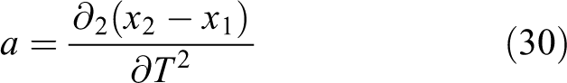
By estimating the inertia matrix using a suitable method, the controller can effectively compensate the disturbances. In this practical experimentation, FL method was also implemented. The disturbances in the AFC controller can be estimated using equation (14). The FL linguistic variables and membership functions, which were used to estimate the inertia matrix are shown in Tables 1 and 2 and Figure 11.

Table 1.

Fuzzy input variable, ϕ

Variable: ϕ (°)
Very low (VL)	−6.7 to −4.8
Low (L)	−4.8 to −3.3
Medium (M)	−3.3 to −1.9
High(H)	−1.9 to −0.45
Very high (VH)	−0.45 to 1

Table 2.

Fuzzy output variables, INL and INR.

Variables: INL and INR [kg m²]
Very small (VS)	0.27–0.30
Small (S)	0.30–0.33
Medium (M)	0.33–0.36
Large (L)	0.36–0.40
Very large (VH)	0.40–0.43

Figure 11.

FL rule interface and membership functions of the FL system with reference to the input and output: (a) input (ϕ); (b) output INR/INL. FL: fuzzy logic.

The input fuzzy set is:

ϕ = {Very Low, Low, Medium, High, Very High}

The output fuzzy sets are:

INR/INL = {Very Small, Small, Medium, Large, Very Large}

Propagation of kinematic uncertainty using KF

KF is a recursive data processing algorithm that can be used for stochastic estimation of the noisy sensor measurements. The linear and heading velocities of the WMR described by equations (5) and (7), respectively, are considered as the control input of the KF, that is, u = [V, $\dot{φ}$ ]^T.

In the process state, the state variable vector, q = [x, y, ϕ]^T is calculated by the average velocity as expressed in equation (31). The direct KF was implemented in which the measurement signals from the odometry device, camera and LRF were combined and transformed into a single measurement vector, Z _k as presented in equation (33), which is then fed into the KF algorithm. The linear discrete time of the state variable that describes the time update step for the KF can be written as follows

q_{k}^{-} = A q_{k - 1}^{​} + B u_{k} + B w

If the sampling period is small enough and both the linear and angular velocities are assumed to be constant throughout the duration, the position state variable of the non-holonomic WMR within its environments in the presence of the uncertainties in discrete time is

[\begin{array}{l} x_{k} \\ y_{k} \\ φ_{k} \end{array}] = [\begin{matrix} 1 & 0 & 0 \\ 0 & 1 & 0 \\ 0 & 0 & 1 \end{matrix}] [\begin{array}{l} x_{k - 1} \\ y_{k - 1} \\ φ_{k - 1} \end{array}] + \nabla T [\begin{matrix} cos(φ) & - dsin(φ) \\ sin(φ) & dcos(φ) \\ 0 & 1 \end{matrix}] [\begin{array}{l} V + w_{v} \\ \dot{\dot{φ} + w_{φ}} \end{array}]

The KF measurement equation with noise is

Z_{k} = C q_{k}^{​} + v_{k}

The equation that describes the sensor model in WMR is thus

[\begin{array}{l} x_{k}^{​} \\ y_{k} \\ φ_{k} \end{array}] = [\begin{array}{l} 1 0  0 \\ 0  1  0 \\ 0 0  1 \end{array}] [\begin{array}{l} x_{k} from LRF \\ y_{k} from odometry \\ φ_{k} from mixed LRF, Odometry and LS \end{array}] + [\begin{array}{l} v_{1} \\ v_{2} \\ v_{3} \end{array}]

In the real-world application, the values of Q _k and R _k are not constant and always changing with each time step.

Thus, the actual process and measurement noises are not a zero-mean white noise which in turn renders the residual in KF a non-white noise. For this reason, the KF would diverge or tend to produce a large bound. To avoid this condition, the exponentially weighted moving averages were used to estimate the discrete time-varying system covariance from the noisy measurements in KF³³ as follows

R_{k} = R ξ^{- k - 1} and Q_{k} = Q ξ^{- k - 1} where ξ > 1

Note that Q and R are constant values. In this study, we assume Q = [0.001 0.001 0.001]^T and R = [1 1]^T after a number of trial runs. For different values of ξ (from 1 to 5), the mean trajectory errors after applying KF are computed as shown in Table 3.

Table 3.

Empirical calculation of ξ.

ξ	Mean difference between the trajectory before and after using KF (mm)
1	31.3
2	28.8
3	26.7
4	29.6
5	30.5

KF: Kalman Filter.

From the table, ξ is chosen as 3 since KF produces the smallest divergence.

The KF gain that shows how much the estimation must be corrected can be computed from the measurement using

K_{k} = P_{k}^{-} C^{T} {(C P_{k}^{-} C^{T} + R_{k})}^{- 1}

A posteriori state is generated by incorporating the measurement with the priori values of the state variable as

q_{k} = q_{k}^{-} + K_{k} (Z - C q_{k} ​^{-})

The priori and posteriori error covariance estimations can be calculated from equations (38) and (39), respectively, as follows

P_{k}^{-} = A P_{k - 1} A^{T} + Q_{k}

P_{k} = (I - K_{k} C) P_{k}^{-}

Experimental results and discussion

The laser range finder, encoders and cameras data as in previous studies^24
–26 were used to localize, determine the path and control the robot in a road roundabout environment as shown in Figure 12.

Figure 12.

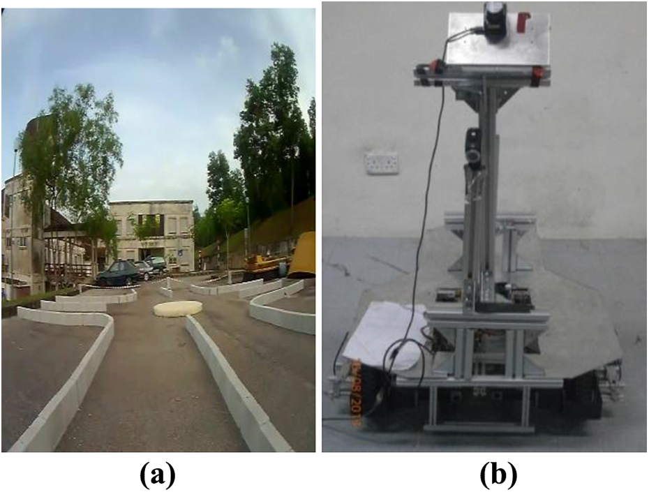
Outdoor roundabout environment: (a) Road roundabout and (b) mobile robot platform used in the experiments.

The image processing algorithm consists of two main parts; that is, preprocessing of the image and processing of the image and local map building. The image processing algorithm is listed here and more details can be found in previous studies,^28,34

(i) Preprocessing of the image

The main operations that were used in this phase are listed as follows:

– Constructing the video input object

– Preview of the Wi-Fi video

– Setting the brightness of live video

– Start acquiring frames

– Acquiring the image frames to MATLAB workspace

– Crop image

– Convert from RGB to grayscale

– Remove image acquisition object from memory

(ii) Processing of the image and development of the environments local map

It includes some operations that allow the extraction of the road edges and roundabout from the images with capability to remove the noises and perform filtration. The following operations were applied for edge detection and noise filtering:

– 2-D Gaussian filters

– Multidimensional images (imfilter)

– Prewitt filter for edge detection

– Morphological operations:

Morphological structuring element: It is used to define the areas that will be applied using morphological operations. Straight lines with 0° and 90° are the shapes used for the images which actually represent the road curbs.

Dilation of image: In the dilation process, a number of pixels are added to the boundaries of the objects in the image, which depends on the size and shape of the structuring element that is used to process the image.

BWC is the binary image coming from the edge filters.

– 2-D order-statistic filtering

– Removing of small objects from binary image

– Filling of the image regions and holes

The results of the preimage and image processing are illustrated in Figures 13 and 14.

Figure 13.

Navigating on the road following section in indoor environment using camera image sequences: (a) original image in the first iteration, (b) image after preprocessing and processing at the start position, (c) image after preprocessing and processing at the goal position path.

Figure 14.

Camera sequence images when navigating in outdoor environment with 360° rotation (a) image when start moving, (b) camera’s local map when robot starts to move, (c) camera’s local map when robot detects the roundabout.

The signal measurements of the odometry and LRF were used to estimate the position and orientation of the robot in road following and roundabout environments with 360° rotation as shown in Figure 15. These measurements include some unexpected noises and errors that can be effectively avoided after using KF and RAC-AFC controller. Figures 15(b) to (d) show the effect of applying KF with AFC controller to enhance the robot path in comparison with the path planning from signal measurement. Figure 16 shows the track errors of RAC-AFC controller in which for the x direction, a maximum error of about 7 × 10⁻⁵ mm is attained as shown in Figure 16(a).

Figure 15.

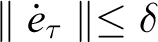
Path of mobile robot during navigation through the roundabout environment: (a) comparison between the path acquired from sensors signals before and after using KF and RAC-AFC controller, (b) comparison between the KF path and RAC-AFC controller, (c) KF path, (d) AFC controller path. RAC: resolved-acceleration control; AFC: active force control; KF: Kalman Filter.

Figure 16.

Track errors of the RAC-AFC controller: (a) x-track errors (b) y-track errors. RAC: resolved-acceleration control; AFC: active force control.

However, in y direction, the maximum track error is around 6 × 10⁻⁴ mm (Figure 16(b)). Although the experiments show that the complete navigation method enables the robot to move smoothly in the road environments in comparison to the direct path execution, the resulted path is not smooth and contains many ripples that may be due to the time needed to perform the path planning, localization and control calculations

The parameters used in the calculation are as follows:

WMR parameters: r = 105.4 mm, b = 500 mm, d = 16.5 mm, m = 36 kg, m _w= 1.5 kg, I =10.0567 kg m², I _w = 0.0083 kgm2, V = 0.15 m/s;

Controller parameters: K _px = 2/s², K_py = 2/s², K _p = 2/s, K _dx = K _dy = K _d = 1, K _n = 0.00108 Nm/r/min.

Conclusion

The RAC, AFC, RAC-AFC and RAC-AFC-KF controllers were used to navigate the robot and track the predefined roundabout trajectory both in simulation and in experimental studies. The parameters of the controllers were derived from the kinematic and dynamic models that fully describe the mobile robot motion with non-holonomic constraints. The FL reasoning was implemented to estimate the inertia matrix leading to the computation of the applied torque to drive the WMR wheels. From the results of simulation, it looks as if there are no noticeable errors for without disturbance condition. However, a small deviation (error) was observed with the application of constant or harmonic disturbances. In the experimental works, a drift between the actual and reference paths occurred due to the delay in processing the data from the sensors and noises, the latter of which were eliminated using KF. In conclusion, it is shown that the RAC-AFC-KF controller has demonstrated its capability to eliminate the disturbances and noises from the system both in simulation and experimental works.

Footnotes

Declaration of conflicting interests

The author(s) declared no potential conflicts of interest with respect to the research, authorship, and/or publication of this article.

Funding

The author(s) received no financial support for the research, authorship, and/or publication of this article.

ORCID iD

Mohammed AH Ali

References

Asif

Khan

Safwan

. Feedforward and feedback kinematics controller for wheeled mobile robot trajectory tracking. J Autom Control Eng 2015; 3(3): 178–182.

Gunes

Baba

. Speed and position control of autonomous mobile robot on variable trajectory depending on its curvature. J Sci Ind Res 2009; 68: 513–521.

Lee

Hung

FHF

Tam

PKS

. Position control for wheeled mobile robots using a fuzzy logic controller. Hong Kong: The Hong Kong Polytechnic, University, Hung Hom, Kowloon, 2002.

Astudillo

Castillo

Melin

. Intelligent control of an autonomous mobile robot using type-2 fuzzy logic. Mexico: Division of Graduate Studies and Research in Tijuana Institute of Technology, 2006.

Velagic

Osmic

Lacevic

. Neural network controller for mobile robot motion control. World Acad Sci Eng Technol 2008; 2(11): 47.

Borensteinand

Koren

. Motion control analysis of a mobile robot. J Dyn Sys Meas Control 1987; 109(2): 73–79.

Mester

. Intelligent mobile robot motion control in unstructured environments. Acta Polytechnica Hungarica 2010; 7(4): 153–165.

Kanayama

Kimura

Miyazaki

. A stable tracking control method for a non-holonomic mobile robot. In: Proceeding IEEE/RSJ international workshop on intelligent robots and systems, Osaka, Japan, 3–5 November 1991, pp 1236–1241. IEEE.

Blochs

Drakunov stabilization of a non-holonomic system via sliding modes. In: Proceedings of the 33rd Conference on Decision and Control, Lake Buena Vista, FL, 14–16 December 1994. IEEE.

10.

Chwa

. Sliding-mode tracking control of non-holonomic wheeled mobile robots in polar coordinates. IEEE Trans Contr Syst Trans 2004; 12(4): 637–644.

11.

Fierro

Lewis

. Control of a non-holonomic mobile robot: back stepping kinematics into dynamics. J Robot Syst 1997; 14(3): 149163.

12.

Fukao

Nakagawa

Adachi

. Adaptive tracking control of a non-holonomic mobile robot. IEEE Trans Robot Autom 2000; 16(5): 609–615.

13.

Jiangt

henk

. Tracking control of mobile robots: a case study in back stepping. Automatica 1997; 33(7): 1393–1399.

14.

Hendzel

. An adaptive critic neural network for motion control of a wheeled mobile robot. Nonlinear Dyn 2007; 50: 849.

15.

Fateh

Arab

. Robust control of a wheeled mobile robot by voltage control strategy. Nonlinear Dyn 2015; 79: 335.

16.

Hewit

Burdess

. Fast dynamic decoupled control for robotics using active force control. Trans Mech Mach Theory 1981; 16(5): 535–542.

17.

Hewit

Marouf

. Practical control enhancement via mechatronics design. IEEE Trans Ind Electron 1996; 43(1): 16–22.

18.

Mailah

Intelligent active force control of a rigid robot arm using neural network and iterative learning algorithms. PhD Thesis, University of Dundee, UK, 1998.

19.

Kwek

Wong

Loo

. Application of active force control and iterative learning in a 5-link biped robot. J Intell Robot Syst 2003; 37: 143–162.

20.

Luh

JYS

Walker

Paul

RPC

. Resolved acceleration control of mechanical manipulator. IEEE Trans Automat Contr 1980; 25: 486–474.

21.

Pitowarno

Mailah

Jamaluddin

. Knowledge-based trajectory error pattern method applied to an active force control scheme. IIUM Engineering Journal 2002; 3(1): 1–15.

22.

Tang

Mailah

Jalil

MKA

, Robust intelligent active force control of non-holonomic wheeled mobile robot. J Teknologi 2006; 44(D): 4964.

23.

Luy

. Omnidirectional vision-based distributed optimal tracking control for mobile multi-robot systems with kinematic and dynamic disturbance rejection. IEEE Trans Ind Electron 2018; 65(7): 5693–5703.

24.

Luy

. Robust adaptive dynamic programming based online tracking control algorithm for real wheeled mobile robot with omni-directional vision system. Trans Ins Meas Control 2017; 39(6): 832–847.

25.

Luy

. Reinforcement learning-based intelligent tracking control for wheeled mobile robot. Trans Ins Meas Control 2014; 36(7): 868–877.

26.

Chao

Chengrui

Tianliang

. Model-assisted extended state observer-based computed torque control for trajectory tracking of uncertain robotic manipulator systems. Int J Adv Robot Syst 2018; 15(5): 1–12.

27.

Boukattaya

Mezghani

Damak

. Computed-torque control of a wheeled mobile manipulator. Int J Robot Eng 2018; 3(5): 1–6.

28.

Mohammed

AHA

. Autonomous mobile robot navigation and control in the road following and roundabout environments incorporating laser range finder and vision system. PhD Thesis, Universiti Teknologi Malaysia, Malaysia, 2014.

29.

William

. Control system applications. Boca Raton: CRC Press, Technology & Engineering, 2018.

30.

Mohammed

AHA

Mailah

Hing

. Path navigation of mobile robot in a road roundabout setting. In: 1st International Conference on Systems, Control, Power, Robotics (SCOPORO’12) WSEAS, Singapore City, Singapore, 11–13 May 2012, pp. 198–203.

31.

Mohammed

AHA

Mailah

Hing

. Path planning of mobile robot for autonomous navigation of road roundabout intersection. Int J Mech 2012; 6(4): 203–211.

32.

Ali

MAH

Mailah

. Laser simulator: a novel search graph-based Path planning. Int J Adv Robot Syst 2018; 15(5): 1–16.

33.

Lewis

. Optimal Estimation with an introduction to stochastic control theory. New York: John-Wiley and Sons, 1986.

34.

Ali

MAH

Mailah

Yussof

WAB

. Sensors fusion based online mapping and features extraction of mobile robot in the road following and roundabout. IOP Conf Ser Mater Sci Eng 2016; 114(1): 012135.

A simulation and experimental study on wheeled mobile robot path control in road roundabout environment

Abstract

Keywords

Introduction

Modelling the non-holonomic WMR

Mobile robot kinematics

Mobile robot dynamics

Controller design

RAC control strategy

AFC control strategy

Estimation of inertial matrix

Stability analysis of RAC-AFC

Lemma

Theorem

Proof

Path control simulation

Mobile robot path planning

Robot path control

Experimental path control

Propagation of kinematic uncertainty using KF

Experimental results and discussion

Conclusion

Footnotes

Declaration of conflicting interests

Funding

ORCID iD

References