Sage Journals: Discover world-class research

Abstract

Balancing control of a rotary double inverted pendulum system is a challenging research topic for researchers in dynamics control field because of its nonlinear, high degree-of-freedom, under actuated and unstable characteristics. The system always works under uncertainties and disturbances. Many control algorithms fail or ineffectively control the rotary double inverted pendulum system. In this article, mixed sensitivity H∞ control is proposed to balance the rotary double inverted pendulum system. The controller is proposed to ensure the robust stability and enhance the time domain performance of the system under uncertainties and disturbances. Structure of the system, dynamics model and controller synthesis are presented. For performance evaluation, the proposed mixed sensitivity H∞ controller is compared with linear quadratic regulator from both simulation and experiment on the rotary double inverted pendulum system. The results show high performance of the proposed controller on the rotary double inverted pendulum system with model uncertainties and external disturbances.

Keywords

H∞ controller model uncertainties mixed sensitivity rotary double inverted pendulum weighting functions selection

Introduction

Inverted pendulum system is a nonlinear, under actuated and unstable system. It has been used in control field to evaluate control performance and efficiency of several controllers. The inverted pendulum system can be classified into two groups, that is, moving cart type and rotary type. Researches of the moving cart type are reviewed as follows. Andreas Siuka and Markus Schöberl,¹ Linden and Lambrechts,² and Cheang and Chen³ demonstrated how to control the single inverted pendulum on moving cart systems. The single inverted pendulum on moving cart system consists of only a pendulum and a moving cart in the system, which is the simplest inverted pendulum system. The system becomes more complicated with more pendulums in the system. Double inverted pendulum system may have serially connected two pendulums on a moving cart. Gretchen et al.⁴ and Liu and Zhou⁵ implemented and controlled this type of system. The other type of the double inverted pendulum system has two parallel pendulums on a moving cart. Nan Lu⁶ developed and controlled this type of system. The control concept of inverted pendulum was applied to design a controller to balance rockets during a vertical take-off by Kurode et al.⁷

Research works of the rotary type inverted pendulum systems are reviewed as follows. In Sukontanakarn and Parnichkun,⁸ a rotary single inverted pendulum system was successfully controlled using optimal control. Rotary dual inverted pendulum system with two parallel pendulums attached to a rotary arm was designed and controlled by Pakdeepattarakorn et al.⁹ In this article, a rotary double inverted pendulum (RDIP) system is developed and controlled. The system consists of serially connected two pendulums and a rotating arm driven by a motor. Balancing control of RDIP system is a challenging research topic for researchers in dynamics control field because of its nonlinear, high degree-of-freedom, under actuated and unstable characteristics. The system always works under uncertainties and disturbances.

Research works of RDIP system are reviewed as follows. The pole assignment method was proposed for periodic rotation of the outer pendulum while stabilizing the inner pendulum by Komine et al.¹⁰ An RDIP developed by Pan et al.¹¹ was controlled by using the conventional linear quadratic regulator (LQR). Casanova et al.¹² used an RDIP system to evaluate a multi-loop control structure for a multivariable plant with different delays in the signals between controller and plant.

H∞ control is a robust control approach. It is suitable when the system is subjected to influences of external disturbances as shown by Jiang et al.¹³ It has an ability to work in an inaccurate modeling and identification error system as shown in a pneumatic surgical robot system developed by Tuvayanond and Parnichkun.¹⁴ Various types of H∞ controllers have been designed. Some of them have been tested on inverted pendulum systems. After the introduction of H∞ norm by Zames,¹⁵ H∞ controller was developed by Doyle et al.¹⁶ It was applied to control a single inverted pendulum (SIP) on moving cart by Linden and Lambrechts.² They studied an influence of dry friction on the inverted pendulum system and achieved good performance using H∞ controller.

In addition to the original H∞ controller, some improvements and modifications of H∞ controller were introduced. H∞ loop shaping developed by McFarlane and Glover ¹⁷ was implemented by combining the conventional loop shaping method with H∞ controller. Cheang and Chen³ successfully controlled a single inverted pendulum on moving cart system by using the H∞ loop shaping. They proved that dynamic system under uncertainty was effectively controlled by loop shaping controller. Static H∞ loop shaping controller was applied to a double inverted pendulum on moving cart system by Liu and Zhou.⁵ Their loop shaping weighting functions were optimized by genetic algorithm. The other approach of designing H∞ controller is mixed sensitivity approach. To achieve good closed loop performances, such as disturbance rejection, noise attenuation, and control input bandwidth, the mixed sensitivity approach relies on optimization that involves two or more sensitivity functions, the sensitivity function (S), the input sensitivity function (KS), and the complementary sensitivity function (T) as reviewed by Kwakernaak.¹⁸ Thus mixed sensitivity approach can be differed mixed sensitivities, such as S/T in Peng et al.¹⁹ and M. Rachedi et al.,²⁰ S/KS in Wei-qian et al.,²¹ Ozana et al.,²² and Xinping Bao,²³ or S/KS/T in Alfaya et al.,²⁴ Bejarano et al.,²⁵ Delettre et al.,²⁶ Iannino et al.,²⁷ and Fragoso et al.²⁸ Peng et al.¹⁹ proposed H∞ controller to solve the S/T problem for the pneumatic manipulator with parameter variation, and low or high frequency disturbances acting on the pneumatic manipulator as uncertainties. Rachedi et al.²⁰ used mixed sensitivity controller for position control of a “Delta” parallel robot. The controller showed better performance against disturbance forces applied on the traveling plate compared to Proportional Integral Derivative (PID) controller. S/KS mixed sensitivity approach was applied for vibration control of high-order flexible structures by Wei-qian et al.²¹ The controller could satisfy tracking performance specification and internal stability. The same controller was also applied for elevation control of a helicopter by Ozana et al.²² Xinping Bao²³ developed a rudder-based roll control system for the robotic boat. They designed a mixed sensitivity H∞ controller to control yaw and roll attitude. Alfaya et al.²⁴ and Bejarano et al.²⁵ applied S/KS/T-based multivariable H∞ controller for one-stage refrigeration cycle. Their results showed better tracking performance and robustness against disturbance over PID and model predictive controller. The same controller was applied for a planar manipulator of flexible and contactless handling, steam turbine power generation applications, and a lab-scale wind turbine by Delettre et al.,²⁶ Iannino et al.,²⁷ and Fragoso et al.,²⁸ respectively. Their experiments showed better robust performance over the conventional controllers.

In this article, mixed sensitivity of S/KS/T H∞ is proposed to control a RDIP system. Control performance of the controller will be evaluated by both simulation and experiment on the nominal condition and the condition with external disturbances and parameter variation. In addition to robust stability, the other important control performance indices, including rise time, settling time, peak time, and peak value are also considered.

This article is organized as follows: in the second section, system architecture of the RDIP system is described. Mathematical model of the system is derived in the third section. A controller for the RDIP system is proposed and explained in the fourth section. Finally, the fifth section presents simulation and experimental results.

System architecture

Three-dimensional (3-D) model of the developed RDIP system is shown in Figure 1. The system consists of serially connected two pendulums mounted on an arm. Both pendulums can freely rotate about their pivot axes.

Figure 1.

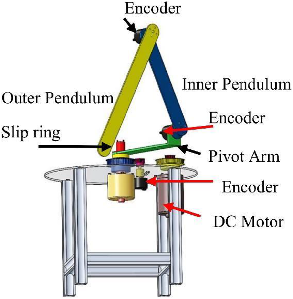
3-D model of the developed RDIP system. 3-D: three-dimensional; RDIP: rotary double inverted pendulum.

This under-actuated RDIP system has only one motor attached to the arm. The arm rotates on horizontal plane to balance both pendulums to the upright position on vertical axes. Photos of the developed RDIP system are shown in Figure 2.

Figure 2.

Photos of the developed RDIP system. RDIP: rotary double inverted pendulum.

The components of the RDIP system shown in Figure 2 are listed in Table 1. In real implementation, the arm and both pendulums are made from aluminum. Three optical encoders with resolution of 1024 pulses per revolution are utilized to measure the angular positions of the arm and both pendulums. The angular velocities of the arm and both pendulums are calculated by using data from the three encoders.

Table 1.

Components of RDIP system.

No.	Description	No.	Description
1	DC servomotor	6	Power supply
2	Encoders	7	Electrical design
3	Arm	8	Slip ring
4	Inner pendulum	9	Pulley and belt system
5	Outer pendulum	10	Mounting hub

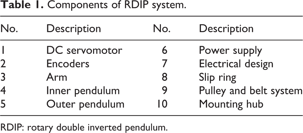
RDIP: rotary double inverted pendulum.

Two encoders are used to measure the angular positions of the pendulums and directly connected with the pendulums joints by using mounting hubs. The third encoder used to measure the angular position of the arm is connected with the motor by using pulley and belt as shown in Figure 3. Photos of some parts of the RDIP system are shown in Figure 4.

Figure 3.

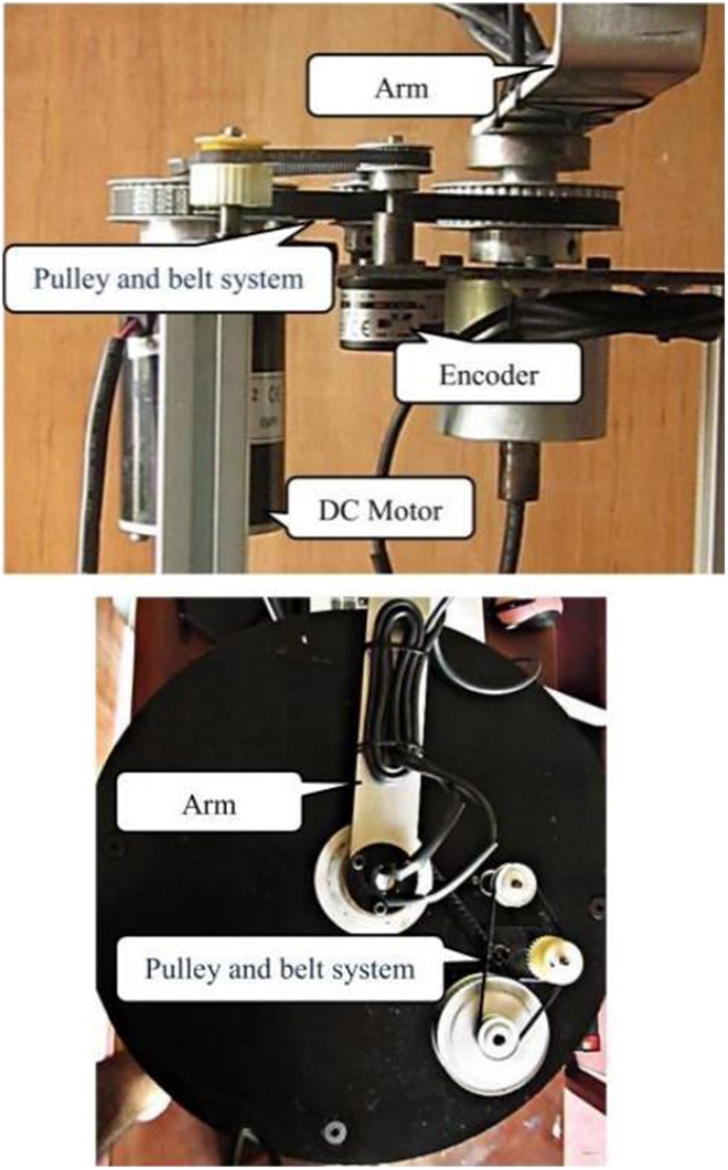
Belt and pulley transmission system.

Figure 4.

Parts of RDIP system. RDIP: rotary double inverted pendulum.

The arm of the RDIP system is driven by 150 W DC motor using belt and pulley transmission. In addition, since the system requires signals from the rotating arm, a slip ring is installed at the arm rotating axis. With this slip ring, the arm can be rotated freely without any constraints from the encoder wires. Parameters of the RDIP system are then identified. Some parameters are obtained from SOLIDWORKS program. Some parameters are obtained from direct measurement.

STM32F407 microcontroller with 32-bit ARM Cortex M4 core architecture is utilized to control the RDIP system. H-bridge DC motor driver with continuous current up to 80 A at 24 V capacity is applied to drive the DC motor.

Electrical circuit of the system is shown in Figure 5. Components of the electrical circuit are listed in Table 2.

Figure 5.

Electrical circuit board of RDIP system. RDIP: rotary double inverted pendulum.

Table 2.

Components of electrical circuit.

No.	Description	No.	Description
1	Motor driver board	4	DS26C32 IC
2	Encoder input connecters	5	Motor control signal connector
3	LM317 linear voltage regulator	6	Microcontroller

Dynamic model

Schematic diagram of the RDIP system is shown in Figure 6. Dynamics model of the system is derived using Euler–Lagrange equation of motion which is expressed as equation (1)

\frac{d}{d t} (\frac{\partial L}{\partial {\dot{q}}_{i}}) - \frac{\partial L}{\partial q_{i}} + \frac{\partial W}{\partial {\dot{q}}_{i}} = F_{i} i = 1, 2, \dots, m

where $q_{i} = [\begin{matrix} \emptyset_{A} \\ \emptyset_{I} \\ \emptyset_{O} \end{matrix}]$ , ${\dot{q}}_{i} = [\begin{matrix} {\dot{\emptyset}}_{A} \\ {\dot{\emptyset}}_{I} \\ {\dot{\emptyset}}_{O} \end{matrix}]$ , and $F_{i} = [\begin{matrix} τ \\ 0 \\ 0 \end{matrix}]$ .

Figure 6.

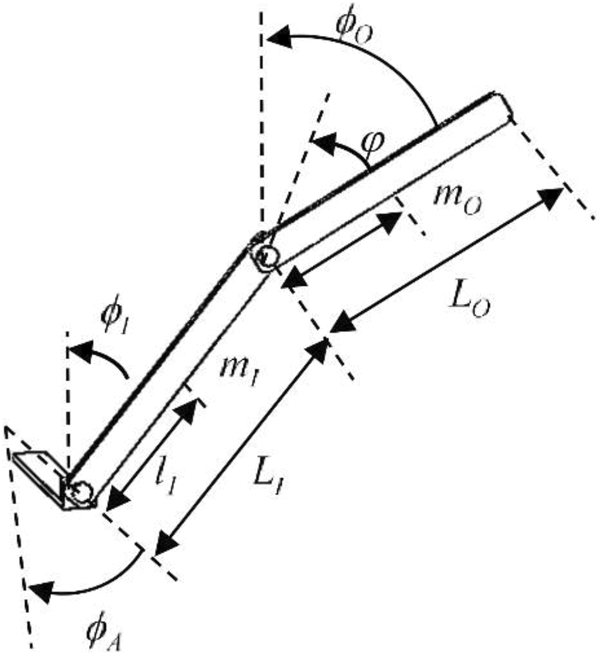
Schematic diagram of the system.

There are three equations are obtained from equation (1)

{\begin{matrix} \frac{d}{d t} (\frac{\partial L}{\partial {\dot{\emptyset}}_{A}}) - \frac{\partial L}{\partial \emptyset_{A}} + \frac{\partial W}{\partial {\dot{\emptyset}}_{A}} = τ \\ \frac{d}{d t} (\frac{\partial L}{\partial {\dot{\emptyset}}_{I}}) - \frac{\partial L}{\partial \emptyset_{I}} + \frac{\partial W}{\partial {\dot{\emptyset}}_{I}} = 0 \\ \frac{d}{d t} (\frac{\partial L}{\partial {\dot{\emptyset}}_{O}}) - \frac{\partial L}{\partial \emptyset_{O}} + \frac{\partial W}{\partial {\dot{\emptyset}}_{O}} = 0 \end{matrix}

In equations (1) and (2), Lagrangian (L), can be written as

L = \sum_{i = 1}^{3} T_{i} - \sum_{I = 1}^{3} V_{i}

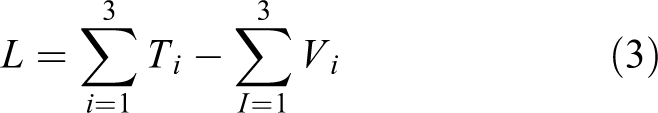
where $\sum_{i = 1}^{3} T_{i}$ is the total kinetic energy and $\sum_{i = 1}^{3} V_{i}$ is the total potential energy.

Notation: For clarity, the following notations are used throughout the article. (*)_A, (*)_I, and (*)_O represent parameters related to the arm, the inner pendulum, and the outer pendulum.

Total kinetic energy is the summation of the following kinetic energies.

Kinetic energy of the arm

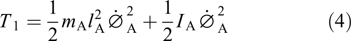
T_{1} = \frac{1}{2} m_{A} l_{A}^{2} {\dot{\emptyset}}_{A}^{2} + \frac{1}{2} I_{A} {\dot{\emptyset}}_{A}^{2}

When the distance between center of the mass and rotation axis of the rotating arm equals zero, kinetic energy becomes

T_{1} = \frac{1}{2} I_{A} {\dot{\emptyset}}_{A}^{2}

Kinetic energy of the inner pendulum

T_{2} = \frac{1}{2} m_{I} L_{A}^{2} {\dot{\emptyset}}_{A}^{2} + \frac{1}{2} (m_{I} l_{I}^{2} + I_{I}) {\dot{\emptyset}}_{I}^{2} + m_{I} L_{A} {\dot{\emptyset}}_{A} l_{I} {\dot{\emptyset}}_{I} cos \emptyset_{I}

Kinetic energy of the outer pendulum

T_{3} = \frac{1}{2} m_{O} L_{A}^{2} {\dot{\emptyset}}_{A}^{2} + \frac{1}{2} m_{O} L_{I}^{2} {\dot{\emptyset}}_{I}^{2} + \frac{1}{2} (m_{O} l_{O}^{2} + I_{O}) {\dot{\emptyset}}_{O}^{2} + m_{O} L_{A} L_{I} {\dot{\emptyset}}_{A} {\dot{\emptyset}}_{I} cos \emptyset_{I} + m_{O} L_{A} l_{O} {\dot{\emptyset}}_{A} {\dot{\emptyset}}_{O} cos \emptyset_{O} + m_{O} L_{A} l_{O} {\dot{\emptyset}}_{I} {\dot{\emptyset}}_{O} cos (\emptyset_{I} - \emptyset_{O})

From equations (5) to (7), total kinetic energy

\begin{matrix} \sum_{i = 1}^{3} T_{i} = \frac{1}{2} I_{A} {\dot{\emptyset}}_{A}^{2} + \frac{1}{2} m_{I} L_{A}^{2} {\dot{\emptyset}}_{A}^{2} + \frac{1}{2} (m_{I} l_{I}^{2} + I_{I}) {\dot{\emptyset}}_{I}^{2} + m_{I} L_{A} {\dot{\emptyset}}_{A} l_{I} {\dot{\emptyset}}_{I} cos \emptyset_{I} + \frac{1}{2} m_{O} L_{A}^{2} {\dot{\emptyset}}_{A}^{2} + \frac{1}{2} m_{O} L_{I}^{2} {\dot{\emptyset}}_{I}^{2} + \frac{1}{2} (m_{O} l_{O}^{2} + I_{O}) {\dot{\emptyset}}_{O}^{2} \\ + m_{O} L_{A} L_{I} {\dot{\emptyset}}_{A} {\dot{\emptyset}}_{I} cos \emptyset_{I} + m_{O} L_{A} l_{O} {\dot{\emptyset}}_{A} {\dot{\emptyset}}_{O} cos \emptyset_{O} + m_{O} L_{A} l_{O} {\dot{\emptyset}}_{I} {\dot{\emptyset}}_{O} cos (\emptyset_{I} - \emptyset_{O}) \end{matrix}

Total potential energy is the summation of the following potential energies.

Potential energy of the arm

V_{I} = 0

Potential energy of the inner pendulum

V_{2} = m_{I} g l_{I} cos \emptyset_{I}

Potential energy of the outer pendulum

V_{3} = m_{O} g (L_{I} cos \emptyset_{I} + l_{O} cos \emptyset_{O})

From equations (9) to (11), total potential energy

\sum_{I = 1}^{3} V_{i} = m_{I} g l_{I} cos \emptyset_{I} + m_{O} g (L_{I} cos \emptyset_{I} + l_{O} cos \emptyset_{O})

W is the energy lost in the system from viscosity friction. Total loss energy of the system can be expressed by using loss energy of the arm, inner pendulum, and outer pendulum

W = \frac{1}{2} C_{A} {\dot{\emptyset}}_{A}^{2} + \frac{1}{2} C_{I} {\dot{\emptyset}}_{I}^{2} + \frac{1}{2} C_{O} {\dot{\emptyset}}_{O}^{2}

Notation: First derivation and second derivation of the (*) are defined as $(\dot{*})$ and $(\ddot{*})$ , respectively. ${(\dot{*})}_{A}, {(\dot{*})}_{I}$ , and ${(\dot{*})}_{O}$ represent first derivation parameters related to the arm, the inner pendulum, and the outer pendulum.

In order to obtain dynamic model of the system, the Lagrangian of the RDIP system is derived by equation (3) and obtained as expressed in equation (14)

\begin{matrix} L = \frac{1}{2} I_{A} {\dot{\emptyset}}_{A}^{2} + \frac{1}{2} m_{I} L_{A}^{2} {\dot{\emptyset}}_{A}^{2} + \frac{1}{2} (m_{I} l_{I}^{2} + I_{I}) {\dot{\emptyset}}_{I}^{2} + m_{I} L_{A} {\dot{\emptyset}}_{A} l_{I} {\dot{\emptyset}}_{I} cos \emptyset_{I} + \frac{1}{2} m_{O} L_{A}^{2} {\dot{\emptyset}}_{A}^{2} + \frac{1}{2} m_{O} L_{I}^{2} {\dot{\emptyset}}_{I}^{2} + \frac{1}{2} (m_{O} l_{O}^{2} + I_{O}) {\dot{\emptyset}}_{O}^{2} \\ + m_{O} L_{A} L_{I} {\dot{\emptyset}}_{A} {\dot{\emptyset}}_{I} cos \emptyset_{I} + m_{O} L_{A} l_{O} {\dot{\emptyset}}_{A} {\dot{\emptyset}}_{O} cos \emptyset_{O} + m_{O} L_{A} l_{O} {\dot{\emptyset}}_{I} {\dot{\emptyset}}_{O} cos (\emptyset_{I} - \emptyset_{O}) - m_{I} g l_{I} cos \emptyset_{I} \\ - m_{O} g (L_{I} cos \emptyset_{I} + l_{O} cos \emptyset_{O}) \end{matrix}

Definitions of the parameters in equation (14) and their values are listed in Table 3.

Table 3.

System parameters and values.

	Values
Parameters/units	arm	Inner pend	Outer pend
m, mass (kg)	0.246	0.236	0.136
C, viscous coefficient (N·ms)	0.05035	0.24915	0.24490
L, length (m)	0.229	0.310	0.410
l, Distance to the center of mass (m)	0.1579	0.14504	0.16539
I, inertia (kg m²)	0.02358	0.01606	0.02262

From equations (2), (13), and (14), equations of the system obtained as expressed by equations (15) to (17)

\begin{matrix} \frac{d}{d t} (\frac{\partial L}{\partial {\dot{\emptyset}}_{A}}) - \frac{\partial L}{\partial \emptyset_{A}} + \frac{\partial W}{\partial {\dot{\emptyset}}_{A}} = (I_{A} + m_{I} L_{A}^{2} + m_{O} L_{A}^{2}) {\ddot{\emptyset}}_{A} + (m_{O} L_{A} l_{O} cos \emptyset_{O}) {\ddot{\emptyset}}_{O} + C_{A} {\dot{\emptyset}}_{A} \\ + (m_{I} L_{A} l_{I} + m_{O} L_{A} L_{I}) cos \emptyset_{I} {\ddot{\emptyset}}_{I} - (m_{O} L_{A} l_{O} sin \emptyset_{O}) {\dot{\emptyset}}_{O}^{2} \\ + (m_{I} l_{I} L_{A} + m_{O} L_{A} L_{I}) sin \emptyset_{I} {\dot{\emptyset}}_{I}^{2} = τ \end{matrix}

\begin{array}{l} \frac{d}{d t} (\frac{\partial L}{\partial {\dot{\emptyset}}_{I}}) - \frac{\partial L}{\partial \emptyset_{I}} + \frac{\partial W}{\partial {\dot{\emptyset}}_{I}} = (I_{I} + m_{I} L_{I}^{2} + m_{O} L_{I}^{2}) {\ddot{\emptyset}}_{I} + (m_{I} L_{A} l_{I} cos \emptyset_{I}) {\ddot{\emptyset}}_{A} + C_{I} {\dot{\emptyset}}_{I} \\ + m_{O} L_{A} l_{I} cos \emptyset_{I} {\ddot{\emptyset}}_{A} - (m_{O} L_{I} - m_{I} l_{I}) g sin \emptyset_{I} \\ + (m_{O} L_{I} l_{O} cos (\emptyset_{I} - \emptyset_{O})) {\ddot{\emptyset}}_{O} + m_{O} L_{I} l_{O} sin (\emptyset_{I} - \emptyset_{O}) {\dot{\emptyset}}_{O}^{2} = 0 \end{array}

\begin{array}{l} \frac{d}{d t} (\frac{\partial L}{\partial {\dot{\emptyset}}_{O}}) - \frac{\partial L}{\partial \emptyset_{O}} + \frac{\partial W}{\partial {\dot{\emptyset}}_{O}} = (m_{O} L_{A} l_{O} cos \emptyset_{O}) {\ddot{\emptyset}}_{A} + (m_{O} L_{I} l_{O} cos (\emptyset_{I} - \emptyset_{O})) {\ddot{\emptyset}}_{O} \\ + (I_{O} + m_{O} l_{O}^{2}) {\ddot{\emptyset}}_{I} - m_{O} l_{O} g sin \emptyset_{O} + C_{O} {\dot{\emptyset}}_{O} \\ - m_{O} L_{I} l_{O} sin (\emptyset_{I} - \emptyset_{O}) {\dot{\emptyset}}_{I}^{2} = 0 \end{array}

DC motor model

When the armature inductance is very small and negligible, the DC motor model is simplified. DC back emf and electromagnetic torque generated by the DC motor is proportional to the speed of the motor and the rotor current, respectively.

E = K_{V} {\dot{\emptyset}}_{A}

τ = K_{t} I

Equation of the motor voltage is

V = R I + E

From equations (18) and (21)

I = \frac{V}{R} - \frac{E}{R} = \frac{V}{R} - \frac{K_{V} {\dot{\emptyset}}_{A}}{R}

Equation (21) is substituted into equation (19).

\begin{array}{l} τ = K_{t} (\frac{V}{R} - \frac{K_{V} {\dot{\emptyset}}_{A}}{R}) \\ τ = \frac{K_{t} V}{R} - \frac{K_{t} K_{V} {\dot{\emptyset}}_{A}}{R} \end{array}

where τ is the torque of the DC motor, K_t is the torque constant, K_v is back emf constant, R is armature resistance, V is input voltage, and ${\dot{\emptyset}}_{A}$ is the motor angular velocity.

Parameters of the motor used in the RDIP system are listed in Table 4.

Table 4.

Motor parameters and values.

Parameters/units	Value
Armature resistance	29.9
Torque constant (NmA¹)	0.0622
Back emf constant (V·s)	0.0622

Equations (15) to (17) are rewritten by using equation (22)

\begin{array}{l} (I_{A} + m_{I} L_{A}^{2} + m_{O} L_{A}^{2}) {\ddot{\emptyset}}_{A} + [(m_{I} L_{A} l_{I} + m_{O} L_{A} L_{I}) cos \emptyset_{I}] {\ddot{\emptyset}}_{I} + (m_{O} L_{A} l_{O} cos \emptyset_{O}) {\ddot{\emptyset}}_{O} + [(m_{I} l_{I} L_{A} + m_{O} L_{A} L_{I}) sin \emptyset_{I}] {\dot{\emptyset}}_{I}^{2} \\ - (m_{O} L_{A} l_{O} sin \emptyset_{O}) {\dot{\emptyset}}_{O}^{2} + C_{A} {\dot{\emptyset}}_{A} = \frac{K_{t} V}{R} - \frac{K_{t} K_{V} {\dot{\emptyset}}_{A}}{R} \end{array}

\begin{array}{l} [(m_{I} L_{A} l_{I} + m_{O} L_{A} l_{I}) cos \emptyset_{I}] {\ddot{\emptyset}}_{A} + (I_{I} + m_{I} l_{I}^{2} + m_{O} L_{I}^{2}) {\ddot{\emptyset}}_{I} + [m_{O} L_{I} l_{O} cos (\emptyset_{I} - \emptyset_{O})] {\ddot{\emptyset}}_{O} + [m_{O} L_{I} l_{O} sin (\emptyset_{I} - \emptyset_{O})] {\dot{\emptyset}}_{O}^{2} \\ - (m_{O} L_{I} + m_{I} l_{I}) g sin \emptyset_{I} + C_{I} {\dot{\emptyset}}_{I} = 0 \end{array}

(m_{O} L_{A} l_{O} cos \emptyset_{O}) {\ddot{\emptyset}}_{A} + [m_{O} L_{I} l_{O} cos (\emptyset_{I} - \emptyset_{O})] {\ddot{\emptyset}}_{I} + (I_{O} + m_{O} l_{O}^{2}) {\ddot{\emptyset}}_{O} - m_{O} l_{O} g sin \emptyset_{O} + C_{O} {\dot{\emptyset}}_{O} - [m_{O} L_{I} l_{O} sin (\emptyset_{I} - \emptyset_{O})] {\dot{\emptyset}}_{I}^{2} = 0

Nonlinear dynamic model

Dynamics model of the system can be obtained as expressed in equation (26). M, C, G, and D represent inertia matrix, Coriolis matrix, gravity matrix, and disturbance matrix, respectively.

M (q) \ddot{q} + C (q, \dot{q}) + G (q) + D = F_{i}

where

M = [\begin{matrix} M_{11} & M_{12} & M_{13} \\ M_{21} & M_{22} & M_{23} \\ M_{31} & M_{32} & M_{33} \end{matrix}], C = [\begin{matrix} C_{1} \\ C_{2} \\ C_{3} \end{matrix}], G = [\begin{matrix} G_{1} \\ G_{2} \\ G_{3} \end{matrix}]

\begin{array}{l} M_{11} = I_{A} + m_{I} L_{A}^{2} + m_{O} L_{A}^{2} \\ M_{12} = (m_{I} L_{A} l_{I} + m_{O} L_{A} L_{I}) cos \emptyset_{I} \\ M_{13} = m_{O} L_{A} l_{O} cos \emptyset_{O} \\ M_{21} = (m_{I} L_{A} l_{I} + m_{O} L_{A} l_{I}) cos \emptyset_{I} \\ M_{22} = I_{I} + m_{I} l_{I}^{2} + m_{O} L_{I}^{2} \\ M_{23} = m_{O} L_{I} l_{O} cos (\emptyset_{I} - \emptyset_{O}) \\ M_{31} = m_{O} L_{A} l_{O} cos \emptyset_{O} \\ M_{32} = m_{O} L_{I} l_{O} cos (\emptyset_{I} - \emptyset_{O}) \\ M_{33} = I_{O} + m_{O} l_{O}^{2} \\ C_{1} = C_{A} - m_{O} L_{A} l_{O} sin \emptyset_{O} + (m_{I} l_{I} L_{A} + m_{O} L_{A} L_{I}) sin \emptyset_{I} \\ C_{2} = m_{O} L_{I} l_{O} sin (\emptyset_{I} - \emptyset_{O}) + C_{I} \\ C_{3} = - m_{O} L_{I} l_{O} sin (\emptyset_{I} - \emptyset_{O}) + C_{O} \\ G_{1} = 0 \\ G_{2} = - m_{O} L_{I} g sin \emptyset_{I} - m_{I} l_{I} g sin \emptyset_{I} \\ G_{3} = - m_{O} l_{O} g sin \emptyset_{O} \end{array}

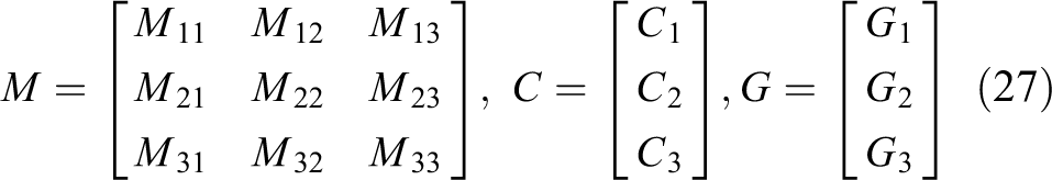
Nonlinear model of the system in equation (27) can be linearized at the upright position of the pendulums. The dynamics model is rearranged

\ddot{q} = M (q) {F_{i} - C (q, \dot{q}) - G (q)}

State vector of the RDIP system consists of six states

q = {[\emptyset_{A}, {\dot{\emptyset}}_{A}, \emptyset_{I}, {\dot{\emptyset}}_{I}, \emptyset_{O}, {\dot{\emptyset}}_{O}]}^{T} = {[x_{1}, x_{2}, x_{3}, x_{4}, x_{5}, x_{6}]}^{T}

The system model is linearized using small angle approximation

cos \emptyset_{I} \approx 1, cos \emptyset_{O} \approx 1, sin \emptyset_{I} \approx \emptyset_{I}, sin \emptyset_{O} \approx \emptyset_{O}, \emptyset_{I}^{2} = 0, \emptyset_{O}^{2} = 0

The linearized model at the upright position is obtained as

{\begin{matrix} \dot{x} = A x + B u \\ y = C x + D u \end{matrix}

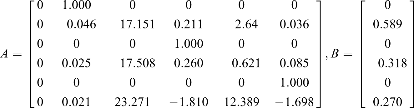
Parameters in Tables 3 and 4 are substituted into the state space model expressed by equation (29).

State matrix (A) and input matrix (B) become as follows

A = [\begin{matrix} 0 & 1.000 & 0 & 0 & 0 & 0 \\ 0 & - 0.046 & - 17.151 & 0.211 & - 2.64 & 0.036 \\ 0 & 0 & 0 & 1.000 & 0 & 0 \\ 0 & 0.025 & - 17.508 & 0.260 & - 0.621 & 0.085 \\ 0 & 0 & 0 & 0 & 0 & 1.000 \\ 0 & 0.021 & 23.271 & - 1.810 & 12.389 & - 1.698 \end{matrix}], B = [\begin{matrix} 0 \\ 0.589 \\ 0 \\ - 0.318 \\ 0 \\ 0.270 \end{matrix}]

Controller design

LQR controller

LQR is an optimal controller. The optimal controller controls the system at the minimum cost.

Cost function of LQR is expressed by

J = \int_{0}^{\infty} (x^{T} Q x + u^{T} R u) d t

where Q is state weighting matrix and R is input weighting matrix.

The following algebraic Riccati equation is used to determine the covariance matrix, P.

A^{T} P + P A + Q - P B R^{- 1} B^{T} P = 0

The controller gain, K, is determined by using $K = R^{- 1} B^{T} P$ . LQR is applied to control the RDIP system in order to see the performance in comparison to the proposed mixed sensitivity H∞ controller.

Mixed sensitivity H∞ controller

Mixed sensitivity of S/KS/T H∞ controller is proposed to balance the RDIP system. In this mixed sensitivity controller, three closed loop transfer functions in equation (32) are shaped by using H∞ optimization to achieve the desired performance

{\begin{array}{l} S (s) = {[1 + G_{N} (s) K (s)]}^{- 1} \\ T (s) = G_{N} (s) K (s) {[1 + G_{N} (s) K (s)]}^{- 1} = K (s) G_{N} (s) S (s) \\ K (s) S (s) = K (s) {[1 + G_{N} (s) K (s)]}^{- 1} \end{array}

where $S (s), T (s)$ , and $K (s) S (s)$ are known as sensitivity function, complementary sensitivity function, and output control sensitivity function, respectively. K(s) is controller transfer function. Good tracking performance and reduction of overshoot requires S(s) to be small while robust stability with multiplicative output uncertainties and noise attenuation requires T(s) to be small. However, since

S (s) + T (s) = 1

Therefore, the requirements cannot be fulfilled simultaneously at all frequency range. Normally, good tracking performance and overshoot reduction are required at low frequency range, noise attenuation and robust stability are required at high frequency range.

Therefore, the controller can be designed with small S(s) at low frequency and small T(s) at high frequency as per the desired control performances.

Structure of the mixed sensitivity of S/KS/T H∞ controller of the RDIP system is shown in Figure 7. In order to achieve the desired performance of the robust controller, three weighting functions $(W_{e}, W_{u}, W_{p})$ are designed. The error signal, v, the control input, u, and the output of the system, $G_{N} u$ , are weighted by W_e , W_u , and W_p , respectively. Equivalent representation of the mixed sensitivity structure in Figure 7 is presented by Figure 8.

Figure 7.

Structure of the mixed sensitivity H∞ controller. The nominal plant and the controller respectively presented by G_N and K. u is known as the control input vector. z ₁, z ₂, and z₃ represent weighted error $(W_{e} v)$ , weighted input $(W_{u} u)$ , and weighted output $(W_{p} G_{N} u)$ , respectively.

Figure 8.

Standard feedback system configuration.

In Figure 8, G_A illustrates the plant G_N augmented with W_e , W_u , and W_p . The plant consists of two inputs and two outputs. $y, u, w$ , and z represent output (including feedback and measured signal), control input, exogenous vector (including disturbances, noises, and reference signal), and performance vector (including all control signals, tracking errors), respectively. The augmented plant, G_A , can be expressed by

[\begin{matrix} z \\ y \end{matrix}] = [\begin{matrix} G_{A 11} & G_{A 12} \\ G_{A 21} & G_{A 22} \end{matrix}] [\begin{matrix} w \\ u \end{matrix}]

where $G_{A * *}$ is the transfer function between inputs and outputs of the augmented plant G_A. From Figure 8, z can be written as

z = [\begin{matrix} z_{e} \\ z_{u} \\ z_{p} \end{matrix}] = [\begin{matrix} W_{e} & - W_{e} G_{N} \\ 0 & W_{u} \\ 0 & W_{p} G_{N} \end{matrix}] [\begin{matrix} w \\ u \end{matrix}]

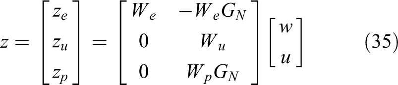
Substitution of all sensitivity functions in equation (32) into the performance signals, $z_{e}, z_{u}, z_{p}$ , results in

N = [\begin{matrix} W_{e} S (s) \\ W_{u} K (s) S (s) \\ W_{p} T (s) \end{matrix}]

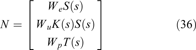
Design objective of the controller is to determine the controller that minimizes the cost function of the system expressed by

\begin{matrix} min \\ k \end{matrix} ∥ N {(K) ∥}_{\infty}

When the cost function is defined as the infinity norm of N

N = {∥ [\begin{matrix} W_{e} S (s) \\ W_{u} K (s) S (s) \\ W_{p} T (s) \end{matrix}] ∥}_{\infty}

Weighting function design

Selection of the weighting functions, W_e , W_u , and W_p , is important in designing the mixed sensitivity H∞ controller. Weighting function W_e is for the sensitivity, S(s). Shaping S(s) improves tracking performance and reduces overshoot of the response. The following diagonal matrix is selected for W_e as expressed in equation (39). Each diagonal element follows equation (40)

W_{e} = diag (W_{e 1}, 0, W_{e 2}, 0, W_{e 3}, 0) = diag (\frac{0.526 s + 60.8}{s + 0.00608}, 0, \frac{0.0475 s + 10}{s + 1}, 0, \frac{0.526 s + 10}{s + 0.1}, 0)

W_{e} = \frac{s / M + ω_{0}}{s + ω_{0} A}

where A, ω₀, and M represent the desired steady state error, bandwidth, and sensitivity peak, respectively.

Frequency response of the inverse of W_e is shown in Figure 9. The figure shows that the magnitudes of $W_{e 1}^{- 1}$ , $W_{e 2}^{- 1}$ , and $W_{e 3}^{- 1}$ are very small at low frequency range and large at high frequency range which make good tracking performance and reduce overshoot of the response, respectively.

Figure 9.

Frequency response of the inverse of sensitivity weighting functions.

The system dynamics model is always not exactly the same as the actual system. The difference is called model uncertainty. The model uncertainty is expressed by

G_{UN} (s) = G_{N} (s) (1 + Δ (s))

where G_N(s) represents nominal model. Δ(s) is model uncertainty. Frequency responses of arm, inner pendulum, and outer pendulum with model uncertainties are shown in Figure 10(a) to (c).

Figure 10.

Frequency responses of the nominal model and the perturbed system: (a) arm, (b) inner pendulum, and (c) outer pendulum.

System perturbation is determined from

Δ (s) = \frac{G_{UN} (s) - G_{N} (s)}{G_{N} (s)}

In order to design a robust controller to achieve the desired performance, the complementary sensitivity function has to satisfy

\bar{σ} (Δ (s)) < \bar{σ} (W_{e} (s))

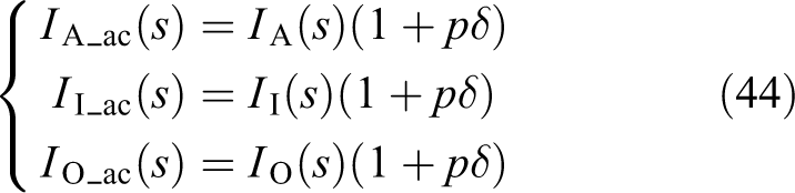
To evaluate robustness of the controllers, variation of moments of inertia of the arm and both pendulums $(I_{A}, I_{I}$ , and $I_{O})$ are selected to simulate parametric uncertainties. These parameters are varied from −10% to +10% from their nominal values. Thus, the actual values of the moments of inertia of the arm, the inner and the outer pendulums are expressed by

{\begin{array}{l} I_{A_ac} (s) = I_{A} (s) (1 + p δ) \\ I_{I_ac} (s) = I_{I} (s) (1 + p δ) \\ I_{O_ac} (s) = I_{O} (s) (1 + p δ) \end{array}

where $P = 0.1, - 1 \leq δ \leq 1$ .

Shaping T(s) is desirable for noise attenuation and for robust stability with respect to multiplicative output uncertainty. Stability of the closed loop system with variation of the model parameters and measured noise attenuation are ensured by W_P .

The following diagonal matrix is selected for W_P .

W_{p} = diag (W_{p 1}, 0, W_{p 2}, 0, W_{p 3}, 0) = diag (\frac{1.1 s + 0.43}{s + 21.5}, 0, \frac{s + 0.02}{s + 0.02}, 0, \frac{s + 3.448}{0.01 s + 0.5}, 0)

W_{e} = \frac{s + ω_{0} / M}{A s + ω_{0}}

Each diagonal element follows equation (46).

Frequency responses of the inverse of the selected complementary sensitivity weighting functions are shown in Figure 11. The figure shows that the magnitudes of $W_{p 1}^{- 1}$ , $W_{p 2}^{- 1}$ , and $W_{p 3}^{- 1}$ are high at low frequency range and small at high frequency range which make noise attenuation and robust stability. In Figure 12, the model uncertainties are depicted together with the respective complementary sensitivity weighting functions.

Figure 11.

Frequency response of the inverse of complementary sensitivity weighting functions.

Figure 12.

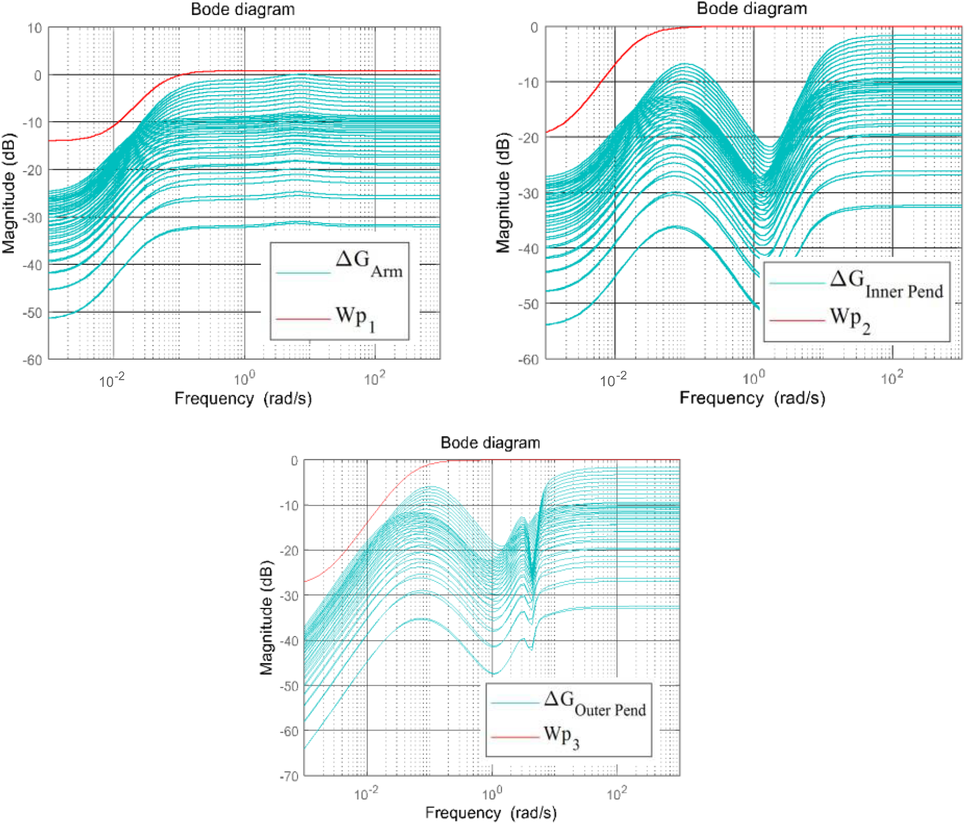
The system uncertainties and the complementary sensitivity weighting functions.

It can be seen that all the uncertainties, Δ(s), are below the respective weighting functions. Hence, the selected weighting functions satisfy equation (43).

W_u is the weighting function of $K (s) S (s)$ that defines control signal characteristics. Normally, a constant value or a high pass filter is selected for W_u . The following constant matrix is used for this system

W_{u} = [1]

Simulation and experimental results

This section shows simulation and experimental results of the mixed sensitivity H∞ controller in comparison with LQR. To find optimal gain, K_LQR, of LQR, the state weighting matrix, Q, and the input weighting matrix, R, are selected as follows

Q = diag (1, 0, 100, 0, 100, 0), R = [1]

In the RDIP system, the most important states are angles of the inner and the outer pendulums. Therefore, weights of these states are set to high values than the other states. With these weighting matrices, angles of the inner and the outer pendulums are equally weighted. Based on the selected weighting matrices, the optimal gain of LQR is obtained as follows.

K_{LQR} = [1.000, 1.300, 861.8, 181.6, 10, 49.2, 240.5]

In the mixed sensitivity H∞ controller, weighting functions are defined as explained in weighting functions design session and the state space model of the system in equation (29) are used. The controller K is obtained as follows

K = [K_{1}, K_{2}, K_{3}, K_{4}, K_{5}, K_{6}]

where $K_{1}, K_{2}, K_{3}, K_{4}, K_{5}, K_{6}$ are obtained as expressed in equation (51)

\begin{array}{l} K_{1} = \frac{4.82 exp 10 s^{11} + 6.57 exp 11 s^{10} + 4.16 exp 12 s^{9} + 1.68 exp 13 s^{8} + 3.68 exp 13 s^{7} + 2.91 exp 13 s^{6} + 6.01 exp 12 s^{5} + 5.29 exp 11 s^{4} + 2.26 exp 10 s^{3} + 4.56 exp 8 s^{2} + 3.25 exp 6 s - 3515}{s^{12} + 1.06 exp 5 s^{11} - 5.52 exp 11 s^{10} - 0.30 exp 12 s^{9} - 1.98 exp 13 s^{8} - 4.13 exp 13 s^{7} - 6.47 exp 13 s^{6} - 4.63 exp 13 s^{5} - 8.48 exp 12 s^{4} - 6.23 exp 11 s^{3} - 2.07 exp 10 s^{2} - 2.67 exp 8 s - 1.000 exp 6} \\ K_{2} = \frac{4.51 exp 10 s^{11} + 3.41 exp 11 s^{10} + 1.75 exp 12 s^{9} + 8.30 exp 12 s^{8} + 8.57 exp 12 s^{7} + 1.89 exp 12 s^{6} + 1.77 exp 11 s^{5} + 8.33 exp 9 s^{4} + 2.0 exp 8 s^{3} + 2.33 exp 6 s^{2} + 1.0 exp 4 s + 13.66}{s^{12} + 1.06 exp 5 s^{11} - 5.52 exp 11 s^{10} - 0.30 exp 12 s^{9} - 1.98 exp 13 s^{8} - 4.13 exp 13 s^{7} - 6.47 exp 13 s^{6} - 4.63 exp 13 s^{5} - 8.48 exp 12 s^{4} - 6.23 exp 11 s^{3} - 2.07 exp 10 s^{2} - 2.67 exp 8 s - 1.000 exp 6} \\ K_{3} = \frac{8.61 exp 9 s^{11} + 3.48 exp 10 s^{10} - 1.25 exp 10 s^{9} + 4.03 exp 11 s^{8} + 5.58 exp 11 s^{7} + 1.29 exp 11 s^{6} + 1.22 exp 10 s^{5} + 5.72 exp 8 s^{4} + 1.36 exp 7 s^{3} + 1.497 exp 5 s^{2} + 573.6 exp 6 s - 0.3228}{s^{12} + 1.06 exp 5 s^{11} - 5.52 exp 11 s^{10} - 0.30 exp 12 s^{9} - 1.98 exp 13 s^{8} - 4.13 exp 13 s^{7} - 6.47 exp 13 s^{6} - 4.63 exp 13 s^{5} - 8.48 exp 12 s^{4} - 6.23 exp 11 s^{3} - 2.07 exp 10 s^{2} - 2.67 exp 8 s - 1.000 exp 6} \\ K_{4} = \frac{9.07 exp 10 s^{11} + 8.18 exp 11 s^{10} - 2.923 exp 12 s^{9} + 7.533 exp 12 s^{8} + 6.654 exp 12 s^{7} + 1.432 exp 12 s^{6} + 1.319 exp 11 s^{5} + 6.006 exp 9 s^{4} + 1.35 exp 8 s^{3} + 1.268 exp 6 s^{2} + 1853 s - 12.45}{s^{12} + 1.06 exp 5 s^{11} - 5.52 exp 11 s^{10} - 0.30 exp 12 s^{9} - 1.98 exp 13 s^{8} - 4.13 exp 13 s^{7} - 6.47 exp 13 s^{6} - 4.63 exp 13 s^{5} - 8.48 exp 12 s^{4} - 6.23 exp 11 s^{3} - 2.07 exp 10 s^{2} - 2.67 exp 8 s - 1.000 exp 6} \\ K_{5} = \frac{7.57 exp 10 s^{11} + 2.33 exp 12 s^{10} + 1.99 exp 13 s^{9} + 6.07 exp 13 s^{8} + 5.31 exp 13 s^{7} + 1.09 exp 13 s^{6} + 9.66 exp 11 s^{5} + 4.34 exp 10 s^{4} + 9.95 exp 8 s^{3} + 1.05 exp 7 s^{2} + 3.59 exp 4 s + 2.242}{s^{12} + 1.06 exp 5 s^{11} - 5.52 exp 11 s^{10} - 0.30 exp 12 s^{9} - 1.98 exp 13 s^{8} - 4.13 exp 13 s^{7} - 6.47 exp 13 s^{6} - 4.63 exp 13 s^{5} - 8.48 exp 12 s^{4} - 6.23 exp 11 s^{3} - 2.07 exp 10 s^{2} - 2.67 exp 8 s - 1.000 exp 6} \\ K_{6} = \frac{- 1.23 exp 12 s^{11} - 1.28 exp 13 s^{10} - 3.15 exp 13 s^{9} + 1.80 exp 13 s^{8} + 4.87 exp 13 s^{7} + 1.18 exp 13 s^{6} + 1.13 exp 12 s^{5} + 5.38 exp 10 s^{4} + 1.29 exp 9 s^{3} + 1.45 exp 7 s^{2} + 5.94 exp 4 s - 50.52}{s^{12} + 1.06 exp 5 s^{11} - 5.52 exp 11 s^{10} - 0.30 exp 12 s^{9} - 1.98 exp 13 s^{8} - 4.13 exp 13 s^{7} - 6.47 exp 13 s^{6} - 4.63 exp 13 s^{5} - 8.48 exp 12 s^{4} - 6.23 exp 11 s^{3} - 2.07 exp 10 s^{2} - 2.67 exp 8 s - 1.000 exp 6} \end{array}

Simulation results

Balancing performance of the nominal RDIP system using the mixed sensitivity H∞ controller and LQR is shown in Figures 13 and 14. The initial states are set at $x (0) = {[0 0 0.022 0 0 0]}^{T}$ . Figure 13 shows the comparison of time domain responses of the inner pendulum from both controllers while Figure 14 shows the comparison of the outer pendulum.

Figure 13.

Time domain responses of inner pendulum (nominal).

Figure 14.

Time domain responses of outer pendulum (nominal).

As shown in Figures 13 and 14, the settling time of the inner and the outer pendulums using LQR is only around 97% and 94% of the mixed sensitivity H∞ controller, respectively. The peak value of the inner and the outer pendulums using LQR is only around 33% and 29% of the mixed sensitivity H∞ controller, respectively.

Even though both controllers have similar settling time, the other performances on the nominal plant using LQR are better than the mixed sensitivity H∞ controller. The results prove that both the mixed sensitivity H∞ controller and LQR can balance both inner and outer pendulums under nominal condition. However, LQR has better control performance than the mixed sensitivity H∞ controller on the nominal system.

Uncertainty from parameter variation

In order to evaluate robustness of the controllers, moments of inertia of the arm and the pendulums are varied from their nominal values for ±10%. Step response comparison of the arm with moment of inertia variation is shown in Figures 15 and 16.

Figure 15.

Step response of the arm using LQR under uncertainty. LQR: linear quadratic regulator.

Figure 16.

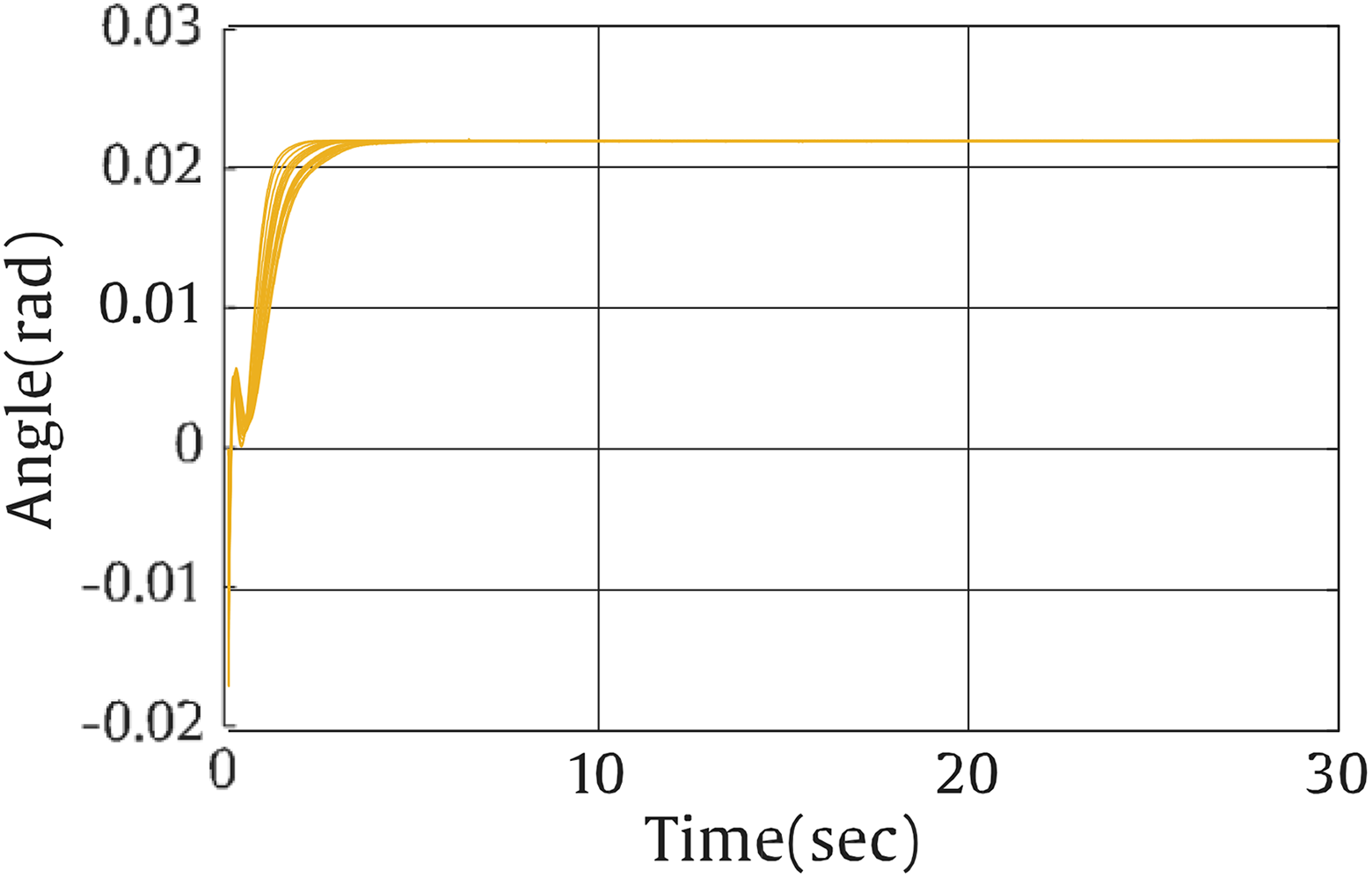
Step response of the arm using the mixed sensitivity H∞ controller under uncertainty.

The results show that settling time and rise time of the proposed controller is less than LQR. There is no overshoot in the proposed controller. The proposed mixed sensitivity H∞ controller gives better performance than LQR under parameter variation.

In order to further confirm the control performance, step response comparison of the arm at the minimum (case 1) and the maximum (case 2) moments of inertia are considered. Figure 17(a) and (b) shows the comparison of step response obtained from both controllers at the minimum (case 1) and maximum (case 2) moments of inertia.

Figure 17.

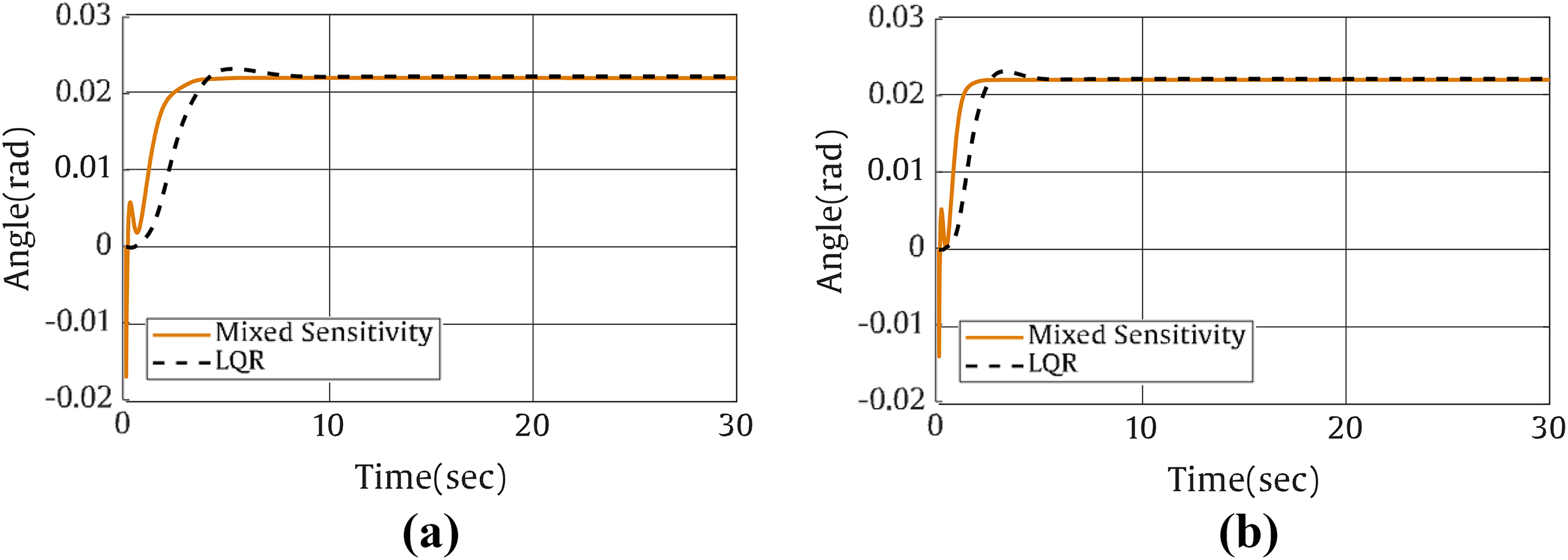
Step response comparison of the arm at (a) minimum and (b) maximum moments of inertia.

In this simulation, the following values are applied

{\begin{array}{l} (Nominal (I_{A}) = 0.023584, Max (I_{A}) = 0.025942, Min (I_{A}) = 0.021225) \\ (Nominal (I_{I}) = 0.01606, Max (I_{I}) = 0.017666, Min (I_{I}) = 0.014454) \\ (Nominal (I_{O}) = 0.02262, Max (I_{O}) = 0.020358, Min (I_{O}) = 0.024882) \end{array}

where $Max (I_{*}) = Nominal (I_{*}) + 0.1 × Nominal (I_{*})$ and $Min (I_{*}) = Nominal (I_{*}) - 0.1 × Nominal (I_{*})$ .

Subscript A, I, and O represent arm, inner, and outer pendulum. It is clearly seen that the proposed mixed sensitivity H∞ controller can stabilize the system without overshoot and shorter settling time than LQR at both case 1 and case 2.

Disturbance rejection

In order to evaluate disturbance rejection performance of the proposed controller, a perturbation with 0.0349 rad amplitude is applied on the inner pendulum and the outer pendulum at the 10th second. Figures 18 and 19 show disturbance rejection performance of the system when the inner and outer pendulums are disturbed.

Figure 18.

Time response of (a) inner pendulum and (b) outer pendulum when inner pendulum is perturbed.

Figure 19.

Time response of (a) inner pendulum and (b) outer pendulum when outer pendulum is perturbed.

The results show that after the deviation from the upright position of both pendulums for some period of time, both controllers re-stabilize the system. However, the time domain performances of the proposed controller, such as settling time, peak value, and rise time, are shorter than LQR as summarized in Table 5.

Table 5.

Comparison of the time domain performance specification for disturbance rejection.

Performance specification	Controller	When inner pend: perturbed		When outer pend: perturbed
Performance specification	Controller	Inner pend	Outer pend	Inner pend	Outer pend
Rise time (s)	LQR Mixed sensitivity	3.0339E−4 1.4090E−7	2.6317E−4 1.3746E−7	3.0339E−4 6.7733E−7	2.6317E−4 6.0057E−7
Settling time (s)	LQR	15.0543	15.1023	15.0543	15.1023
	Mixed sensitivity	12.8356	12.8604	13.7185	13.7556
Peak (rad)	LQRMixed sensitivity	0.00550.0013	0.00400.0011	0.09480.0092	0.06790.0080
Peak time (s)	LQR	11.1590	11.2460	11.1590	11.2460
	Mixed sensitivity	10.0190	10.0180	10.0640	10.3240

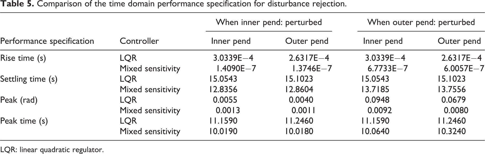
LQR: linear quadratic regulator.

The results show that peak value of the inner and the outer pendulums of the mixed sensitivity H∞ controller are only 23% and 27.5% of LQR when the inner pendulum is perturbed and only 9.7% and 11% when the outer pendulum is perturbed. It clearly proves that all time domain performances of the mixed sensitivity H∞ controller are better than LQR under perturbation.

Tracking performance

In order to evaluate tracking performance of the RDIP system, various steps reference trajectory is applied. Tracking performance of the proposed controller is shown in Figure 20. From the result, the arm can track the reference trajectory without overshoots while balancing both pendulums using the proposed controller.

Figure 20.

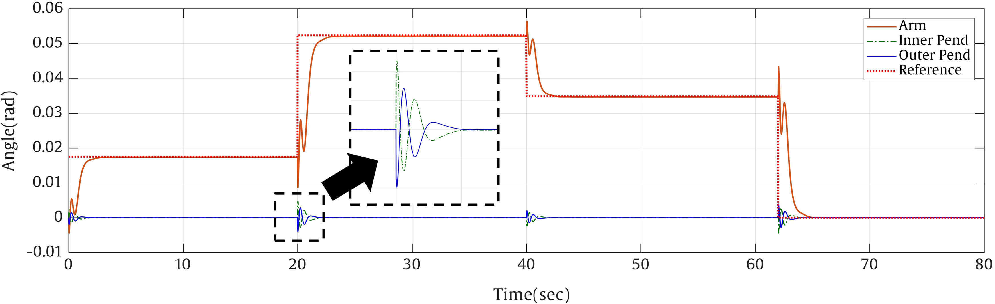
Response of the system in tracking the reference step trajectory of the arm using the proposed controller.

Experimental results

In order to verify the robustness of the proposed controller, several experiments are conducted on the developed RDIP system. USB to TTL module based on CH340 chip is used in collecting experimental data from the system. Figures 21 and 22 illustrate balancing performance on the nominal system using LQR and the proposed mixed sensitivity H∞ controller, respectively.

Figure 21.

Balancing performance on the nominal system using LQR. LQR: linear quadratic regulator.

Figure 22.

Balancing performance on the nominal system using the proposed controller.

The experimental results show that both pendulum angles fluctuate around ±0.01 rad. Even though the pendulum angles fluctuate, both controllers are able to stabilize the system. The experimental results show that the inner and outer pendulums can be balanced at the upright position by using both controllers at the nominal condition.

To evaluate disturbance rejection performance, a disturbance is applied to the inner pendulum. The disturbance force makes a change of pendulum angle. Figure 23 shows experimental result of pendulum angles using LQR under disturbance. From the result, LQR cannot stabilize the system under the disturbance.

Figure 23.

Experimental results of the pendulum angles under disturbance using LQR. LQR: linear quadratic regulator.

Figure 24 shows experimental result of the system using the proposed mixed sensitivity H∞ controller under disturbance. From the result, responses of both pendulums oscillate due to the applied disturbance force; however, the proposed mixed sensitivity controller is able to stabilize both pendulums to the upright position within short time period.

Figure 24.

Experimental results of the pendulum angles under disturbance using the proposed controller.

The system states deviation due to applied several impulse disturbances are shown in Figure 25. The control input is shown in Figure 26. From the result, the control input fluctuates with the applied disturbances. However, it is still within the supplied capacity. Snapshots from the balancing experiment of RDIP system are shown in Figure 27.

Figure 25.

Experimental results of both pendulums and arm under disturbance using mixed sensitivity H∞ controller.

Figure 26.

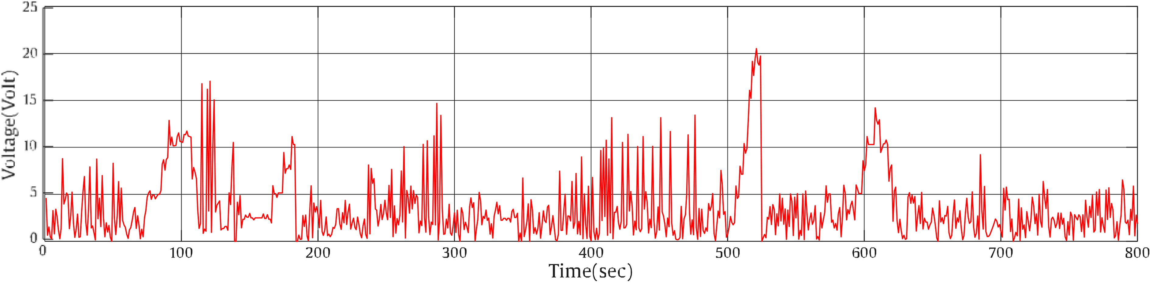
Control input of the system.

Figure 27.

Snapshots from balancing experiment of RDIP system. RDIP: rotary double inverted pendulum.

Conclusion

Mixed sensitivity of S/KS/T H∞ controller was proposed to balance a RDIP system. The real RDIP system was built as per design. Hardware of the system was realized and explained in detail. The RDIP system was driven by a DC motor at the rotating arm. STM32F407 microcontroller was selected as the controller of the system. Dynamic model of the system was derived using Lagrange equation of motion. Mixed sensitivity control synthesis and weighing functions selection were presented. The proposed mixed sensitivity H∞ controller was applied to control the RDIP system. The proposed mixed sensitivity H∞ controller was evaluated in comparison with LQR by both simulation and experiment. In the simulation, balancing performance on the nominal system, tracking performance, disturbance rejection, and robustness performance under uncertainty were considered. Experiments were conducted to prove the results from the simulation. Even though the pendulum angles fluctuated around the upright position with small variation, both controllers could stabilize the nominal system. However, it was observed that transient response of the nominal system using LQR was better than the proposed controller. However, the proposed mixed sensitivity H∞ controller showed better performance than LQR with the presence of disturbances and uncertainties. LQR could not stabilize the RDIP system under the disturbance while the proposed mixed sensitivity H∞ controller could successfully control the RDIP system.

Footnotes

Declaration of conflicting interests

The author(s) declared no potential conflicts of interest with respect to the research, authorship, and/or publication of this article.

Funding

The author(s) received no financial support for the research, authorship, and/or publication of this article.

ORCID iD

Sondarangallage DA Sanjeewa

References

Siuka

Schöberl

. Applications of energy based control methods for the inverted pendulum on a cart. Rob Auton Syst 2009; 57(10): 1012–1017.

Linden

Lambrechts

. H∞ control of an experimental inverted pendulum with dry friction. In: Proceedings of the First IEEE conference on control applications, Dayton, OH, 13–16 September 1992, pp. 123–128.

Cheang

Chen

. Stabilizing control of an inverted pendulum system based on H∞ loop shaping design procedure. In: Proceedings of the 3rd World Congress on intelligent control and automation, Hefei, 28 June–2 July 2000, vol. 5, pp. 3385–3388.

Graichen

Treuer

Zeitz

. Swing-up of the double pendulum on a cart by feedforward and feedback control with experimental validation. Brief paper Automatica 2007; 43(1): 63–71.

Liu

Zhou

. Static H∞ loop shaping real-time control of a double inverted pendulum system. In: International conference on automation and logistics, Shenyang, China, 5–7 August 2009, pp. 670–674.

Tsai

. Application of model predictive control to parallel-type double inverted pendulum driven by a linear motor. In: IECON. 33rd annual conference of the IEEE Industrial Electronics Society, Taipei, 5–8 November 2007, pp. 2904–2909.

Kurode

Shailaja

Chalanga

Asif

Bandyopadhyay

. Swing-up and stabilization of rotary inverted pendulum using sliding mode. In: Proceedings of the 18th World Congress, The International Federation of Automatic Control, Milano, Italy, 28 August–2 September 2011, pp. 10685–10690.

Sukontanakarn

Parnichkun

. Real-time optimal control for rotary inverted pendulum. Am J Appl Sci 2009; 6(6): 1106–1115.

Pakdeepattarakorn

Thamvechvitee

Songsiri

. Dynamic models of a rotary double inverted pendulum system. 2004 IEEE Region 10 Conference TENCON 2004; 4: 558–561.

10.

Komine

Iwase

Suzuki

. Rotational control of double pendulum. In: Proceedings of the IFAC mechatronic systems, Sydney, Australia, 6–8 September 2004, pp. 325–330.

11.

Pan

Xue

Chen

. Design and implementation of rotary inverted pendulum motion control hardware-in-the-loop simulation platform. In: Proceedings of IEEE conference on decision and control, Xuzhou, 26–28 May 2010, pp. 2328–2333.

12.

Casanova

Salt

Piza

. Controlling the double rotary inverted pendulum with multiple feedback delays. Int J Comput Commun Cont 2012; 7(1): 20–38.

13.

Jiang

Tian

Zhang

. Robust quadratic stabilizability and H∞ control of uncertain linear discrete-time stochastic systems with state delay. Math Probl Eng 2016.

14.

Tuvayanond

Parnichkun

. Position control of a pneumatic surgical robot using PSO based 2-DOF H∞ loop shaping structured controller. Mechatronics 2017; 43: 40–55.

15.

Zames

. Model reference transformations, multiplicative semi norms, and approximate inverses. IEEE Trans Autom Control 1982; 26(2): 301–320.

16.

Doyle

Glover

Khargonekar

. State-space solutions to standard H2 and H∞ control problems. IEEE Trans Autom Control 1989; 34(8): 831–847.

17.

McFarlane

Glover

. A loop-shaping design procedure using H∞ synthesis. IEEE Trans Auto Control 1992; 37(6): 759–769.

18.

Kwakernaak

. Mixed sensitivity design. In: Submitted for presentation during the 15th proceedings of IFAC World Congress, Barcelona, Spain, 21–26 July 2002, pp. 21–26.

19.

Yuan

Long

. Research for the clamping force control of pneumatic manipulator based on the mixed sensitivity method. Procedia Eng 2012; 31: 1225–1233.

20.

Rachedi

Hemici

Bouri

. Design of an H∞ controller for the Delta robot: experimental results. Adv Robotics 2015; 29(18): 1165–1181.

21.

You

Chen

. Tracking control research of high-order flexible structures on the H-infinity control method. In: 2010 2nd International Conference on Advanced Computer Control, Shenyang, 27–29 March 2010, pp. 111–115.

22.

Ozana

Stepan

Vojcinak

Petr

Pies

Martin

. Mixed Sensitivity H-∞ control for helicopter model. In: 12th IFAC conference on programmable devices and embedded systems, Velke Karlovice, September 2013, pp. 25–27. Czech Republic: The International Federation of Automatic Control.

23.

Bao

Xinping

Zhenyu

. Rudder based roll control via host-computer of a robotic boat. Int J Adv Robotic Sys 2009; 6(1): p6773.

24.

Alfaya

Guillermo

Manuel

. Controllability analysis and robust control of a one-stage refrigeration system. Eur J Control 2015; 26: 53–62.

25.

Bejarano

Guillermo

Alfaya

Manuel

. Multivariable analysis and H∞ control of a one-stage refrigeration cycle. Applied Thermal Engineering 2015; 91(5): 1156–1167.

26.

Delettre

Laurent

Haddab

. Robust control of a planar manipulator for flexible and contactless handling. Mechatronics 2012; 22(6): 852–861.

27.

Iannino

Colla

Innocenti

. Design of a H∞ Robust controller with µ-analysis for steam turbine power generation applications. Energies 2017; 10: 1026.

28.

Fragoso

Garrido

Vázquez

. Comparative analysis of decoupling control methodologies and H∞ multivariable robust control for variable-speed, variable-pitch wind turbines: app lab-scale wind turbine. Sustainability 2017; 9: 713.

Control of rotary double inverted pendulum system using mixed sensitivity H∞ controller

Abstract

Keywords

Introduction

System architecture

Dynamic model

DC motor model

Nonlinear dynamic model

Controller design

LQR controller

Mixed sensitivity H∞ controller

Weighting function design

Simulation and experimental results

Simulation results

Uncertainty from parameter variation

Disturbance rejection

Tracking performance

Experimental results

Conclusion

Footnotes

Declaration of conflicting interests

Funding

ORCID iD

References