Sage Journals: Discover world-class research

Abstract

Global positioning system signal does not penetrate into the water volume, and autonomous underwater vehicle have to use the inertial navigation system that will cause an inevitable cumulative error. Terrain reference position can zero out the inertial navigation system error and have been widely used. To improve the positioning accuracy, the planning path of the underwater robot is required to pass through the suitable matching areas in the path planning stage. So, a gridding map is needed to quantify the suitability of the terrain and to partition the suitable matching area and the unsuitable matching area optimally. In this article, we will focus on the quantitative method of terrain suitability and the grid parameter solution method for optimal partition of suitable matching area. Finally, the validity of the algorithm is obtained using the ship borne data. The results show that in the low suitability blocks, the influence of measurement error on terrain reference position accuracy is higher than that in high suitability blocks. And the average of terrain reference position deviation obtained of the path passed through the high suitability area is 53.3% which is lower than that of the path passed through the low suitability area, and the standard deviation of the position deviation is reduced by 21.15%.

Keywords

Autonomous underwater vehicle terrain reference position terrain suitable analysis optimal partition of suitable matching area map gridding

Introduction

Terrain reference navigation (TRN) is an ideal aided navigation method that has no time accumulation error. At present, underwater TRN technology uses multi-beam as the measurement equipment, which improves both acquisition speed and matching accuracy.^1,2 However, there are some disadvantages associated with TRN, such as large errors in terrain measurement, fewer terrain features, and the lower acquisition speed of the measurement data, which always cause large position deviation.¹ At present, the research on improving the TRN/terrain reference position (TRP) accuracy mainly focuses on the filtering algorithm, including particle filter (PF),^1,3

–6 robust filtering algorithm,^7,8
–10 point mass filter (PMF),^5,11,12 and so on. The latest research progress on TRN can be referred to the review article.^13

–17 Another way is to improve the positioning accuracy from the perspective of path planning, allowing autonomous underwater vehicle (AUV) to go through the terrain with high adaptability. As shown in Figure 1(a), the error of the reference navigation system exceeds the threshold at the position C and the TRP is needed to correct the navigation error when the AUV navigation is from A to B. If AUV can independently quantify the adaptability of the digital elevation map (DEM) and identification of suitable areas and unsuitable area. Then AUV will be able to obtain a suitability map (Figure 1(b)) to plan a path through a high suitable area (blue route in Figure 1(b)), so that the positioning error at the end of the navigation point will be in a small range. Otherwise, AUV may not reach the target point B through the low suitable area (green route in Figure 1(b)). To make AUV use the topographic map path planning and correct navigation error, the first problem that needs to be solved is to quantify the suitability of the terrain and the problem of the division of the suitable area and the unsuitable area. Now, the TRN path planning method mainly focuses on the path search algorithm. For example, the waypoints selected are based on the binary-tree search algorithm,¹⁸ and the terrain matching navigation method based on the A*.^19
–21 It is worth noting that the key to TRN path planning include two prerequisites: (1) suitability quantization and (2) division of suitable area and unsuitable area. Therefore, this study is mainly to solve these two problems. Because large number of path planning algorithms are based on grid map.^19,21,22 So, the suitable area and the unsuitable area partition are based on topographic gridding. In this article, a method of quantization of terrain suitability and optimal partition of terrain suitability is mainly studied. Based on the DEM gridding, the suitable area and the unsuitable area can be partitioned off optimally.

Figure 1.

Terrain suitability quantification and suitable area partition can realize AUV navigation mode decision and TRN path planning autonomously. AUV: autonomous underwater vehicle; TRN: terrain reference navigation.

There are many quantization methods for terrain suitability^21,22 that is based on terrain height standard deviations. But terrain height standard deviation is not the only factor affecting the suitability. In the following, we will also deduce another important influence factor of terrain suitability, direction, and a more reliable method of suitability quantification is obtained and part the suitable and unsuitable area with gridding method. The size of the mesh of gridding map will affect the suitability of the subblocks. The DEM has been gridded optimally when the suitable area and the unsuitable area are parted into different subblocks to the maximum extent at a certain value of subblock size. In this article, we primarily study parameterized representation methods of terrain suitability and then propose the optimal partition methods for the terrain suitability area based on the grid premise.

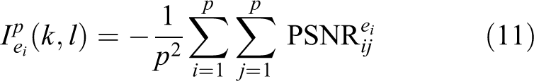
The following research contents of the article include the following parts. In second section, the influence factors and the quantitative evaluation method of TRP accuracy are analyzed. At last, the quantization parameter signal-to-noise ratio (SNR) of the local terrain area is defined. In the third section, the suitability matrix SNR $p$ of one DEM with arbitrary size of subblock is studied. Then, the algorithm for calculating the optimal partition number of any DEM is derived, and a demonstration has shown the process of optimal partition algorithm using the real underwater terrain map. Fourth section is the simulation experiment part, where three different terrain quantization methods (topographic entropy, terrain roughness, SNR) have been compared, and the result shows that SNR has obvious advantages in describing terrain suitability when there is a significant difference of terrain gradients in different directions. In the “Comparison of commonly quantitative parameters” section, the comparison of the positioning accuracy of the high suitable blocks and the low suitable blocks under different measurement errors shows that the positioning accuracy of the low suitable blocks are more easily affected by the measurement error. In the “Accuracy comparison between different suitability paths” section, the TRP accuracy comparison experiment of two path across the low suitability blocks and high suitability blocks, respectively, shows that a higher positioning accuracy and stability can be obtained for a path across the high suitability blocks. Fifth section is the conclusion and future research plan.

Suitability and TRP Accuracy

Influencing factors on TRP accuracy

Suppose AUV has obtained measurement terrain map (MTM) $(x_{i}, x_{j}, z_{i j}), i = 1, 2... m; j = 1, 2... n$ at the current navigation position $(x_{a}, x_{a})$ . The MTM interpolation sequence in the DEM is $h_{i j} (x_{i}, x_{j})$ . In fact, the TRP is used to find the location of the MTM in the DEM. We use distance as a similarity evaluation index and assume that the measurement error for terrain node $(i, j)$ is $ε_{i j}$ . Then, the similarity function can be written as equation (1)

L = \sum_{i = 1}^{m} \sum_{j = 1}^{n} \frac{1}{σ_{i j}^{2}} {(z_{i j} - h_{i j} (X))}^{2}

In the equation, $h_{i j} (X)$ represents the real height of DEM node $(i, j)$ ; $σ_{i j}$ represents the standard deviation of measurement error node $(i, j)$ ; $m, n$ is the row number and column number of MTM node sequence; the equation (1) can be linearized as equation (2)

L = \sum_{i = 1}^{m} \sum_{j = 1}^{n} \frac{1}{σ_{i j}^{2}} {(ε_{i j} - Δ {\hat{h}}_{i j} (X))}^{2}

In the equation, $Δ {\hat{h}}_{i j} (X)$ represents the height difference between the MTM and the interpolation of the MTM in the DEM. The TRP is a translation searching and matching process. We want to find the position deviation $Δ X$ at which the minimum value of L occurs

\frac{\partial L}{\partial X} = - 2 \sum_{i = 1}^{m} \sum_{j = 1}^{n} \frac{1}{σ_{i j}^{2}} (ε_{i j} - \frac{\partial Δ {\hat{h}}_{i j} (•)}{\partial x_{i j}} Δ X) \frac{\partial Δ {\hat{h}}_{i j} (•)}{\partial x_{i j}} = 0

In the equation, X represents the TRP position; $x_{i j}$ represents position of terrain node $(i, j)$ in MTM, which include two components in x and y directions. We can obtain the equation about $Δ X$

\frac{\sum_{i = 1}^{m} \sum_{j = 1}^{n} \frac{1}{σ_{i j}^{2}} \frac{\partial Δ {\hat{h}}_{i j} (•)}{\partial x_{i j}} ε_{i j}}{\sum_{i = 1}^{m} \sum_{j = 1}^{n} \frac{1}{σ_{i j}^{2}} {(\frac{\partial Δ {\hat{h}}_{i j} (•)}{\partial x_{i j}})}^{2}} = Δ X

Measurement sequence $z_{i j}$ is a constant sequence, so $\partial Δ {\hat{h}}_{i j} (•) / \partial x_{i j} = \partial {\hat{h}}_{i j} (•) / \partial x_{i j}$ , and equation (4) can be written as equation (5)

Δ X = \frac{\sum_{i = 1}^{m} \sum_{j = 1}^{n} \frac{1}{σ_{i j}^{2}} \frac{\partial {\hat{h}}_{i j} (•)}{\partial x_{i j}} ε_{i j}}{\sum_{i = 1}^{m} \sum_{j = 1}^{n} \frac{1}{σ_{i j}^{2}} {(\frac{\partial {\hat{h}}_{i j} (•)}{\partial x_{i j}})}^{2}}

Consider the fact that TRP is a two-dimensional search process and that $\partial {\hat{h}}_{i j} (•) / \partial x_{i j}$ is a two-dimensional gradient vector. The terrain is an anisotropic surface, so $\partial {\hat{h}}_{i j} (•) / \partial x_{i j}$ will also have different values in different directions. From equation (5), we can draw the following conclusions:

TRP accuracy is related to measurement error and local topography gradients;

Increases in the terrain gradient can improve positioning accuracy;

Because the terrain gradients have different values in different directions, TRP accuracy will be different in different directions.

The last conclusion is critical. We can infer that even if the terrain changes drastically, if the gradient in a certain direction is small, it may also cause the TRP results to deteriorate as analyzed in “Terrain suitability quantification” section.

Accuracy evaluation of TRP

The terrain surface is an anisotropic surface. According to estimation theory, we can obtain more information for the positioning point.² A reliability evaluation of TRP can be obtained by calculating the information content at TRP position point (6). According to the conclusion of Nygren,² we assume that the variance of elevation error of terrain nodes are independent and identically distributed $N (0, σ_{}^{2})$ .

I_{e} (X^{t}) = E (- \frac{1}{σ_{​}^{2} I J} \sum_{i = 1}^{I} \sum_{j = 1}^{J} {(\frac{\partial h_{i j} (•)}{\partial e})}^{2})

In this equation, $h_{i j} (•)$ represents the interpolation results at point $(x_{i j}, y_{i j})$ ; $(x_{i j}, y_{i j})$ represents the coordinate of node $(i, j)$ for the terrain surface; $I_{e} (X^{t})$ represents the of the terrain surface; $σ_{}^{2}$ represents the variance of the elevation measurement error of the terrain nodes; e represents the unit direction vector. We must consider the fact that terrain gradient along the various directions is not the same. In equation (6), it is necessary to discretize the process. We will disperse the information for the positioning points in eight directions (as show in Figure 2).

Figure 2.

Eight discrete directions of the location terrain information content.

Discrete the results of equation (6) to get equation (7). The inverse of $I_{e_{i}} (X^{t})$ is called Cramer–Rao Low Bound,² and it can reflect the accuracy of the TRP

I_{e_{i}} (X_{​}^{t}) = - \frac{1}{σ_{​}^{2} m n} \sum_{k = 1}^{m} \sum_{l = 1}^{n} {({\hat{h}}_{k l} (X_{​}^{t}) - {\hat{h}}_{k l} (X_{​}^{t} + d • e_{i}))}^{2}

In the equation, e_i represents the unit direction vector and will have eight values; d represents the distance of two terrain nodes when calculating the degradation of the local terrain. So, equation (7) reflects the accuracy of the TRP.² The greater the $I_{e_{i}} (X_{}^{t})$ , the higher the positioning accuracy is, and it is obvious that the value of this type is affected by the following three factors.

The gradient variation item $({\hat{h}}_{k l} (X_{}^{t}) - {\hat{h}}_{k l} (X_{}^{t} + d • e_{i}))$ and greater value of this item will cause higher TRP accuracy.

The terrain gradient will change with the directions of $e_{i}$ , and this leads to the different TRP accuracy at different direction. So, TRP is anisotropic.

The accuracy of TRP is related to the measurement error. The smaller the measurement error is, the higher the positioning accuracy.

From the above analysis, we get the influence factors and the quantitative evaluation of the positioning accuracy. Then, we get the quantitative function of the local terrain adaptation by further analysis.

Terrain suitability quantification

According to the conclusion of Nygren,² the Cramer–Rao bound of TRP $C_{b}^{e_{i}}$ is expressed as

C_{b}^{e_{i}} = {(I_{e_{i}} (X_{​}^{t}))}^{- 1}

$C_{b}^{e_{i}}$ reflects the lower deviation of the location deviation in the direction $e_{i}$ of TRP,² which reflects the probability distribution of the offset of the terrain matching location; and the smaller the $C_{b}^{e_{i}}$ the smaller will be the probability of the deviation to the direction $e_{i}$ . The equation (8) can reflect the distribution of the offset probability distribution in the direction of $e_{i}$ , and the maximum $I_{e_{i}} (X_{}^{t})$ direction in which the maximum value is the maximum direction of the position offset and the position offset probability. As shown in Figure 3, MTM1 and MTM2, two terrain surfaces are represented with different features in eight directions. Figure 3(a) and (b) are TRP results after a test was repeated 10 times. At the same time, values of $C_{b}^{e_{i}}, i = 1, 2...8$ at the eight directions of MTM1 and MTM2 are shown in Figure 3(a) and (b), respectively. There are different TIC values of MTM1 in different directions, the direction in which the minimum is obtained is shown in the MTM1. MTM2 has similarity terrain characteristics in different direction. Figure 3(a) shows the TRP points in 10 times test of MTM1 and MTM2, respectively, and the $C_{b}^{e_{i}}, i = 1, 2...8$ at eight discrete direction $e_{i}, i = 1, 2...8$ are shown in the polar coordinate system with GPS position as its origin. As we can see, a larger value of $C_{b}^{e_{i}}$ (the smaller value of $I_{e_{i}} (X^{t})$ ) will cause an easier deviation of TRP points.

Figure 3.

The $C_{b}^{e_{i}}$ of MTM1 and MTM2 at eight directions (•) and the TRP points distribution (•) relative to GPS position (•). (a) MTM1, (b) MTM2, (c) $C_{b}^{e_{i}}$ of MTM1 and the TRP points distribution relative to GPS position, and (d) $C_{b}^{e_{i}}$ of MTM2 and the TRP points distribution relative to GPS position. MTM: measurement terrain map; TRP: terrain reference position.

We refer to SNR as the suitability function of TRP, its value is the minimum value of $I_{e_{i}} (X_{}^{t}), i = 1, 2...8$ as shown in equation (9). From its definition, we can see that SNR is a directional parameter. It indicates the maximum probability direction of position deviate to. As we can see in Figure 4, the TRP likelihood function of MTM1 and MTM2 that the descending speed of the likelihood function along the direction of the SNR is very slow. The terrain in this direction of SNR has a strong self-similarity, and it is easy to lead to position deviation

\begin{array}{l} SNR = min (I_{e_{i}} (X_{​}^{t})) \\ = min (- \frac{1}{σ_{​}^{2} m n} \sum_{i = 1}^{I} \sum_{j = 1}^{J} {({\hat{h}}_{i j} (X_{​}^{t}) - {\hat{h}}_{i j} (X_{​}^{t} + d • e_{i}))}^{2}) \end{array}

Figure 4.

The likelihood of MTM1 (a) and MTM2 (b). MTM: measurement terrain map. MTM: measurement terrain map.

Equation (8) can calculate the suitability value of a terrain block with a size of $I \times J$ nodes.

Optimal partition of terrain suitable area

Suitability quantization of DEM under arbitrary gridding

We are concerned with the problem of gridding the DEM with optimal partition of the suitable area and unsuitable area. The next step is to find the optimal partition method for the suitable region and unsuitable region in DEM. Figure 5 shows the division process of a DEM. Figure 5(a) to (d) show the distribution of suitable and unsuitable area during the process of mesh size changes.

Figure 5.

An example of DEM partitioning process. (a) Divide the DEM into four blocks, (b) divide the DEM into nine blocks, (c) divide the DEM into 16 blocks, and (d) divide the DEM into 25 blocks. DEM: digital elevation map.

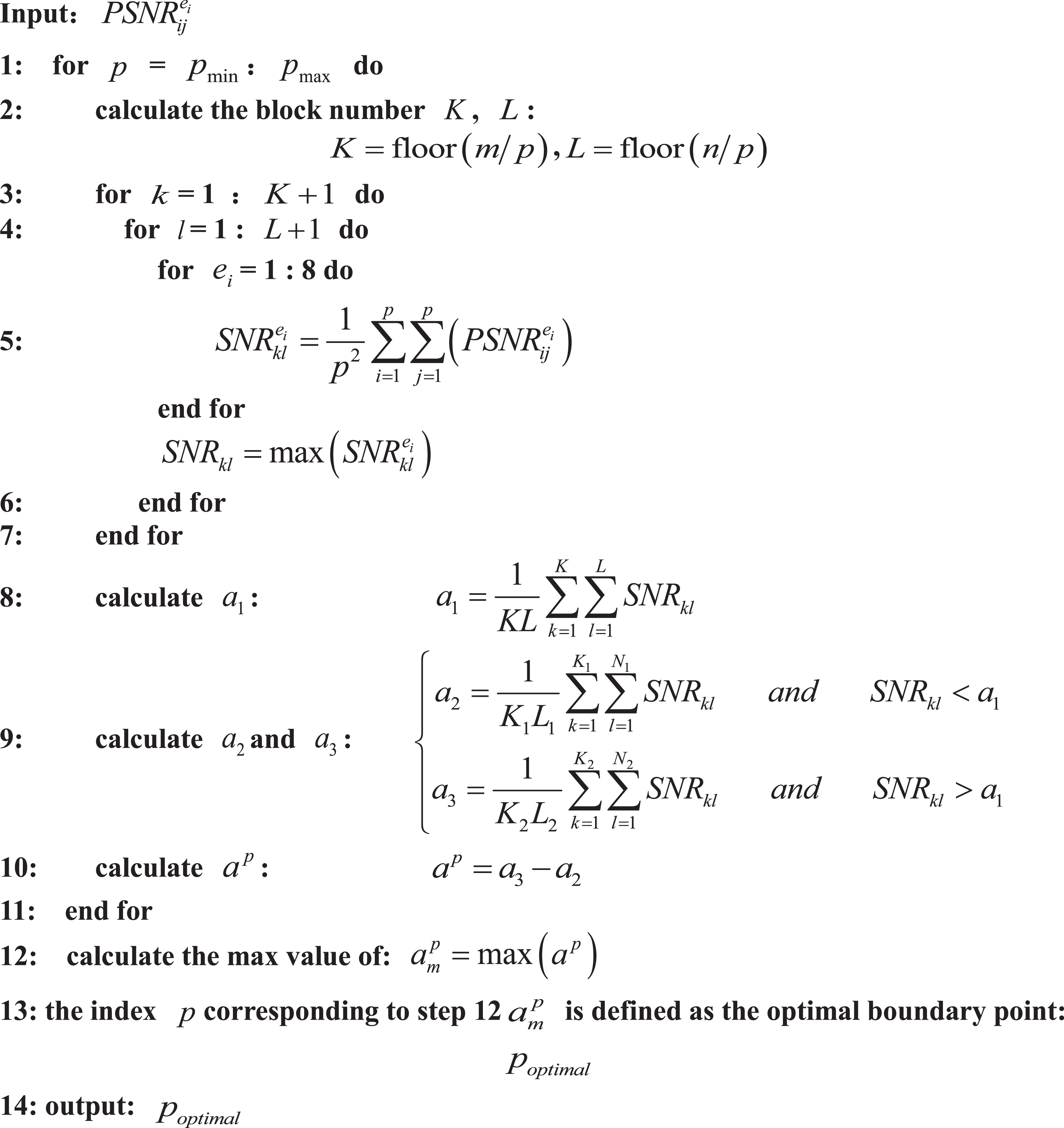
With changes in the mesh size, the suitable area and unsuitable area has been parted not different blocks or in the same block. The problem we care about is whether there is a mesh size that can divide the suitable area and the unsuitable area into different mesh as much as possible. Next, we will study the partition method. Our research object is the DEM as shown in Figure 6. The previous content has studied the method of terrain suitability quantification. On this basis, the following sections will introduce the partition method of the suitable area and the unsuitable area. First, we quantify the suitability of DEM according to the previous method. Then, we further discuss the solution of partition of the suitable area and the unsuitable area optimally. The suitability of DEM can be quantified as following steps:

1. Calculate the SNR value of node $(k, l)$ at eight directions, the results are shown in Figure 7(a) to (h).

{PSNR}_{i j}^{e_{i}} = \frac{1}{σ_{​}^{2}} {({\hat{h}}_{i j} (X_{​}^{t}) - {\hat{h}}_{i j} (X_{​}^{t} + d • e_{i}))}^{2}

2. The size of the mesh is defined by the number of nodes on the edge of mesh. The interval of the number of nodes on the edge of the mesh is $[p_{min}, p_{max}]$ , $p_{min}$ , and $p_{max}$ are determined by the strip width of multi-beam. It’s best to stay near the width of the multi-beam strip, we defined $p_{min} = 0.75 b$ and $p_{max} = 1.25 b$ . For each block $(k, l)$ , assuming that the mesh size is $p \times p$ , p represents the number of nodes on the mesh edge and according to equation (7), the information value of the eight direction of block $(k, l)$ is calculated.

I_{e_{i}}^{p} (k, l) = - \frac{1}{p^{2}} \sum_{i = 1}^{p} \sum_{j = 1}^{p} {PSNR}_{i j}^{e_{i}}

3. Obtain the quantitative expression of terrain suitability of the block $(k, l)$ according to equation (9)

{SNR}_{k l}^{​} = min (I_{e_{i}}^{p} (k, l))

Figure 6.

The DEM used in this article. DEM: digital elevation map.

Figure 7.

Discrete information content for eight directions of DEM. DEM: digital elevation map.

Assumed that when the block size is $p \times p$ , the partition number of the DEM is $K \times L$ . We can obtain the following suitability matrix ${SNR}_{}^{p}$

{SNR}_{​}^{p} = [\begin{matrix} {SNR}_{11}^{​} & {SNR}_{12}^{​} & ... & {SNR}_{1 L}^{​} \\ {SNR}_{21}^{​} & {SNR}_{22}^{​} & ... & {SNR}_{2 L}^{​} \\ ... & ... & {SNR}_{k l}^{​} & ... \\ {SNR}_{K 1}^{​} & {SNR}_{K 2}^{​} & ... & {SNR}_{K L}^{​} \end{matrix}]

${SNR}_{k l}^{}$ indicates the suitability of each subblock $(k, l)$ with the block size $p \times p$ .

Partition of suitable and unsuitable area optimally

Now we can quantify the suitability of each block. Our goal is to divide the suitable area and the unsuitable area into different terrain blocks as far as possible. According to the previous analysis, the larger the $S N R_{k l}^{}$ value is, the higher the block suitability is. It is assumed that the mean of suitability sequence $S N R_{k l}^{}, k = 1, 2... K, l = 1, 2... L$ is a ₁ under the subblock size is $p \times p$ , the average of high suitability sequence $S N R_{k l}^{}, k = 1, 2... K_{1}, l = 1, 2... L_{1}$ is a ₂, and the average of low suitability sequence ${SNR}_{k l}^{}, k = 1, 2... K_{2}, l = 1, 2... L_{2}$ is $a_{3}$ , and their definitions are shown in equation (14)

{\begin{cases} a_{1} = \frac{1}{K L} \sum_{k = 1}^{K} \sum_{l = 1}^{L} {SNR}_{k l} \\ a_{2} = \frac{1}{K_{1} L_{1}} \sum_{k = 1}^{K_{1}} \sum_{l = 1}^{N_{1}} {SNR}_{k l} \begin{matrix} ​ & and & ​ \end{matrix} {SNR}_{k l} < a_{1} \\ a_{3} = \frac{1}{K_{2} L_{2}} \sum_{k = 1}^{K_{2}} \sum_{l = 1}^{N_{2}} {SNR}_{k l} \begin{matrix} ​ & and & ​ \end{matrix} {SNR}_{k l} > a_{1} \end{cases}

In the equation, K and L represent the rows number and columns number of map blocks; a ₁ represents the average of SNR of map block under the blocks number of $K \times L$ ; a ₂ represents the average of SNR of map block which is smaller than a ₁; $K_{1} L_{1}$ represent the sum of map block in which the SNR is smaller than a ₁; a ₃ represents the average of SNR of map block in which SNR is larger than a ₁; $K_{2} L_{2}$ represent the sum of blocks in which the SNR is smaller than a ₂. As shown in Figure 8, the suitability closer to the left end point indicates that the block belongs to the high suitable block, and the suitability close to the right end point indicates that the block belongs to the unsuitable block. While the block in the middle part indicates that the suitable area and unsuitable area are not yet effectively separated. We hope that a ₂ and a ₃ can be as possible as close to the left and right end point. So, $a_{}^{p}$ is used as shown in equation (15) to show the distance between them. So, $a_{}^{p}$ is the evaluation coefficient of partition quality of DEM and taking a larger value is beneficial as shown in Figure 9.

a_{​}^{p} = a_{3} - a_{2}

Figure 8.

A good partition indicate that the average of suitability of all high suitability blocks and the average of suitability of all low suitability blocks close to right and left end point.

Figure 9.

Relationship curve between the number of block side nodes and the block evaluation index $a^{p}$ .

According to the above requirements, we establish the constraint conditions for an optimal block. Based on the above analysis, a mathematical description of optimal block is obtained. In the process of optimal partitioning, we must to determine the range of the block sizes. The value interval is based on the measurement range of multi-beam sonar, supposing that the maximum and minimum values of the number of block side nodes are ${dep}_{max}$ and ${dep}_{min}$ , respectively. The optimal p value calculation process is described as follows.

According to the above analysis, we can obtain the optimal block of the DEM. Next, we calculated and analyzed an actual submarine topography as shown in Figure 6. The size of DEM is $891 \times 922 m^{2}$ , and the grid size of DEM is $1 \times 1 m^{2}$ . According to the description of Algorithm 1, a relationship curve between the number of block side nodes and the block evaluation index $a^{p}$ can be obtained. As can be seen from Figure 8, the value of $a^{p}$ changes dramatically with increases in the number of the block side nodes, and the maximum value is obtained when the value increases to 87.

Algorithm 1.

Calculate the optimal block

As shown in Figure 10, the block results are obtained according to the 87 boundary nodes. Figure 10(a) shows the SNR of each subblock, while Figure 10(b) shows the DEM results.

Figure 10.

DEM and its gridding results. DEM: digital elevation map. (a) Gridding of adaptation map; (b) Optimal gridding result of DEM.

TRP comparison and analysis of suitability block

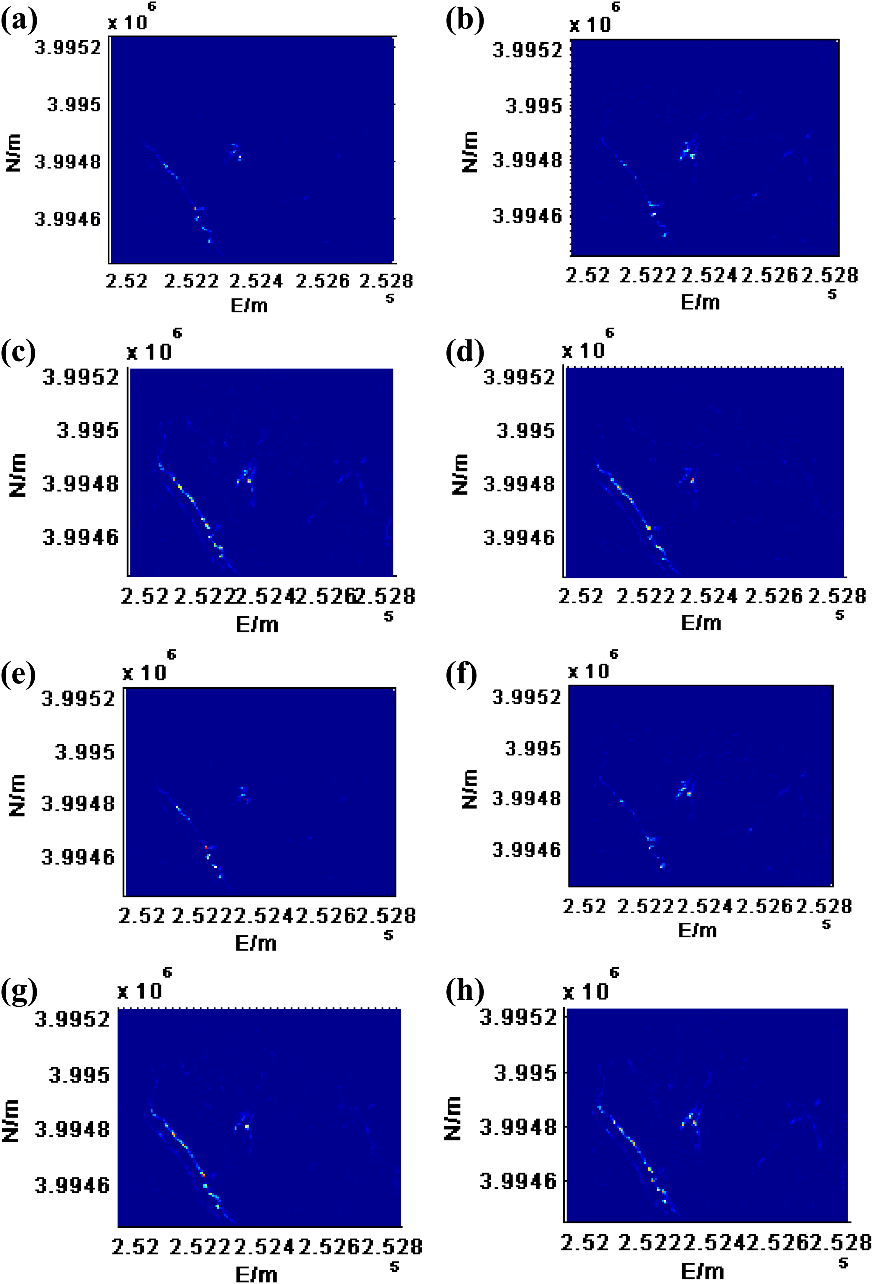
The validity of the suitability region segmentation is shown below. The DEM map will provide the priori information and the MTM will be used to simulate the real-time surveying terrain. We evaluate the effectiveness of the optimal partition algorithm by comparing the TRP accuracy in high suitability blocks and low suitability blocks. In the DEM (Figure 6) and the MTM (Figure 11), they have surveyed in the same sea area as shown in Figure 12. The DEM survey was taken in 2012 and the MTM measurement time was October 2016. Figure 13 shows the connection of measurement equipment while surveying MTM. The measurement device and their parameters are shown in Appendix Table 1A.

Figure 11.

The DEM map and the MTM map used in the simulation. DEM: digital elevation map; MTM: measurement terrain map.

Figure 12.

Location of DEM. DEM: digital elevation map.

Figure 13.

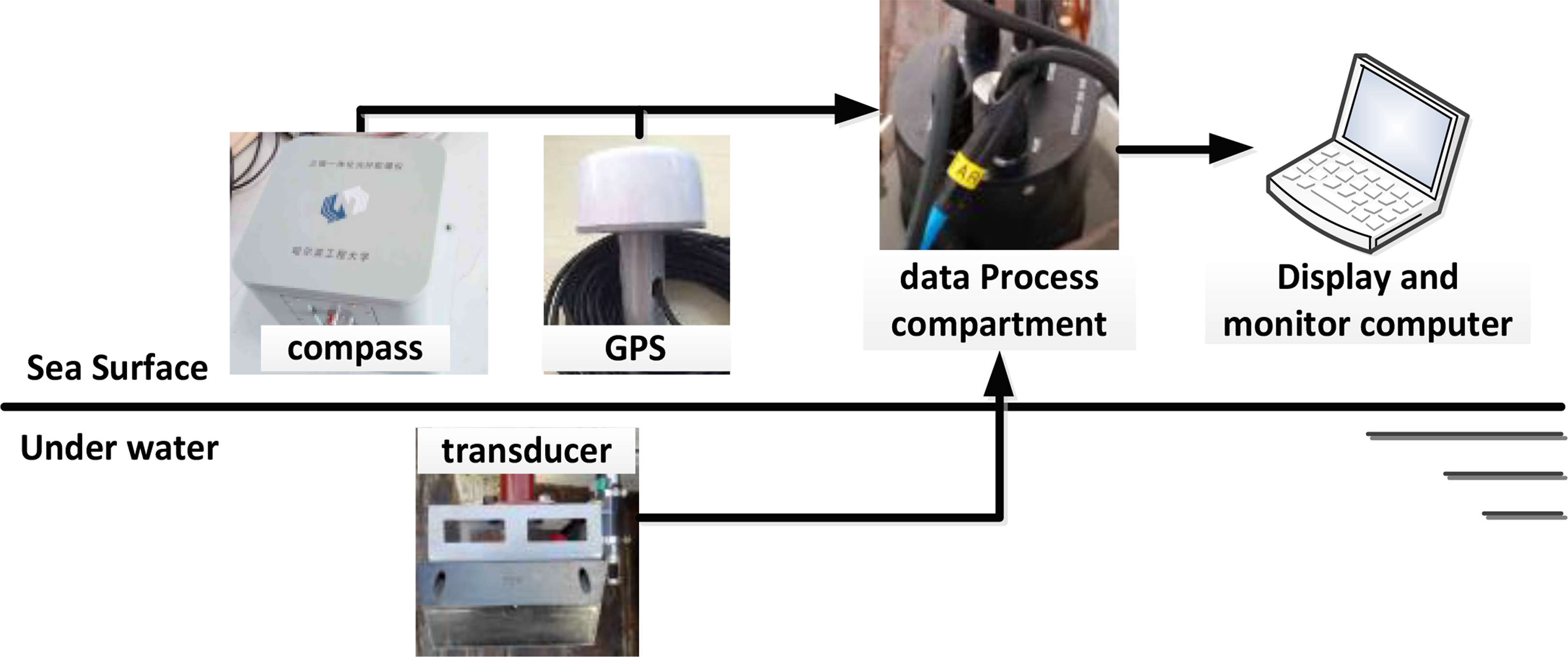
Topographic map surveying equipment and their connections.

Comparison of commonly quantitative parameters

We compare the quantitative method proposed in this article with the two commonly used terrain adaptation quantization methods (topographic entropy and topographic standard deviation).^10,18,19 The expressions of topographic entropy and topographic standard deviation are as follows:

1. Topographic entropy H

{\begin{cases} \bar{z} = \frac{1}{m n} \sum_{i = 1}^{m} \sum_{j = 1}^{n} (z_{i j}) \\ c_{i j} = \frac{| z_{i j} - \bar{z} |}{\bar{z}} \\ p_{i j} = \frac{c_{i j}}{\sum_{i = 1}^{m} \sum_{j = 1}^{n} (c_{i j})} \\ H = - p_{i j} \sum_{i = 1}^{m} \sum_{j = 1}^{n} log (p_{i j}) \end{cases}

In the equation, the number of nodes that measure the terrain is $m \times n$ and, $(i, j)$ is the index number that represents the measurement of a topographic node.

2. The standard deviation of terrain S

{\begin{cases} \bar{z} = \frac{1}{m n} \sum_{i = 1}^{m} \sum_{j = 1}^{n} (z_{i j}) \\ S = \frac{1}{m n - 1} \sum_{i = 1}^{m} \sum_{j = 1}^{n} {(z_{i j} - \bar{z})}^{2} \end{cases}

We use the MTM1 (Figure 3(a)) and MTM2 (Figure 3(b)) as a contrast experiment. From Figure 3(c) and (d) we can see that the gradient of MTM1 has a distinct directional distribution, but the direction of MTM2 is not obvious. The suitability of MTM1 and MTM2 are compared using the suitability parameters SNR, Terrain Entropy, and Terrain Standard Deviation, respectively. The test result shown in Figure 13, and the deviation average and standard deviation of TRP deviation shows that the suitability of MTM2 is better than that of MTM1. The SNR of MTM1 is smaller than MTM2, and it shows that the suitability of MTM2 is better than that of MTM1, but Terrain Entropy and Terrain Standard Deviation of MTM1 and MTM2 are almost the same. The major reason is that the Terrain Entropy and Terrain Standard Deviation can’t show the characteristics of anisotropy of terrain. As one of the most important features of terrain suitability is its directionality, and the most important feature of the suitability quantization parameter SNR used in this article is the ability to show the orientation of suitability.

Table 1.

Terms and abbreviations.

Autonomous underwater vehicle	AUV	Point mass filter	PMF
Terrain reference position	TRP	Particle filter	PF
Terrain reference navigation	TRN	Digital elevation map	DEM
Inertial navigation system	INS	Signal noise ratio	SNR
Real-time measurement terrain map	MTM	Global positioning system	GPS
Terrain information content	TIC

TRP accuracy of path in different suitability blocks

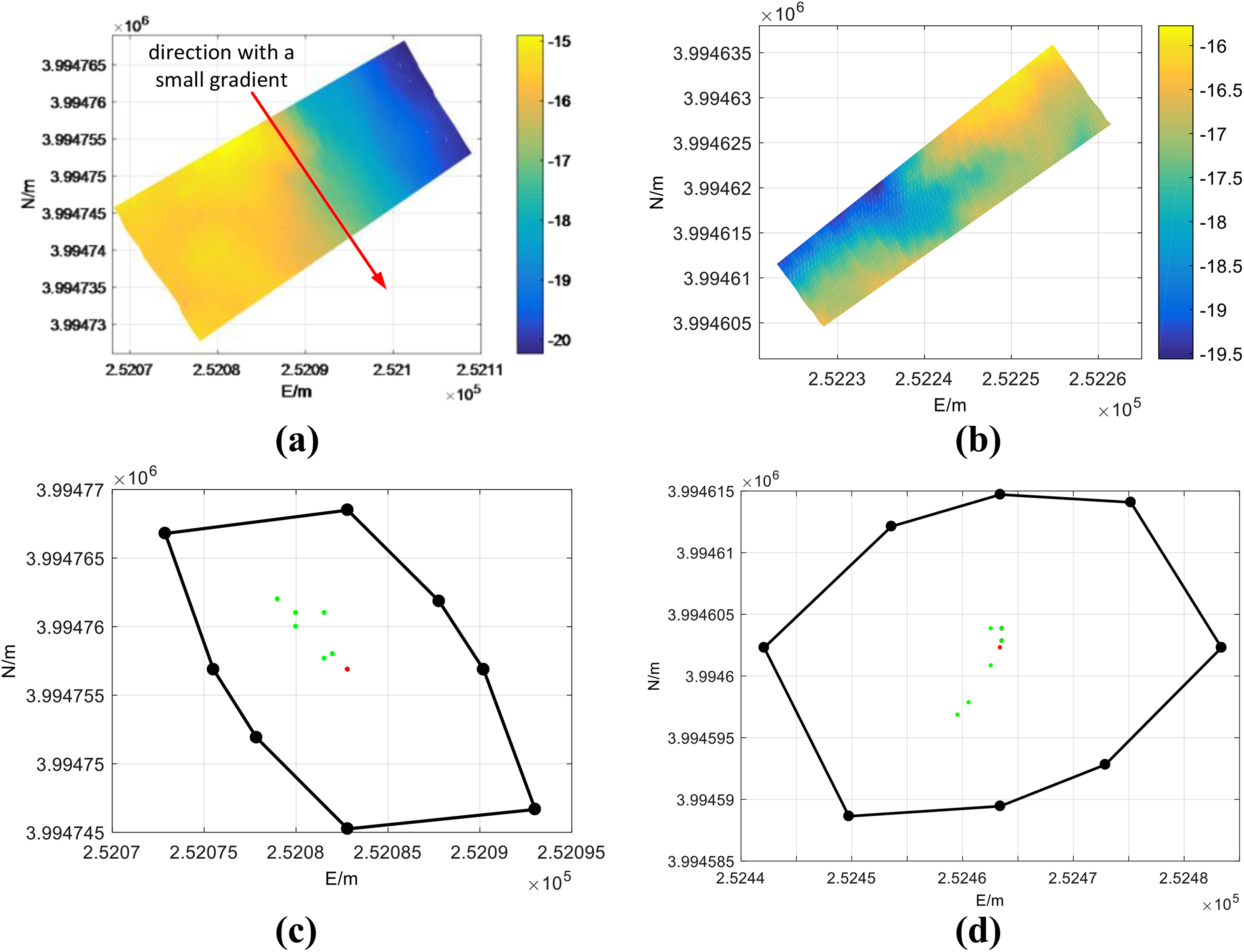
As shown in Figure 15(a), we choose suitable blocks and unsuitable blocks from the suitability map (Figure 15(a)). The unsuitable blocks and the suitable blocks are marked in white rectangle (marked A and B in Figure 15(a)) and red rectangle (marked C in Figure 15(a)), respectively. The suitability average of unsuitable blocks is 0.007, and the suitability average of suitable blocks is 0.019. The planning path (red line) and waypoints (green dots) in the suitable blocks and unsuitable blocks are shown in Figure 15(a). The simulated real-time measurement terrain is obtained by interpolation in the Figure 14 along the planning path as shown in Figure 15(a), and the simulated real-time measurement terrain are shown in Figure 15(b) and marked as a, b, c, respectively. To compare the position accuracy of high suitable blocks and unsuitable blocks under the condition of different measurement error. The design of comparative experiments is as follows:

The terrain blocks in red rectangles (marked as A and B) shown in Figure 15(a) are unsuitable terrain blocks. The terrain blocks in white rectangle (marked as C) shown in Figure 15(a) are suitable terrain blocks.

To simulate different measurement error conditions, the Gauss white noise added to the simulated measurement terrain map are $σ = 0.4$ and $σ = 0.9$ respectively.

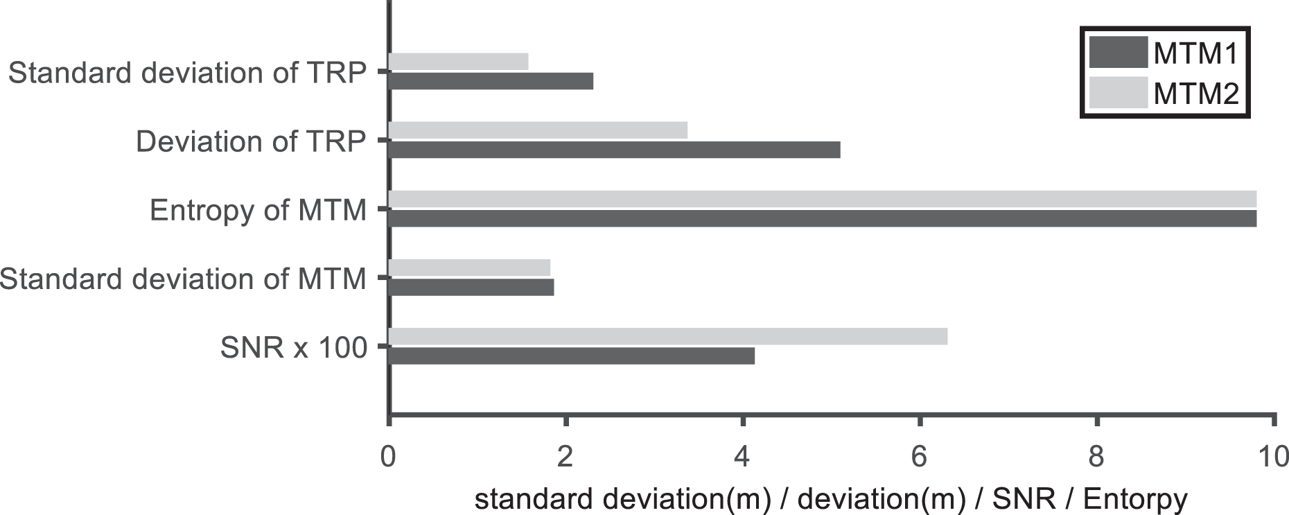
Repeat 10 times positioning simulation under the noise of $σ = 0.4$ and $σ = 0.9$ , respectively, using the average and standard deviation of TRP deviation as accuracy evaluation.

Figure 14.

Comparison of position accuracy and quantization parameters of MTM1and MTM2. TRP: terrain reference position; MTM: measurement terrain map; SNR: signal noise ratio.

Figure 15.

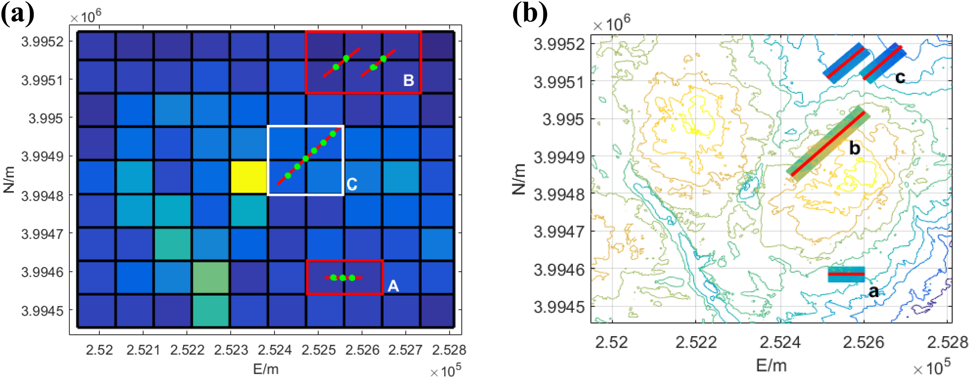
The data used in the simulation experiment. (a) The suitability map of DEM, high suitable blocks (C), low suitable blocks (A, B), and waypoint (•). (b) The counter map of DEM and planning measurement path (__), MTM. MTM: measurement terrain map; DEM: digital elevation map.

Finally, we get the statistical results of TRP positioning accuracy as shown in Figures 16 and 17.

Figure 16.

Statistical accuracy of positioning accuracy in suitable blocks (SNR = 0.019) and unsuitable blocks (SNR = 0.007), when the measurement error is 0.4. SNR: signal-to-noise ratio.

Figure 17.

Statistical accuracy of positioning accuracy in suitable blocks (SNR = 0.019) and unsuitable blocks (SNR = 0.007), when the measurement error is 0.9. SNR: signal-to-noise ratio.

From the results of Figures 16 and 17, we can see that when the suitability of the terrain block is SNR = 0.019 and the measurement error is 0.4, the average of TRP deviation is 3.69 m and the standard deviation of TRP deviation is 1.93 m. When the measurement error is 0.9, the average of the TRP deviation is 4.18 m and the standard deviation of TRP deviation is 1.96 m. The average of TRP deviation is increased by 13.3%, and the standard deviation of TRP deviation is increased by 1.6%. When the suitability of the topographic block is SNR = 0.007 and the measurement error is 0.4, the average of TRP deviation is 8.13 m and the standard deviation of TRP deviation is 5.62 m. When the measurement error is 0.9, the average of the TRP deviation average of the TRP is 9 m and the standard deviation of TRP deviation is 7.25 m. The average of TRP deviation is increased by 9.7%, and the standard deviation of TRP deviation is increased by 29%. The experiment shows that the TRP accuracy in suitable blocks will be better than that of unsuitable blocks. In addition, the standard deviation of TRP deviation in the suitable blocks will increase faster than that of the unsuitable blocks when the measurement error increased. That is to say, in the low suitable blocks, the TRP accuracy will be affected by the measurement error more easily.

Accuracy comparison between different suitability paths

The simulation process is shown in Figure 18. At first, the DEM is gridded as shown in Figure 10, and the high suitability area and the low suitability area are separated using the method proposed in the previous part. Then, we plan two paths (path A and path B), path A passes through the high suitability blocks and path B passes through the low suitability blocks. Next, we use the planning path (path A and path B) to interpolate in MTM (Figure 11), simulate the real-time measurement process of multi-beam, and get the simulated terrain along the path. Then, the simulated path (path A and path B), the simulated terrain, and DEM are put into the TRP system.

Figure 18.

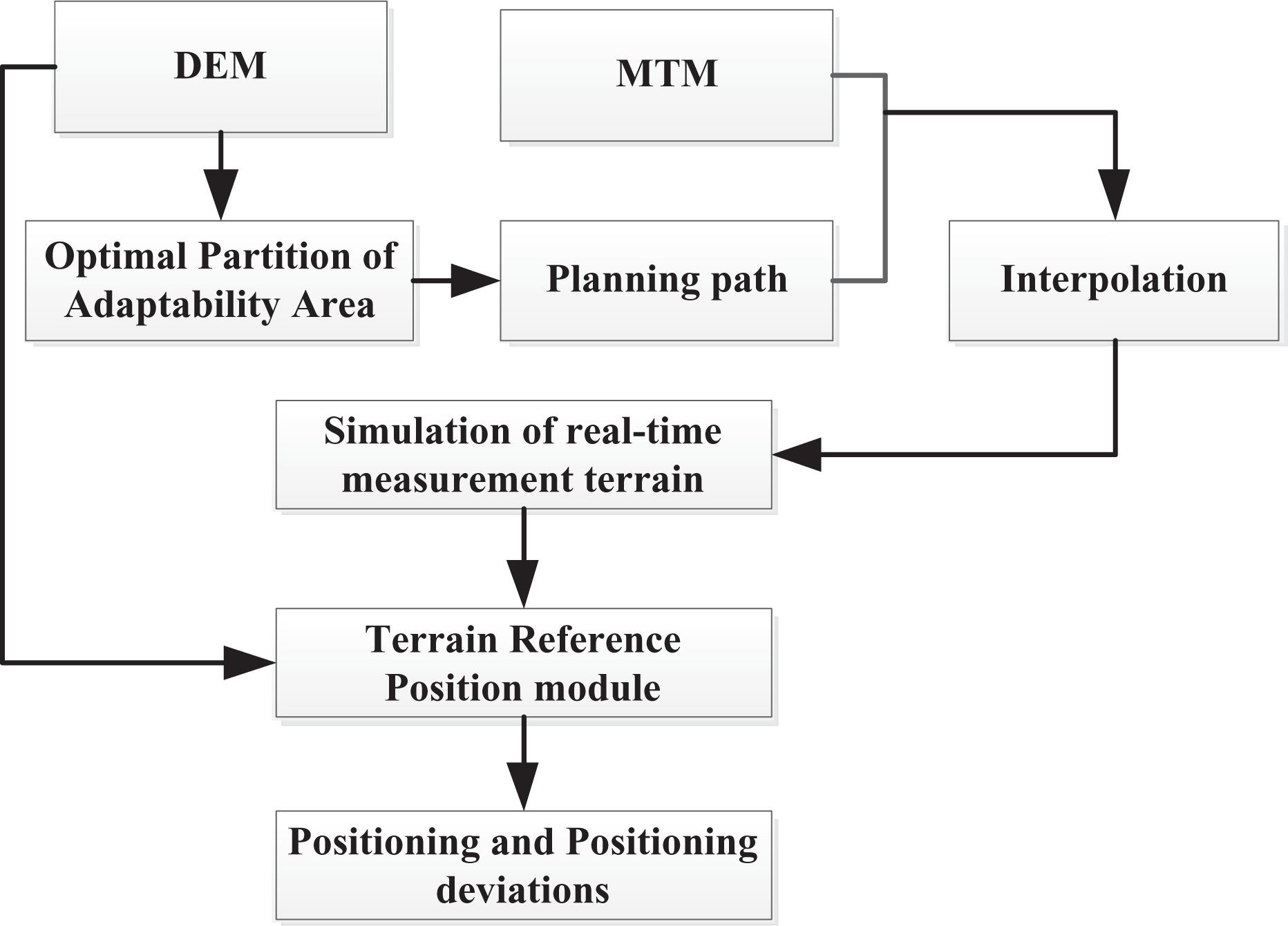
Flow chart of TRP simulation system. TRP: terrain reference positioning.

The planning path in the DEM is shown in Figure 19. Figure 19(a) and (b) show the location in the DEM and SNR map of path A, and the green dots are waypoints. As the same, Figure 19(c) and (d) shows path B. In addition, the block covered by path A will have bigger SNR values than those of path B.

Figure 19.

Two tested planning path and waypoints for path A and path B. (a) Path A and the waypoints in the DEM, (b) path A pass through high suitability blocks, (c) path B and the waypoints in the DEM, and (d) path B pass through high suitability blocks. DEM: digital elevation map.

Figure 20 shows the TRP result of path A through the high suitability block. Figure 20(a) shows the distribution of simulation of real-time measurement map and TRP points (•), while the SNR values of the covered block are shown in Figure 20(b). The SNR values are greater than 0.02. Figure 20(c) shows the TRP deviation at each waypoint. From the figure, we can see that the TRP deviation is limited below $6.5 m$ .

Figure 20.

TRP results for the route through the high SNR block. (a) Path A and the simulated real-time measurement terrain at waypoints, (b) the suitability value of the blocks that path A pass through, and (c) the position deviation of the waypoints in path A. TRP: terrain reference positioning; SNR: signal-to-noise ratio.

Figure 21 shows the TRP results for path B pass through the low suitability block. Figure 21(a) shows the distribution of MTM and TRP points (•), while the SNR values of the covered block are shown in Figure 21(b). The SNR values are below 0.02. Figure 21(c) shows the TRP deviation at each waypoint. From the figures, we can see that the TRP stability of path B is lower than path A (Figure 19). In blocks 5 and 6, the TRP deviation increases sharply.

Figure 21.

TRP results with the route through the high SNR block. (a) Path B and the simulated real-time measurement terrain at waypoints, (b) the suitability value of the blocks that path B pass through, (c) the position deviation of the waypoints in path B. TRP: terrain reference positioning.

Figure 22 shows a comparison of TRP results for the two routes. As we can see, the average and standard deviation for TRP deviation along path B (the low SNR path) is larger than that for path A (the high SNR path). Path A, through a terrain block with high SNR, and path B, through a terrain block with low SNR. From the TRP results, we can see that path A produces more accurate TRP positions, and the result is more stable.

Figure 22.

TRP position comparing path A and path B. TRP: terrain reference positioning.

Conclusions

The main contribution of this article is to propose the terrain suitability parameter SNR and global map gridding method based on partition of suitable area and unsuitable area optimally. The difference with the commonly used quantitative parameters is that SNR not only takes the measurement error of terrain, the change in rate of terrain gradient into account, but also takes the directional characteristics of adaptation into account. The simulation experiment shown that the influence of measurement error on TRP accuracy is higher than that in high suitability area, and higher positioning accuracy and stability can be obtained in the high suitability blocks. Notably, the optimal partition criterion in this article is that the maximum distance between the average of high suitability blocks and the suitability of the low suitability blocks. This optimal criterion is not the only one and there may be a better criterion. In addition, the next goal is to establish a more perfect underwater environment information map, including underwater threats, task location, priorities, and so on. In this way, AUV can plan an optimal path independently according to the task requirements and environmental threats, navigation errors, terrain suitability, and other factors.

Footnotes

Declaration of conflicting interests

The author(s) declared no potential conflicts of interest with respect to the research, authorship, and/or publication of this article.

Funding

The author(s) disclosed receipt of following financial support for the research, authorship, and/or publication of this article: This study is supported by the Central University Freedom Exploration Fund (Projects GK2010260235) and National Key Research and Development Plan (No. 2017YFC0305700).

ORCID iD

Li Ye

Cong Zheng

Appendix 1

Table 1A.

Major measure device parameters.

	Compass	Topography measurement device
Device name	Harbin engineering university self-developed fiber-optic gyro	Geo Swath Plus
Specifications	Temperature bias stability: 0.05° h⁻¹	Maximum water depth: 50 m
	Random walk: 0.0025° h⁻¹	Depth resolution: 1.5 mm
	Angular resolution: 0.2 arc s	Max Swath update rate: 30 s⁻¹

References

Chen

. A study on underwater terrain matching aided navigation technology of AUV. Doctoral Thesis, Harbin Engineering University, Harbin, 2013, pp. 19–20.

Nygren

. Terrain navigation for underwater vehicles. Doctoral Thesis, KTH Royal Institute of Technology, Sweden, 2005, pp. 30–35.

Murangira

Musso

Dahia

. Robust regularized particle filter for terrain navigation. In: Proceedings of the international conference on information fusion, July 2011, pp. 1–8. IEEE.

Teixeira

Pascoal

Maurya

. A novel particle filter formulation with application to terrain-aided navigation. In: IFAC workshop on navigation, guidance and control of underwater vehicles, 2012.

Donovan

. Development and testing of a real-time terrain navigation method for AUVs. In: OCEANS’11 MTS/IEEE KONA, Waikoloa, HI, USA, 19–22 September 2011. DOI: 10.23919/OCEANS.2011.6107009.

Claus

Bachmayer

. Terrain-aided navigation for an underwater glider. J Field Robot 2015; 32(7): 935–951.

Dektor

Rock

. Improving robustness of terrain-relative navigation for AUVs in regions with flat terrain. In: Autonomous underwater vehicles IEEE, Southampton, UK, 24–27 September 2012, pp. 1–7. DOI: 10.1109/AUV.2012.6380751.

Sutton

Bla Karlsson

Gustafsson

. Particle filter for underwater terrain navigation. In: 2003 IEEE workshop on statistical signal processing, 2003, pp. 526–529. IEEE.

Teixeira

Quintas

Maurya

. Robust particle filter formulations with application to terrain-aided navigation: Robust particle filters for terrain-aided navigation. Int J Adapt Control Signal Process Marine Syst 2016; 31(4): 608–651.

10.

Hagen

Ånonsen

Skaugen

. Robust surface vessel navigation using terrain navigation. In: Oceans IEEE, Bergen, Norway, 10–14 June 2013, pp. 1–7. DOI: 10.1109/OCEANS-Bergen.2013.6608055.

11.

Anonsen

Hallingstad

. Terrain aided underwater navigation using point mass and particle filters. In: Position, location, & navigation symposium, IEEE/ION IEEE, Coronado, California, USA, 25–27 April 2006, pp. 1027–1035. DOI: 10.1109/PLANS.2006.1650705.

12.

Yoo

Chan

. Improvement of terrain referenced navigation using a point mass filter with grid adaptation. Int J Control Autom Syst 2015; 13(5): 1173–1181. DOI: 10.1007/s12555-013-0410-4.

13.

Feng

. Study on the new method and environmental adaptability of the terrain matching. PhD thesis, National University of Defense Technology, Chang Sha, 2004, pp. 91–106.

14.

Dektor

Rock

. Robust suitable terrain-relative navigation. In: Oceans – St. John’s IEEE, St. John’s, NL, Canada, September 2014, pp. 1–10. DOI: 10.1109/OCEANS.2014.7003195.

15.

Teixeira

Quintas

Maurya

. Robust particle filter formulations with application to terrain-aided navigation. IFAC Proc 2017; 45(4): 132–139. DOI: 10.1002/acs.2692.

16.

Teixeira

Quintas

Maurya

. Robust particle filter formulations with application to terrain-aided navigation. IFAC Proc 2012; 45(5): 132–139. DOI: 10.3182/20120410-3-PT-4028.00023.

17.

Melo

Matos

. Survey on advances on terrain based navigation for autonomous underwater vehicles. Ocean Eng 2017; 139: 250–264.

18.

Krukowski

Rock

Waypoint planning for autonomous underwater vehicles with terrain relative navigation. In: OCEANS 2016 MTS/IEEE Monterey, Monterey, CA, USA, 19–23 September 2016. DOI: 10.1109/OCEANS.2016.7761180.

19.

Häusler

Saccon

Pascoal

. Cooperative AUV motion planning using terrain information. In: Oceans IEEE, 2013, pp. 1–10. DOI: 10.1109/OCEANS-Bergen.2013.6608137.

20.

Franca

Saltón

Castro

RDS

. Trajectory generation for bathymetry based AUV navigation and localization. IFAC Papers Online 2015; 48(16): 95–100. DOI: 10.1016/j.ifacol.2015.10.264.

21.

Chen

. Autonomous underwater vehicle optimal path planning method for seabed terrain matching navigation. Ocean Eng 2017; 133(10): 107–115. DOI: 10.1016/j.oceaneng.2017.01.026.

22.

Chaari

Koubaa

Bennaceur

. Design and performance analysis of global path planning techniques for autonomous mobile robots in grid environments. Int J Adv Robot Syst 2017; 14(2). DOI: 10.1177/1729881416663663.

Underwater digital elevation map gridding method based on optimal partition of suitable matching area

Abstract

Keywords

Introduction

Suitability and TRP Accuracy

Influencing factors on TRP accuracy

Accuracy evaluation of TRP

Terrain suitability quantification

Optimal partition of terrain suitable area

Suitability quantization of DEM under arbitrary gridding

Partition of suitable and unsuitable area optimally

TRP comparison and analysis of suitability block

Comparison of commonly quantitative parameters

TRP accuracy of path in different suitability blocks

Accuracy comparison between different suitability paths

Conclusions

Footnotes

Declaration of conflicting interests

Funding

ORCID iD

Appendix 1

References