Underwater terrain-aided navigation method based on improved Gaussian sum particle filtering

Abstract

To solve the nonlinear Bayesian estimation problem in underwater terrain-aided navigation, a terrain-aided navigation method based on improved Gaussian sum particle filter is proposed. This method approximates the Bayesian function using multiple Gaussian components, and the components can be obtained by radial basis function neural network. This method has no resampling process, the particle depletion of particle filtering is eliminated in principle. The simulation shows that the proposed method has good matching performance, which is suitable for autonomous underwater vehicle navigation.

Introduction

Underwater terrain-aided navigation (UTAN) has the advantages of low cost, long-term, concealed, all-weather, and so on, which is a hotspot in the field of underwater autonomous navigation. ¹ A number of research institutions and organizations working on related technology research have developed some corresponding hardware and software systems and conducted sea trials. ^{2 –4}

Using terrain height change information, the carrier position can be estimated by UTAN algorithm. Because of the strong nonlinear characteristics of underwater terrain, the UTAN is a nonlinear estimation problem. Therefore, the posterior probability density function cannot be obtained directly, which can only use the approximate models. Generally, the approximate models can be divided into two categories. One is to transform the nonlinear model into a linear model using Taylor expansion, then use Kalman filtering to process the linear model, which is called for extended Kalman filter (EKF). Due to the strong nonlinearity, the real terrain is not necessarily approximated by first-order Taylor expansion, EKF has the risk of non-convergence. ⁵ The other solution is to retain the nonlinear model, the posterior probability density is approximately expressed. Bergman et al. ⁶ first proposed the terrain-aided navigation (TAN) model for aircraft under the Bayesian framework and pointed out the problem substance is the nonlinear Bayesian posterior probability estimation. Then the particle filter (PF) were introduced to solve nonlinear Bayesian estimation of TAN, ⁷ which achieved very good results. Since then, PF has become a research hotspot of TAN algorithm.

The main defect of PF is the particle depletion caused by resampling, which will cause the sharp decline of PF performance. Aiming at this defect, many improved PF methods for TAN have been proposed in recent years. ^{8 –10} These methods improve and optimize the resampling process to increase particle diversity. Essentially, these methods can only postpone the particle depletion, instead of completely eliminated. Because the underwater terrain features are less than terrestrial terrain, the influence of particle depletion is more serious. Kotecha and Djuric ¹¹ proposes a Gaussian Particle Filtering (GPF), which use the Gaussian distribution function as the importance density function of PF, and there is no resampling process. Therefore, the particle depletion is eliminated in principle, and the calculation amount is also reduced without resampling.

In this article, the GPF will be introduced into UTAN and combined with Radial Basis Function Neural Network (RBFNN) ^12–13 and multiple Gaussian components, an improved RBFNN-based Gaussian Sum Particle Filtering (RBFNN-GSPF) method for UTAN is proposed. Simulation results show that the proposed method can improve terrain positioning accuracy effectively has strong robustness to terrain features, which is suitable for autonomous underwater vehicle (AUV) navigation.

System model of UTAN

The UTAN system is usually combined with Inertial Navigation System (INS). INS is used to provide coarse location information, then the matching operation of UTAN is executed nearby the coarse location, and the precise position can be obtained. There are two types of combination of UTAN and INS: tightly coupled and loosely coupled. Because the loosely coupled does not consider the sensor error, the system structure is simple and the robustness is better. Therefore, this article uses the loosely coupled mode for UTAN/INS combination model. The vertical coordinates of AUV can be measured by acoustic altimeter and water pressure sensor in real time, which have no cumulative error, so the vertical position need not to be considered in terrain matching. Therefore, the system model is as follows

$\{\begin{array}{l}{\mathit{x}}_{t+1}={\mathit{x}}_t+{\mathit{u}}_t+{\mathit{v}}_t\\ {\mathit{y}}_t=\mathit{h}\left({\mathit{x}}_t\right)+{\mathit{e}}_t\end{array}$

1

where, ${\mathit{x}}_t$ is the position of INS at time t, ${\mathit{u}}_t$ is the position change between adjacent positioning times, ${\mathit{v}}_t$ is the error of horizontal position, ${\mathit{y}}_t$ is the real-time sounding data at time t, $\mathit{h}(•)$ is the local Digital Terrain Map (DTM) data at ${\mathit{x}}_t$ , and ${\mathit{e}}_t$ is the sounding error. All errors are defined as Gaussian white noise.

UTAN algorithm

Gaussian particle filtering

Based on the Gaussian probability density functions, the system status can be approximated. Based on the Bayesian filtering model for UTAN proposed by Chen et al., ¹⁴ the probability density distribution can be approximated by Gaussian function $p(•)$ , and the GPF can be expressed as follows:

Measurement update

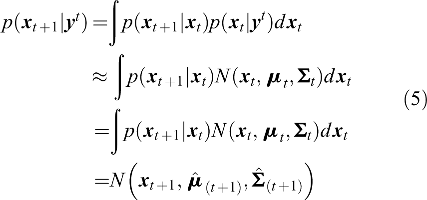
Assume that at time t, the predicted distribution of the system is as equation (2)

$p\left({\mathit{x}}_t|{\mathit{y}}^{t-1}\right)\text{=}N\left({\mathit{x}}_t,{\widehat{\mu }}_t,{\widehat{\Sigma }}_t\right)$

2

where, ${\widehat{\mathit{\mu }}}_t,{\widehat{\mathit{\Sigma }}}_t$ can be got by prior information. After getting the real-time sounding data at time t, the posterior probability density function can be obtained from equation (3)

$\begin{array}{l}p\left({\mathit{x}}_t|{\mathit{y}}^t\right)=\frac{p\left({\mathit{y}}_t|{\mathit{x}}_t\right)p\left({\mathit{x}}_t|{\mathit{y}}^{t-1}\right)}{p\left({\mathit{y}}_t|{\mathit{y}}^{t-1}\right)}\\ \text{ =}\frac{p\left({\mathit{y}}_t|{\mathit{x}}_t\right)N\left({\mathit{x}}_t,{\widehat{\mathit{\mu }}}_{ti},{\widehat{\mathit{\Sigma }}}_{ti}\right)}{p\left({\mathit{y}}_t|{\mathit{y}}^{t-1}\right)}\\ \propto p\left({\mathit{y}}_t|{\mathit{x}}_t\right)N\left({\mathit{x}}_t,{\widehat{\mathit{\mu }}}_{ti},{\widehat{\mathit{\Sigma }}}_{ti}\right)\end{array}$

3

According to Zhan et al., ¹⁵ the posterior distribution $p\left({\mathit{x}}_t|{\mathit{y}}^t\right)$ can be approximated by Gaussian distribution $N\left({\mathit{x}}_t,{\mathit{\mu }}_t,{\mathit{\Sigma }}_t\right)$ , and the ${\mathit{\mu }}_t,{\mathit{\Sigma }}_t$ can be obtained by the following equation set.

$\{\begin{array}{l}{\mathit{\mu }}_t={\widehat{\mathit{\mu }}}_t+{\mathit{K}}_t\left[{\mathit{y}}_t-{\mathit{h}}_t\left({\mathit{x}}_t\right)\right]\\ {\mathit{\Sigma }}_t={\widehat{\mathit{\Sigma }}}_t-{\mathit{K}}_t{\mathit{H}}_t{\widehat{\mathit{\Sigma }}}_t\\ {\mathit{K}}_t={\widehat{\mathit{\Sigma }}}_t{\mathit{H}}_t{\left({\mathit{H}}_t^T{\widehat{\mathit{\Sigma }}}_t{\mathit{H}}_t+{\sigma }_{\mathit{e}}^{2}I\right)}^{-1}\\ {\mathit{H}}_t\text{=}{\partial {\mathit{h}}_t\left(\mathit{x}\right)/\partial \mathit{x}|}_{\mathit{x}\text{=}{\widehat{\mathit{\mu }}}_t}\end{array}$

4

Time update

Since $p\left({\mathit{x}}_t|{\mathit{y}}^t\right)$ can be approximated by Gaussian distribution, thus, supposing further that $p\left({\mathit{x}}_{t+1}|{\mathit{y}}^t\right)$ is also a Gaussian distribution, that is

$\begin{array}{l}p\left({\mathit{x}}_{t\text{+}1}|{\mathit{y}}^t\right)\text{=}{\displaystyle \int p\left({\mathit{x}}_{t\text{+}1}|{\mathit{x}}_t\right)p\left({\mathit{x}}_t|{\mathit{y}}^t\right)d{\mathit{x}}_t}\\ \approx {\displaystyle \int p\left({\mathit{x}}_{t\text{+}1}|{\mathit{x}}_t\right)N\left({\mathit{x}}_t,{\mathit{\mu }}_t,{\mathit{\Sigma }}_t\right)d{\mathit{x}}_t}\\ \text{ =}{\displaystyle \int p\left({\mathit{x}}_{t\text{+}1}|{\mathit{x}}_t\right)}N\left({\mathit{x}}_t,{\mathit{\mu }}_t,{\mathit{\Sigma }}_t\right)d{\mathit{x}}_t\\ \text{ =}N\left({\mathit{x}}_{t\text{+}1},{\widehat{\mathit{\mu }}}_{\left(t\text{+}1\right)},{\widehat{\mathit{\Sigma }}}_{\left(t\text{+}1\right)}\right)\end{array}$

5

where, ${\widehat{\mathit{\mu }}}_{\left(t\text{+}1\right)}\text{=}\hspace{0.17em}{\mathit{\mu }}_t$ , ${\widehat{\mathit{\Sigma }}}_{\left(t\text{+}1\right)}\text{=}\hspace{0.17em}{\mathit{\Sigma }}_t\text{+}{\sigma }_{\mathit{v}}^{2}I$ . The state estimation and variance estimation of UTAN based on GPF can be calculated by following equations

${\widehat{\mathit{x}}}_t\hspace{0.17em}\text{=}\hspace{0.17em}{\mathit{\mu }}_t$

6

${\widehat{\mathit{\Sigma }}}_t\text{=}{\mathit{\Sigma }}_t\text{+}\left({\widehat{\mathit{x}}}_t-{\mathit{\mu }}_t\right){\left({\widehat{\mathit{x}}}_t-{\mathit{\mu }}_t\right)}^{\text{T}}$

7

In a strongly nonlinear system, Bayesian filtering model cannot be approximated well by single Gaussian distribution, which will cause the large filtering error. Lin et al. ¹⁶ proposes a GSPF method and a better approximation has been achieved. However, the method is computationally intensive, which is not suitable for high real-time systems. In this article, a GSPF based on RBFNN is proposed, which use RBFNN to calculate the weights of Gaussian components.

GSPF based on RBFNN

Generally, a RBFNN model consist of three layers: input layer, hidden layer, and output layer. The mapping from input layer to hidden layer is nonlinear, and the mapping from hidden layer to output layer is linear. Thus, the mapping from inputs to outputs are nonlinear, and the outputs are linear for tunable parameters. A typical structure of RBFNN is as Figure 1.

Figure 1.

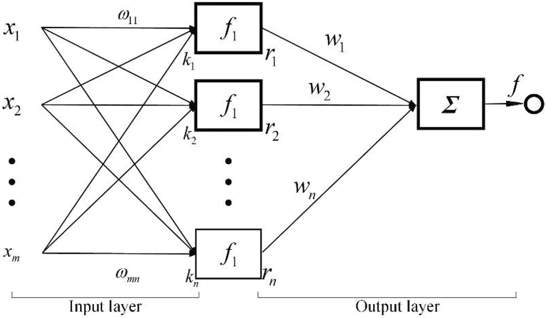
Typical structure of RBFNN. RBFNN: radial basis function neural network.

The structure of RBFNN is based on the function approximation theory. The learning process is searching the optimal matching surface in multidimensional space through the training data. The basic function of matching surface is formed by the activation functions of hidden layer. Based on the mixture of multiple Gaussian probability density functions, the system status can be approximated as follows

$p\left({\mathit{x}}_t|{\mathit{y}}^{t-1}\right)\text{=}{\displaystyle \sum _{i\text{=}1}^G{\alpha }_{ti}N\left({\mathit{x}}_t,{\widehat{\mathit{\mu }}}_{ti},{\widehat{\mathit{\Sigma }}}_{ti}\right)}$

8

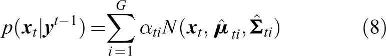
where G is the number of Gaussian components, ${\widehat{\omega }}_{ti}$ is the weight of the ith Gaussian component at time t. In this article, the Gaussian functions are used for radial basis functions. The input of RBFNN is as shown in equation (9)

$k_i=\sqrt{{\displaystyle \sum _{j=1}^m{\left({\omega }_{ji}-{\mathit{x}}_j\right)}^2}}\times \sqrt{\left(\text{lg}2\right)}/{\theta }_i$

9

where, ${\theta }_i$ is the adjustment parameter, which is equivalence to ${\widehat{\mathit{\Sigma }}}_i$ . The value of ${\theta }_i$ can be obtained by the required accuracy, generally, ${\theta }_i\hspace{0.17em}\approx \hspace{0.17em}0.5$ . Let the transfer function is $r\left(n\right)=\text{exp}\left(-n^2\right)$ . The output of RBFNN is as equation (10).

$f={\displaystyle \sum _{i=1}^n{r}_i\times w_i}$

10

Comparing with equations (8), (9), and (10), the following results will be acquired

${\alpha }_{ti}=w_i,\hspace{0.17em}{\widehat{\mathit{\mu }}}_{ti}={\displaystyle \sum _{j=1}^n{\omega }_{ji}},\hspace{0.17em}{\widehat{\mathit{\Sigma }}}_{ti}={\theta }_i^2/\text{lg}2$

11

RBFNN-GSPF method for UTAN

The process of RBFNN-GSPF method for UTAN is as follows:

1. Extract the samples from the system function and train network,

2. At time t, get the real-time sounding data ${\mathit{y}}_t$ and reference depth data $\mathit{h}\left({\mathit{x}}_t\right)$ .

3. Calculate the network parameters and get the initial weights, means, and covariances.

4. Measurement update:

• (a) The importance weight of particle is

  ${\lambda }_{tj}^i=p\left({\mathit{y}}_t|{\mathit{x}}_{tj}^i\right)N\left({\mathit{x}}_t\text{=}{\mathit{x}}_{tj}^i\text{, }{\widehat{\mathit{\mu }}}_{tj}\text{, }{\widehat{\mathit{\Sigma }}}_{tj}\right)/q\left({\mathit{x}}_{tj}^i|{\mathit{Y}}^k\right)$

  12

• (b) Calculate the mean and covariance of each Gaussian component.

• (c) Calculate the weights of each Gaussian component.

• (d) Weight normalization

  ${\alpha }_{tj}={\alpha }_{tj}/{\displaystyle \sum _{j=1}^G{\alpha }_{tj}}$

  13

5. Output state and variance estimates of matching result.

State estimate

${\widehat{\mathit{x}}}_t\text{=}{\displaystyle \sum _{j\text{=}1}^G{\alpha }_{tj}{\mathit{\mu }}_{tj}}$

14

Variance estimate

${\widehat{\mathit{\Sigma }}}_t\text{=}{\displaystyle \sum _{i\text{=}1}^G{\alpha }_{tj}\left[{\mathit{\Sigma }}_{tj}\text{+}\left({\widehat{\mathit{x}}}_t-{\mathit{\mu }}_{tj}\right){\left({\widehat{\mathit{x}}}_t-{\mathit{\mu }}_{tj}\right)}^{\text{T}}\right]}$

15

6. Time update

• (a) For Gaussian component j, select importance density function $q(•)={\alpha }_{tj}N\left({\mathit{x}}_t,{\widehat{\mathit{\mu }}}_t,{\widehat{\mathit{\Sigma }}}_{tj}\right)$ , then extract sample set $\left\{{\mathit{x}}_{tj}^i\right\}$ .

• (b) Based on the state transition distribution $p\left({\mathit{x}}_{\left(t+1\right)j}|{\mathit{x}}_{tj}={\mathit{x}}_{tj}^i\right)$ , the particles at time t + 1 are $\left\{{\mathit{x}}_{\left(t+1\right)j}^i\right\}$ .

• (c) Update weights ${\alpha }_{\left(t+1\right)j}={\alpha }_{tj}$ .

• (d) For Gaussian component j, update the forecast mean and forecast variance.

${\widehat{\mathit{\mu }}}_{\left(t+1\right)j}=\frac{1}{N}{\displaystyle \sum _{i=1}^N{\alpha }_{\left(t+1\right)j}{\mathit{x}}_{\left(t+1\right)j}^i}$

16

${\widehat{\mathit{\Sigma }}}_{\left(t+1\right)i}=\frac{1}{N}{\displaystyle \sum _{i=1}^N\left({\mathit{x}}_{\left(t+1\right)j}^i-{\widehat{\mathit{\mu }}}_{\left(t+1\right)j}\right){\left({\mathit{x}}_{\left(t+1\right)j}^i-{\widehat{\mathit{\mu }}}_{\left(t+1\right)j}\right)}^{\text{T}}}$

17

7. Based on equation (1), the position parameter ${\mathit{x}}_{t+1}^{}$ can be projected.

8. t = t + 1, go to step 2.

Simulation tests

The simulation tests are executed in an underwater semi-physical simulation system. The structure of the simulation system is shown in Figure 2.

Figure 2.

Semi-physical simulation system.

As shown in Figure 2, the simulation system includes three main parts: monitoring computer, environment simulation computer, and PC104 embedded computer. The PC104 is a real master computer of AUV, which is used for running the AUV control system. In semi-physical simulation tests, the sensor information is the data packet sent by environment simulation computer, and the actuator information is also sent to the environment simulation computer through Ethernet. The monitoring computer is used for displaying the “AUV” status information, and the monitoring interface is realized by Vega, and the intersecting rays of Vega ¹⁷ is used to simulate multi-beam sounding system (Figure 3).

Figure 3.

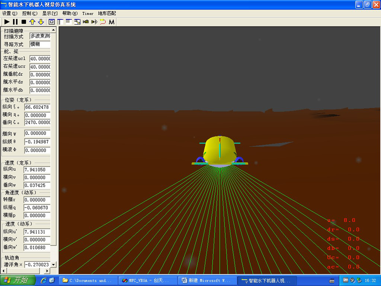
Monitoring interface.

The data source of DTM is real multi-beam sounding data measured in a sea trial. After filtering and gridding processing, a DTM can be obtained (Figure 4).

Figure 4.

DTM and navigation path. DTM: digital terrain map.

In Figure 4, the black line is the “AUV” navigation path in simulation tests. Based on different number of Gaussian components, number of particles, filtering cycle, and initial positioning error, the simulation tests are executed. The simulation parameters are shown in Table 1.

Table 1.

Simulation parameters.

Parameter name	Value
Error characteristic of INS	$N\left(0,{\left(0.05t\right)}^2\right)$ , t is the navigation time
Noise of “multi-beam measured”	$N\left(0,\hspace{0.17em}0.5\right)$
Other environmental noise	$N\left(0,\hspace{0.17em}0.5\right)$
“AUV” speed	4 kn
Data acquisition cycle	0.5 s

AUV: autonomous underwater vehicle; INS: inertial navigation system.

Simulation 1: Initial positioning error is 45 m, filtering cycle is 2 s, the number of particles is 2000, choose different number of Gaussian components, the simulation results are as Figure 5.

Figure 5.

Simulation results with different number of Gaussian components.

As a comparison, the simulation based on Improved Particle Filtering (IPF) method ¹⁸ is executed. As shown in Figure 5, the navigation accuracy and stability of proposed method is higher than IPF, thus, RBFNN-GSPF method has good matching performance. Also shown in Figure 5, with the number of Gaussian components increasing, the navigation accuracy of proposed method has not increased significantly. The average navigation accuracy with five Gaussian components is 3.24 m, and the average navigation accuracy with 20 Gaussian components is 3.02 m, the increased accuracy is very little. However, when the number of particles is the same, the amount of calculation is proportional to the number of Gaussian components. Therefore, five Gaussian components are the suitable choice.

Simulation 2: Initial positioning error is 50 m, the number of Gaussian components is 5, filtering cycle is 2 s, choose different number of particles, the simulation results are as Figure 6.

Figure 6.

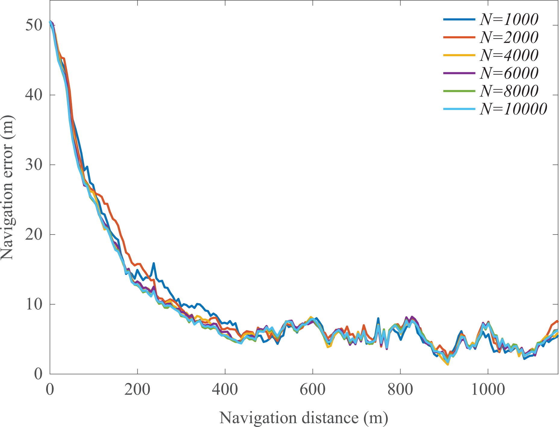
Simulation results with different number of particles.

As shown in Figure 6, the navigation results are similar with different number of particles. With the number of particles increasing, the convergence speed and steady-state of error interval are not improved significantly. Considering that calculation amount is proportional to the number of particles, thus 1000 particles are suitable.

Simulation 3: Initial positioning error is 50 m, the number of Gaussian components is 5, the number of particles is 1000, choose different filtering cycles, the simulation results are as in Figure 7.

Figure 7.

Simulation results with different filtering cycle.

As shown in Figure 7, the convergence time is inversely proportional to the filtering cycle. When the filtering cycle is 1 s, filtering can converge after about 100 m. On the contrary, when the filtering cycle is 32 s, filtering cannot converge until navigation end. However, the filtering cycle is 1 s, the steady-state of error interval is not good, this is because the data acquisition cycle is 0.5 s, such that the data amount for filtering is insufficient in a filtering cycle. Therefore, the filtering cycle should be considered comprehensively. Based on the simulation conditions used in this article, 2 s is a suitable filtering cycle.

Simulation 4: The number of Gaussian components is 5, the number of particles is 1000, filtering cycle is 2 s, choose different initial positioning error, the simulation results are as in Figure 7.

As shown in Figure 8, the convergence time is inversely proportional to the initial positioning error. The filtering can converge quickly with small initial positioning error, with the initial positioning error increasing, the time consumption of filtering convergence has also increased dramatically.

Figure 8.

Simulation results with different initial positioning error.

As can be seen from the above simulations, the filtering cycle and initial positioning error have a major impact on UTAN performance. The short filtering cycle and small initial positioning error can bring the fast convergence speed and relatively high navigation accuracy. This is because, the measurement update and the time update are corresponded, small initial positioning error makes the particle distribution close to the real range when updating, and the short filtering cycle can make the weight distribution of particles close to the real situation. GSPF uses multiple parallel Gaussian functions to approximate Bayesian estimation, so the filtering cycle and initial positioning error also affect the performance of PF-based terrain matching method.

Conclusions

An improved GSPF method for UTAN is proposed in this article. The Gaussian mixture components are gotten by RBFNN. The following conclusions can be reached:

The proposed UTAN method can correct the cumulative errors of INS.

Compared to PFs based on resampling technique, RBFNN-GSPF need not resample, which can bring the lower calculated amount.

With the number of Gaussian components increasing, the navigation accuracy is also slightly improved, however, the improvement is not obvious. Generally, 5–10 Gaussian components are suitable.

The performance of proposed method is sensitive to initial positioning error. Thus, it is valuable how to achieve the fast convergence with large initial error.