Active control of hydropneumatic suspension parameters of wheel loaders based on road condition identification

Abstract

Wheel loader is off-road vehicle and works on uneven terrain, unexpected banks or steep slopes. In order to improve the ride and stability of the vehicle, this study mainly focuses on how to adjust the parameters of hydropneumatic suspension through the identification of road conditions. Firstly, the multibody model of a wheel loader with hydropneumatic suspension is developed by RecurDyn in a co-simulation with MATLAB/Simulink. Secondly, a method of road level recognition based on learning vector quantization neural network is proposed to accurately identify the level of roads on which the wheel loader travels. Then, the hydropneumatic suspension parameters are optimized by using the particle swarm algorithm. A fuzzy controller is established based on the optimized parameters of the hydropneumatic suspension to realize the active adjustment of the suspension parameters under different road levels and driving speeds. Finally, a virtual prototyping model is used to analyse the influence of the active adjustment of suspension parameters on the vertical vibration under different driving conditions. Results show that the fuzzy controller can reasonably adjust the parameters of hydropneumatic suspension according to the identified road condition and effectively reduce the vertical vibration of the wheel loader.

Introduction

Wheel loaders are mainly used for removing topsoil, loading fragmented rock and ore from production bench and cleaning operation sites. These activities are tedious, and the weather conditions, which depend on geographical locations, are often harsh. ¹ In waste processing fields, wheel loaders are used for moving solid waste to landfill sites, and transporting soil to cover the waste. The trash material may contain radioactive substances, or have excitant odours. All these applications ask for the wheel loaders being automatically controlled. This will effectively improve operation safety, reduce the accident chance that human operators may meet, and get work done when the working site is not accessible to human operators. ^2,3 Active control of the hydropneumatic suspension mounted on the wheel loader not only improves the ride comfort and steering stability, but also adjusts the height of the vehicle to improve the vehicle’s travelability. ⁴

Rehnberg and Drugge ⁵ developed the virtual multibody models of a wheel loader with and without axle suspensions to investigate the effect of introducing axle suspension on vehicle ride performance. The simulation results revealed approximately 50% reduction in the longitudinal and vertical accelerations through front and rear axle suspensions. Pazooki et al. ⁶ described a novel torsio-elastic linkage suspension concept and investigated its ride dynamic characteristics for articulated wheel skidder through field measurements and simulations. In comparison with the unsuspended vehicle, the prototype suspended vehicle resulted in nearly 35%, 43%, and 57% reductions in the frequency-weighted root mean square (RMS) of accelerations along the x-, y- and z-axis, respectively. The addition of an axle suspension system to articulated wheel vehicles could yield significant reductions in the magnitudes of transmitted vibration to the operator seat. Cao et al. ⁷ explored the concepts of interconnected hydropneumatic suspension for the improvement of the roll-and-pitch dynamic performance of heavy road vehicles without affecting the vehicle vertical ride. The simulation studies suggest that the interconnected hydropneumatic suspension could provide considerable benefit in realizing enhanced riding and handling performance. Previous studies have shown that mounting a suspension system on a wheel loader can significantly reduce vehicle vibration. However, these studies neither optimized the suspension system based on loader driving conditions nor actively adjusted the suspension parameters. Wheel loaders are off-highway vehicles that travel on unstructured roads. Hence, real-time recognition of the level of the road being travelled and the active adjustment of the suspension parameters based on road level are crucial for improving the comfort of wheel loaders.

In this study, a wheel loader with interconnected hydropneumatic suspension is developed to achieve improved ride performance. Road level recognition and active adjustment of hydropneumatic suspension parameters are investigated through a multibody simulation model. This article is organized as follows. The second section describes the wheel loader with interconnected hydropneumatic suspension and the developed multibody simulation model. The third section introduces the method of identifying road level as the basis for adjusting the parameters of the hydropneumatic suspension. The fourth section designs a fuzzy controller for the parameter adjustment based on the optimization results of the hydropneumatic suspension parameters and proposes an active adjustment method for such parameters based on road level identification. The fifth section analyses the control effect of the designed controller on the hydropneumatic suspension parameters under different driving conditions. The sixth section presents the conclusions.

Vehicle modelling

Virtual prototype model of wheel loader

This study proposes an articulated wheel loader with hydropneumatic suspensions for the improvement of ride comfort, as shown in Figure 1. The hydropneumatic suspensions are installed on the front and rear axles. The axles are subjected to large load when the loader is in operation; thus, non-independent suspension structures are adopted to ensure sufficient strength.

Figure 1.

Structure of the wheel loader with hydropneumatic suspension.

The articulated wheel loader is modelled using the multibody dynamics software RecurDyn (FunctionBay, Inc., Korea). RecurDyn is a modelling and simulation commercial software package for building and simulating a multibody system. The front axle is attached to the front frame using the hydropneumatic cylinder, where one spherical joint connects the front axle to the cylinder rod, and the other connects the cylinder tube to the front frame. The piston rod and the cylinder tube are constrained by a translational joint. Furthermore, longitudinal and lateral rods, which are connected to the front frame and the front axle through spherical joints, are used to carry longitudinal and lateral forces in the axle suspension. The rear axle and the rear frame are connected in the same manner as the front ones. The front and rear frames are constrained by a revolute joint; the relative yaw angle between these two parts is changed by two steering cylinders.

The Fiala tyre model thoroughly describes the relationship among the lateral, vertical and longitudinal forces, the slip angle and the slip ratio of the tyres; this model has been verified by experiments. ⁸ Table 1 shows the parameters for the Fiala tyre model. ⁹ The properties of the front and rear tyres are assumed equal. Table 2 shows the dimensions and specifications of the developed wheel loader model. The centre of gravity position and the moment of inertia are all relative to the global coordinate system o-xyz, which is located at the middle of the upper and the lower steering pins, and x-axis coincides with the forward direction, z-axis is parallel to the inverse direction of gravity and y-axis is determined by the right-hand rule.

Table 1.

Fiala tyre model properties.

Parameter	Value
Unloaded tyre radius	0.875 m
Vertical tyre stiffness	4.8 × 106 N/m
Longitudinal tyre stiffness	9.7 × 106 N/m
Later tyre stiffness by slip angle	2.9 × 106 N/deg
Tyre radial damping ratio	0.75
Friction coefficient at zero slip	0.6
Friction coefficient for the full slip	0.08

Table 2.

Parameters of the wheel loader model.

Parameters	Meanings and units	Value
m	Total mass (kg)	17,970
$m_{\text{s}}$	Suspended mass (kg)	14,200
$m_{\text{u}}$	Unsuspended mass (kg)	3770
$G(x,y,z)$	Centre of gravity position (m)	(−0.255, 0, 0.233)
$I_{xx}$	Roll moment of inertia (kg·m2)	30,015
$I_{yy}$	Pitch moment of inertia (kg·m2)	97,500
$I_{zz}$	Yaw moment of inertia (kg·m2)	98,100
B	Tread (m)	2.20
$l_{\text{f}}$	Distance between the steering pin and the front axle (m)	1.53
$l_{\text{r}}$	Distance between the steering pin and the rear axle (m)	1.90

Analytical models of the hydropneumatic suspension systems

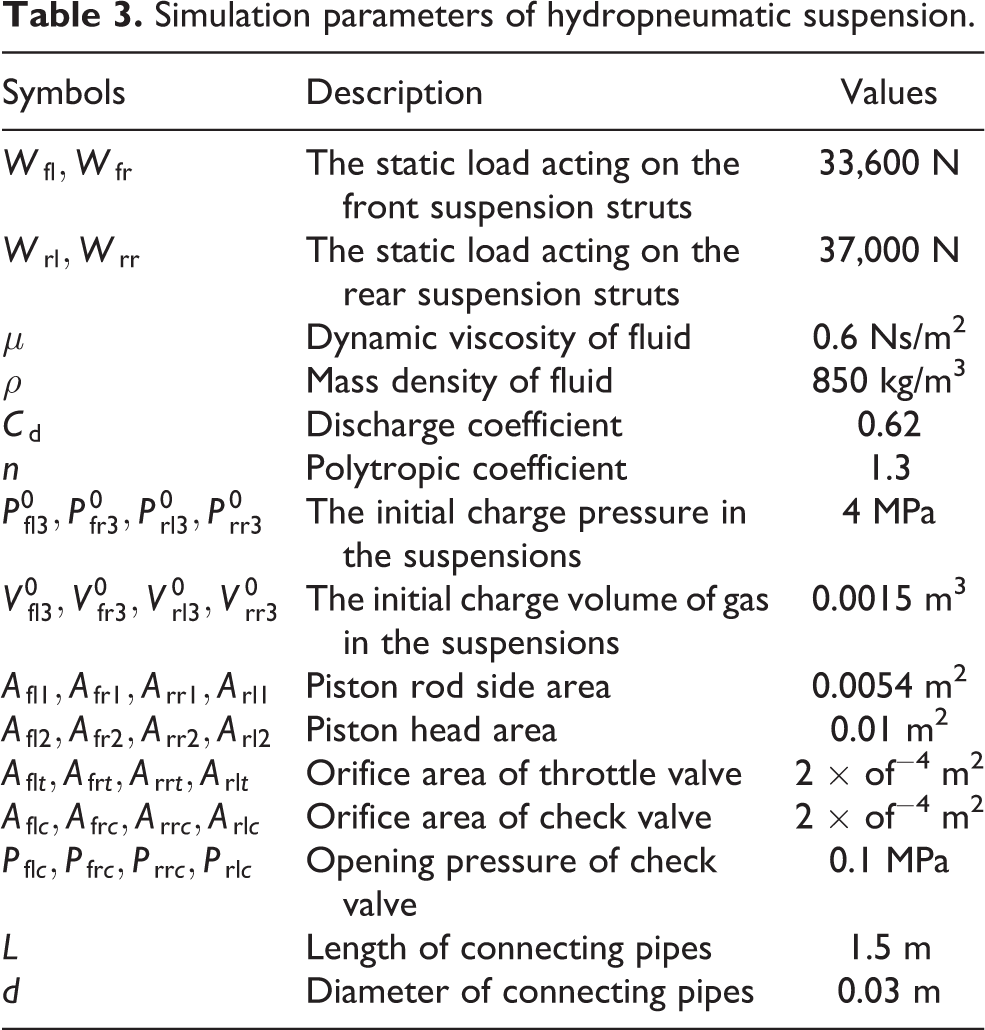
Previous studies have shown that an interconnected hydropneumatic suspension can enhance riding and handling performance. The wheel loader in this study adopts a roll-plane interconnected hydropneumatic suspension (Figure 2), the front-left and the front-right chambers of the struts are interlinked in a cross formation, symmetrically, the rear-left and the rear-right chambers of the struts are also interlinked in a cross formation. Figure 2(b) shows a sample calculation of the interconnected suspension of the suspension forces due to connection symmetry, where the interconnection of the front-left and front-right chambers of the struts is selected to derive the suspension force. The meanings of the symbols in the figure are shown in Table 3. To facilitate the description, the ‘front-left’, ‘front-right’, ‘rear-left’ and ‘rear-right’ are abbreviated as ‘fl’, ‘fr’, ‘rl’ and ‘rr’ in the subscript of the symbols, respectively. For example, F _fl represents the suspension force of the front-left strut.

Figure 2.

Schematic representations of the interconnected hydropneumatic suspension.

Table 3.

Simulation parameters of hydropneumatic suspension.

Symbols	Description	Values
$W_{\text{fl}},W_{\text{fr}}$	The static load acting on the front suspension struts	33,600 N
$W_{\text{rl}},W_{\text{rr}}$	The static load acting on the rear suspension struts	37,000 N
μ	Dynamic viscosity of fluid	0.6 Ns/m2
ρ	Mass density of fluid	850 kg/m3
$C_{\text{d}}$	Discharge coefficient	0.62
n	Polytropic coefficient	1.3
$P_{\text{fl3}}^0,P_{\text{fr3}}^{\text{0}},P_{\text{rl3}}^{\text{0}},P_{\text{rr3}}^{\text{0}}$	The initial charge pressure in the suspensions	4 MPa
$V_{\text{fl3}}^0,V_{\text{fr3}}^0,V_{\text{rl3}}^{\text{0}},V_{\text{rr3}}^{\text{0}}$	The initial charge volume of gas in the suspensions	0.0015 m3
$A_{\text{fl1}},A_{\text{fr1}},A_{\text{rr1}},A_{\text{rl1}}$	Piston rod side area	0.0054 m2
$A_{\text{fl2}},A_{\text{fr2}},A_{\text{rr2}},A_{\text{rl2}}$	Piston head area	0.01 m2
$A_{\text{fl}t},A_{\text{fr}t},A_{\text{rr}t},A_{\text{rl}t}$	Orifice area of throttle valve	2 × of−4 m2
$A_{\text{fl}c},A_{\text{fr}c},A_{\text{rr}c},A_{\text{rl}c}$	Orifice area of check valve	2 × of−4 m2
$P_{\text{fl}c},P_{\text{fr}c},P_{\text{rr}c},P_{\text{rl}c}$	Opening pressure of check valve	0.1 MPa
L	Length of connecting pipes	1.5 m
d	Diameter of connecting pipes	0.03 m

Many previous studies have given mathematical expressions for interconnected hydropneumatic suspensions, ^10,11 the fluid pressure in chambers Ⅰ and Ⅱ of struts fl and fr can be expressed as

$\{\begin{array}{l}{P}_{\text{fl}2}=\frac{\rho }{2C_{\text{d}}^2{A}_{\text{fl}3}^2}{\left(A_{\text{fr}1}{\dot{x}}_{\text{fr}}-A_{\text{fl2}}{\dot{x}}_{\text{fl}}\right)}^2\text{sgn}\left(A_{\text{fr1}}{\dot{x}}_{\text{fr}}-A_{\text{fl2}}{\dot{x}}_{\text{fl}}\right)+P_{\text{fl3}}^{\text{I}}{\left(\frac{P_{\text{fl3}}^0{V}_{\text{fl3}}^0}{P_{\text{fl3}}^0{V}_{\text{fl3}}^{\text{0}}-P_{\text{fl3}}^{\text{I}}\left(A_{\text{fr1}}{x}_{\text{fr}}-A_{\text{fl2}}{x}_{\text{fl}}\right)}\right)}^n\\ P_{\text{fr2}}=\frac{\rho }{2C_{\text{d}}^2{A}_{\text{fr}3}^2}{\left(A_{\text{fl1}}{\dot{x}}_{\text{fl}}-A_{\text{fr2}}{\dot{x}}_{\text{fr}}\right)}^2\text{sgn}\left(A_{\text{fl1}}{\dot{x}}_{\text{fl}}-A_{\text{fr2}}{\dot{x}}_{\text{fr}}\right)+P_{\text{fr}3}^{\text{I}}{\left(\frac{P_{\text{fr}3}^0{V}_{\text{fr3}}^{\text{0}}}{P_{\text{fr}3}^0{V}_{\text{fr3}}^{\text{0}}-P_{\text{fr}3}^{\text{I}}\left({\text{A}}_{\text{fl1}}{\text{x}}_{\text{fl}}-{\text{A}}_{\text{fr2}}{\text{x}}_{\text{fr}}\right)}\right)}^n\\ P_{\text{fl1}}=P_{\text{fr2}}+\frac{A_{\text{fl1}}{\dot{x}}_{\text{fl}}}{K}\\ P_{\text{fr1}}=P_{\text{fl2}}+\frac{A_{\text{fr1}}{\dot{x}}_{\text{fr}}}{K}\end{array}$

1

The fluid pressure in chambers Ⅰ and Ⅱ of struts rl and rr can be expressed as

$\{\begin{array}{l}{P}_{\text{rl2}}=\frac{\rho }{2C_{\text{d}}^2{A}_{\text{rl}3}^2}{\left(A_{\text{rr1}}{\dot{x}}_{\text{rr}}-A_{\text{rl2}}{\dot{x}}_{\text{rl}}\right)}^2\text{sgn}\left(A_{\text{rr1}}{\dot{x}}_{\text{rr}}-A_{\text{rl2}}{\dot{x}}_{\text{rl}}\right)+P_{\text{rl3}}^{\text{I}}{\left(\frac{P_{\text{rl3}}^0{V}_{\text{rl3}}^{\text{0}}}{P_{\text{rl3}}^0{V}_{\text{rl3}}^{\text{0}}-P_{\text{rl3}}^{\text{I}}\left(A_{\text{rr1}}{x}_{\text{rr}}-A_{\text{rl2}}{x}_{\text{rl}}\right)}\right)}^n\\ P_{\text{rr2}}=\frac{\rho }{2C_{\text{d}}^2{A}_{\text{rr3}}^{\text{2}}}{\left(A_{\text{rl1}}{\dot{x}}_{\text{rl}}-A_{\text{rr2}}{\dot{x}}_{\text{rr}}\right)}^2\text{sgn}\left(A_{\text{rl1}}{\dot{x}}_{\text{rl}}-A_{\text{rr2}}{\dot{x}}_{\text{rr}}\right)+P_{\text{rr3}}^{\text{I}}{\left(\frac{P_{\text{rr3}}^0{V}_{\text{rr3}}^{\text{0}}}{P_{\text{rr3}}^0{V}_{\text{rr3}}^{\text{0}}-P_{\text{rr3}}^{\text{I}}\left(A_{\text{rl1}}{x}_{\text{rl}}-A_{\text{rr2}}{x}_{\text{rr}}\right)}\right)}^n\\ P_{\text{rl1}}=P_{\text{rr2}}+\frac{A_{rl1}{\dot{x}}_{rl}}{K}\\ P_{\text{rr1}}=P_{\text{rl2}}+\frac{A_{\text{rr1}}{\dot{x}}_{\text{rr}}}{K}\end{array}$

2

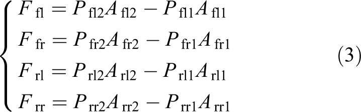
The forces developed by the interconnected hydropneumatic suspension are derived from the forces acting on the pistons

$\{\begin{array}{l}{F}_{\text{fl}}=P_{\text{fl2}}{A}_{\text{fl2}}-P_{\text{fl1}}{A}_{\text{fl1}}\\ F_{\text{fr}}=P_{\text{fr2}}{A}_{\text{fr2}}-P_{\text{fr1}}{A}_{\text{fr1}}\\ F_{\text{rl}}=P_{\text{rl2}}{A}_{\text{rl2}}-P_{\text{rl1}}{A}_{\text{rl1}}\\ F_{\text{rr}}=P_{\text{rr2}}{A}_{\text{rr2}}-P_{\text{rr1}}{A}_{\text{rr1}}\end{array}$

3

The suspension characteristics are based on a set of physical parameters such as static load, charge pressure and volume, orifice area, length and diameter of interconnection pipe. These parameters are presented in Table 3. Each of the parameters are selected based on identical load carrying capacity, static deflection and static stiffness at design ride height. This ensures that the sprung mass natural frequency is within the preferred range for ride quality.

The hydropneumatic suspension is modelled using MATLAB/Simulink (MathWorks, 2012) and provides the RecurDyn full vehicle model with a suspension force via co-simulation, as shown in Figure 3. The RecurDyn vehicle model is linked with Simulink and MATLAB using the RecurDyn/Communicator interface. RecurDyn vehicle model exports the vehicle dynamics variables (velocities and displacements of the cylinder tubes and piston rods) to Simulink. These variables are then used to calculate the suspension forces which are sent back to Recurdyn via Simulink.

Figure 3.

Co-simulation interaction.

Road level identification method based on learning vector quantization neural network

Sample points for neural network training

Learning vector quantization (LVQ) neural network is a forward-supervised neural network with a simple network structure and good pattern recognition characteristics. In this study, it is used to identify road conditions. Sample points for training the neural network are required. These sample points should contain sensitive eigenvalues such as RMS and square root amplitude (SRA) of vertical accelerations which can reflect road surface roughness. Firstly, select sample points of hydrocarbon suspension parameters by using the Latin hypercube method. Next, use the established dynamic model to analyse the vertical accelerations corresponding to these sample points when the wheel loader travels at different speeds on different road levels. Then, calculate the RMS and SRA of the vertical accelerations at the seat position. Lastly, form the neural network training sample points with the travel speed, RMS and SRA of the vertical accelerations as the input and the road level as the output.

The sampling range of hydrocarbon suspension parameters is shown in Table 4. The obtained 30 sample points are shown in Table 5.

Table 4.

Sampling range of design variables.

Variables	Description	Range
P	Initial charge pressure (MPa)	1.5–6.5
V	Initial charge volume (L)	0.5–5
D	Damping hole diameter (mm)	1.5–9

Table 5.

Sample points obtained by the Latin hypercube method.

Sample points	P (MPa)	V (L)	D (mm)	Sample points	P (MPa)	V (L)	D (mm)
1	4.83	4.00	4.66	16	4.26	3.42	3.83
2	4.19	3.17	5.69	17	6.01	4.21	6.18
3	5.13	2.77	3.32	18	5.66	3.50	4.48
4	3.73	4.44	3.64	19	3.92	3.54	4.79
5	2.92	2.67	4.25	20	3.35	4.11	5.52
6	3.62	2.41	3.16	21	2.75	2.89	2.99
7	3.89	3.75	7.89	22	5.66	2.84	6.18
8	5.02	2.99	4.93	23	6.50	2.93	4.31
9	2.59	1.78	3.89	24	5.37	4.83	2.26
10	2.09	3.63	5.08	25	4.36	3.23	4.95
11	4.60	2.57	6.54	26	3.12	2.48	3.44
12	3.18	4.64	5.74	27	2.49	3.08	4.16
13	3.52	2.02	5.97	28	3.46	1.60	2.63
14	4.82	2.28	5.35	29	1.65	0.69	4.07
15	4.05	2.22	2.02	30	4.57	3.33	5.26

P: initial charge pressure; V: initial charge volume; D: damping hole diameter.

The International Organization for Standardization (ISO) has proposed a series of standards of road roughness classification using the power spectral density (PSD) values, as shown in Table 6. The road displacement PSD can be described as

$G(n)=G(n_0){\left(\frac{n}{n_0}\right)}^{-w}$

4

Table 6.

Road roughness values classified by ISO (G(n ₀) × 10⁻⁶).

Road level	Range	Geometric mean
A	8–32	16
B	32–128	64
C	128–512	256
D	512–2048	1024
E	2048–8192	4096

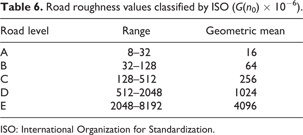
ISO: International Organization for Standardization.

Here, n is the space frequency (m⁻¹) and time frequency f = nv (v is the vehicle speed), n ₀ is the reference space frequency, G(n) is the road displacement PSD, G(n ₀) is road roughness coefficient shown in Table 5, w is the linear fitting coefficient, always w = 2. Based on the standard road surface description, the road surface input model has been built through an inform filter by Gaussian white noise and successfully used in many presented works. ^12,13 The equation of road surface input is

${\dot{z}}_0=-2\pi f_0{z}_0+2\pi \sqrt{G_0{U}_0}{\omega }_0$

5

where f ₀ is low cut-off frequency, G ₀ is road roughness coefficient, ${\omega }_0$ is a Gaussian white noise.

Three types of roads, class C, D and E, are selected as input incentives in this study. Eight different speeds were selected for class C and D roads, that is, 5, 10, 15, 20, 25, 30, 35 and 40 km/h. Only six driving speeds of 5, 10, 15, 20, 25, and 30 km/h were selected on class E road surface due to poor road conditions. The 30 sets of suspension parameter values given in Table 5 will be analysed for the vertical acceleration of the wheel loader at each driving speed. Therefore, a total of 660 sample points for neural network training can be obtained. Select 470 of them as training sample points and 190 sample points as detection points.

The vertical acceleration response corresponding to each sample point was analysed based on the established dynamic model. Sample point 1 was taken as an example when the wheel loader was driving at a speed of 5 km/h on a class C road surface. Figure 4 shows the vertical acceleration response at the seat position. Through the statistical analysis of the acceleration, the RMS value was 198.51 mm/s² and the SRA value is 174.74 mm/s². Similarly, the vertical acceleration RMS values of the other sample points under different conditions could also be obtained.

Figure 4.

Vertical acceleration response at the seat position.

Training LVQ neural network

The LVQ neural network consists of three layers: input, output and hidden. The input layer has three nodes representing the forward speed of the wheel loader, the RMS and the SRA of the vertical acceleration at the seat position. The output layer has a node that represents the level of the road surface. The hidden layer contains eight nodes and a learning rate set to 0.1. Figure 5 shows the results when the LVQ neural network is trained by using the 470 sample points obtained, from which a total of 190 sample points are input into the trained neural network to test the effect of road surface recognition. The number of accurately identified sample points is 172 and the correct rate reaches 90.5%. With C-class road samples taken as an example, only three sample points are identified as D-class road surface.

Figure 5.

Training results of road level recognition.

Parameters optimization and fuzzy controller of hydropneumatic suspension

Parameters optimization of the hydropneumatic suspension of the wheel loader

Establishing the kriging-based surrogate model of the RMS acceleration with respect to the suspension parameters

Establishing the response model of the acceleration RMS with respect to stiffness and damping is complicated due to the non-linear relationship between the vertical acceleration RMS and the suspension parameters. Kriging is a spatial interpolation method based on the geostatistical variogram model. It uses the raw data of the regionalization variables and the structural characteristics of the variogram to optimize the values of the unsampling regional variables. The kriging model has global characteristics rather than local characteristics and is used to predict unknown points based on known points. In this study, kriging method was used to establish the surrogate model between the vertical acceleration RMS and suspension parameters. Then, particle swarm optimization (PSO) algorithm was applied to optimize the parameters of the hydropneumatic suspension to reduce the vertical acceleration and improve ride comfort.

The basic idea of kriging is to predict the value of a function at a given point by computing a weighted average of the known values of the function in the neighbourhood of the point. In design optimization problems, kriging acts as an interpolator, to obtain the value of model response for any intermediate input (design) point within the ‘design variable’ space. The construction of kriging model is a two-stage process. First, a regression function R is built based on the simulated data. Second, a zero mean Gaussian process Z is constructed for the residuals. ¹⁴ A kriging model of response (output) P _k, which depends on a vector of input a, is formulated as

$P_{\text{k}}(a)=R(a)+Z(a)$

6

Further details on the mathematical basis of kriging can be found on books such as the ones by Forrester et al. ¹⁵ and Santner et al. ¹⁶ The kriging module is specially provided in MATLAB, and its main program is as follows: $\text{dmodel=dacefit}(\text{S,Y},@\text{regpoly0,@corrgauss},\theta ,\text{lob,upb)}$ where S represents the obtained 30 sample points of the hydropneumatic suspension and Y denotes the acceleration RMS. The constant regression function and Gaussian correlation equation were selected; θ was the correlation function parameter and was set to [10, 10, 10] in this study; lob and upb indicate the upper and lower limits of the output, respectively.

Parameter optimization analysis of hydropneumatic suspension based on PSO algorithm

In this work, the objective function was defined as the acceleration RMS at the seat position, as shown as follows

$\text{min}f(X)=a_w$

7

where X represents design variables, a _w denotes the RMS acceleration at the seat position and function f is the kriging-based surrogate model.

The design variables were defined as

$X=[P,V,D]$

8

where P is the initial charge pressure, V is the initial charge volume and D is the damping hole diameter.

The suspension deflection was restricted as

${\sigma }_n\le \frac{1}{3}\left[f_d\right]$

9

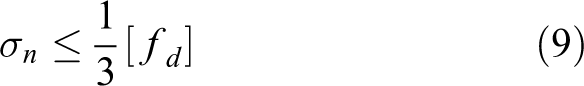
where ${\sigma }_n$ is the RMS of the suspension dynamic deflection, $\left[f_d\right]$ is the dynamic deflection. Wheel loaders belong to heavy vehicles, and the dynamic deflection is often selected as 120 mm. ¹⁷

The tyre dynamic load was restricted as

${\sigma }_{\text{F}z}\le \frac{1}{3}{G}_{\text{F}}$

10

${\sigma }_{\text{R}z}\le \frac{1}{3}{G}_{\text{R}}$

11

where ${\sigma }_{\text{F}z}$ and ${\sigma }_{\text{R}z}$ are the RMS dynamic loads of the front and rear tyres, respectively; and G _F and G _R are the static loads of the front and rear tyres, respectively.

The PSO algorithm was used with the parallel toolbox of MATLAB to optimize the parameters of hydropneumatic suspension for the above-mentioned wheel loader. The number of particles in each swarm was 50, and the loop times were 300. Tables 7 to 9 show the optimization results of the parameters of the hydropneumatic suspension when the wheel loader is running at different speeds on class C, D and E roads.

Table 7.

Optimization results of hydropneumatic suspension parameters when the loader is running on class C road.

Velocity v (km/h)	Initial charge pressure P (MPa)	Initial charge volume V (L)	Damping hole diameter D (mm)
5	3.92	3.56	7.24
10	6.01	4.21	6.18
15	5.13	2.78	7.98
20	4.19	3.18	7.29
25	4.18	3.22	8.49
30	3.35	4.12	7.77
35	3.35	4.07	7.24
40	3.62	2.46	5.67

Table 8.

Optimization results of hydropneumatic suspension parameters when the loader is running on class D road.

Velocity v (km/h)	Initial charge pressure P (MPa)	Initial charge volume V (L)	Damping hole diameter D (mm)
5	3.89	3.75	7.89
10	5.13	2.81	8.51
15	4.57	3.33	8.48
20	5.02	3.02	8.5
25	3.92	3.53	8.56
30	3.9	3.56	7.29
35	4.19	3.14	8.13
40	4.05	2.45	6.42

Table 9.

Optimization results of hydropneumatic suspension parameters when the loader is running on class E road.

Velocity v (km/h)	Initial charge pressure P (MPa)	Initial charge volume V (L)	Damping hole diameter D (mm)
5	4.83	3.98	5.06
10	4.19	3.18	6.58
15	3.92	3.56	6.3
20	4.39	3.67	6.81
25	3.62	2.65	6.63
30	4.26	2.96	6.99

Design of fuzzy controller for hydropneumatic suspension

A fuzzy logic controller involved fuzzification interface, fuzzy rule base, decision-making logic and defuzzification interface. The fuzzification stage will map the real inputs into fuzzy language variables. Then, the fuzzy inference will process the input and calculate the controller outputs according to the control rules. Finally, the outputs are mapped into real control output by the defuzzification stage. In this study, the fuzzy logic controller comprises two inputs, namely, travel speed and road level, while the initial charge volume, initial charge pressure and orifice diameter are the resulting outputs that eventually control the vehicle’s response.

Fuzzification of input and output

Determining the suitable fuzzy controls and membership functions is an important task of a fuzzy controller design. To determine membership functions, the universe of discourse and fuzzy subspaces of travel speed and three controller outputs should be determined first. Here, the active adjustment of suspension parameters is performed based on the road level identification. Each road level corresponds to an independent fuzzy controller. For C-class and D-class roads, the fuzzy domain of the vehicle forward speed is [0,43] and the quantification level is $I_i=\left[5,10,15,20,25,30,35,40\right],I=a,b,\dots h$ . For E-class road surface, the fuzzy domain of the vehicle forward speed is [0,33] and the quantification level is $I_i=\left[5,10,15,20,25,30\right],I=a,b,\dots f$ . Figure 6 illustrates the commonly used triangle and trapezoidal membership functions selected in this study.

Figure 6.

Membership functions of the vehicle forward speed.

The output of the fuzzy controller is the initial charge pressure P, the initial charge volume V and the orifice diameter D. For different road levels, the fuzzy universe of three outputs is as follows:

C-class road: $P_C\in \left[2.7,6.5\right],V_C\in [1.7,4.7],D_C\in \left[5.0,9.0\right]$ .

D-class road: $P_D\in \left[3.6,5.2\right],V_D\in \left[2.4,4.0\right],D_D\in \left[6.0,9.0\right]$ .

E-class road: $P_E\in \left[3,\mathrm{5.2.0}\right],V_E\in \left[2.0,4.4\right],D_E\in \left[4.5,8.0\right]$ .

According to the suspension parameter optimization results shown in Tables 7 to 9, the fuzzy controller output membership functions are established, as shown in Figures 7 to 9. The quantification level of P, V and D corresponding to the class C, class D and class E road surfaces are shown as follows:

Figure 7.

Output membership function for class C road surface: (a) initial charge pressure P, (b) initial charge volume V and (c) orifice diameter D.

Figure 8.

Output membership function for class D road surface: (a) initial charge pressure P, (b) initial charge volume V and (c) orifice diameter D.

Figure 9.

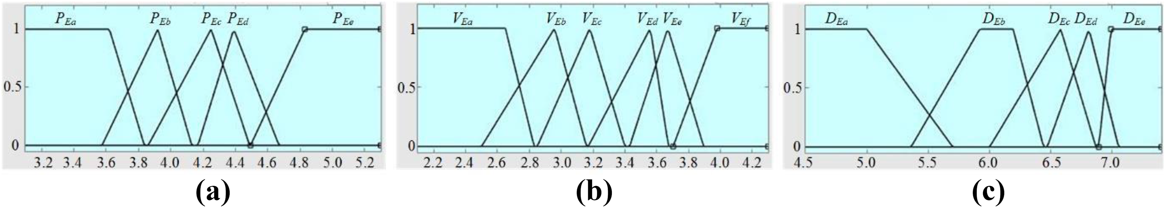
Output membership function for class E road surface: (a) initial charge pressure P, (b) initial charge volume V and (c) orifice diameter D.

C-class road: $P_{Ci}=[3.35, 3.62,3.92, 4.18, 5.13,6.01],V_{Ci}=\left[2.46,2.78,3.18,3.56,4.07,4.21\right],D_{Ci}=\left[5.67,6.18,7.24,7.77,7.98,8.49\right], i=a,b,\dots f$ .

D-class road: $P_{Di}=\left[3.89, 3.92, 4.05, 4.19, 4.57,5.02, 5.13\right], i=a,b,\dots g; V_{Di}=\left[2.45, 2.81,3.02, 3.14, 3.33, 3.53, 3.56, 3.75\right], i=a,b,\dots h; D_{Di}=\left[6.42,7.29,7.89,8.13,8.48,8.56\right],i=a,b,\dots f$ .

E-class road: $P_{Ei}=\left[3.62, 3.92, 4.19, 4.39, 4.83\right],i = a,b,\dots e\text{;} V_{Ei}=\left[2.65, 2.96, 3.18, 3.56,3.67, 3.98\right], i=a,b,\dots f;D_{Ei}=\left[5.06,6.3,6.58, 6.81, 6.99\right],i=a,b,\dots e$ .

The rules of the three kinds of fuzzy controllers corresponding to the three kinds of road levels are described in Table 10.

Table 10.

Fuzzy control rules.

	Ia	Ib	Ic	Id	Ie	If	Ig	Ih
Class C road	PCc /VCd /DCc	PCf /VCf /DCb	PCe /VCb /DCe	PCd /VCc /DCc	PCd /VCc /DCf	PCa /VCe /DCd	PCa /VCe /DCc	PCb /VCa /DCa
Class D road	PDa /VDh /DDc	PDg /VDb /DDe	PDe /VDe /DDe	PDf /VDc /DDe	PDb /VDf /DDf	PDb /VDg /DDb	PDd /VDd /DDd	PDc /VDa /DDa
Class E road	PEe /VEf /DEa	PEc /VEc /DEc	PEb /VEd /DEb	PEd /VEe /DEd	PEa /VEa /DEc	PEc /VEb /DEe

Active control of hydropneumatic suspensions of wheel loaders based on road level identification

Figure 10 shows a flow chart of the active control of hydropneumatic suspension parameters. Firstly, the initial parameters of the hydropneumatic suspension are set, as shown in Table 3, and the different road levels are established. The vertical acceleration at the seat position is calculated based on the established virtual prototyping model of the wheel loader and then statistical analysis is carried out to obtain the RMS and the SRA of vertical accelerations. The statistical analysis frequency is 0.1 Hz. Then, the trained LVQ neural network is used to identify the road level. In this network, the input of the neural network model includes the travel speed, the RMS and the SRA of the vertical acceleration, while the output is the road level. Finally, the identified road level and travel speed are input into the fuzzy control system, which then outputs the adjustment values of the hydropneumatic suspension parameters, namely, charge pressure P, charge volume V and orifice diameter D.

Figure 10.

Control flow chart of hydropneumatic suspension parameters of wheel loaders.

Results and discussion

This study sets three types of road conditions. In the first type of road condition, the wheel loader runs on the C-class road from 0 s to 20 s, on the D-class road from 20 s to 60 s and on the E-class road from 60 s to 100 s, as shown in Figure 11(a). In the second type of road condition, the wheel loader runs on the C-class road from 0 s to 20 s, on the D-class road from 20 s to 60 s and on the C-class road from 60 s to 100 s, as shown in Figure 11(b). In the third type of road condition, the wheel loader runs on the E-class road from 0 s to 20 s, on the D-class road from 20 s to 60 s and on the C-class road from 60 s to 100 s, as shown in Figure 11(c). In all types of road conditions, the loader’s driving speed is 23 km/h.

Figure 11.

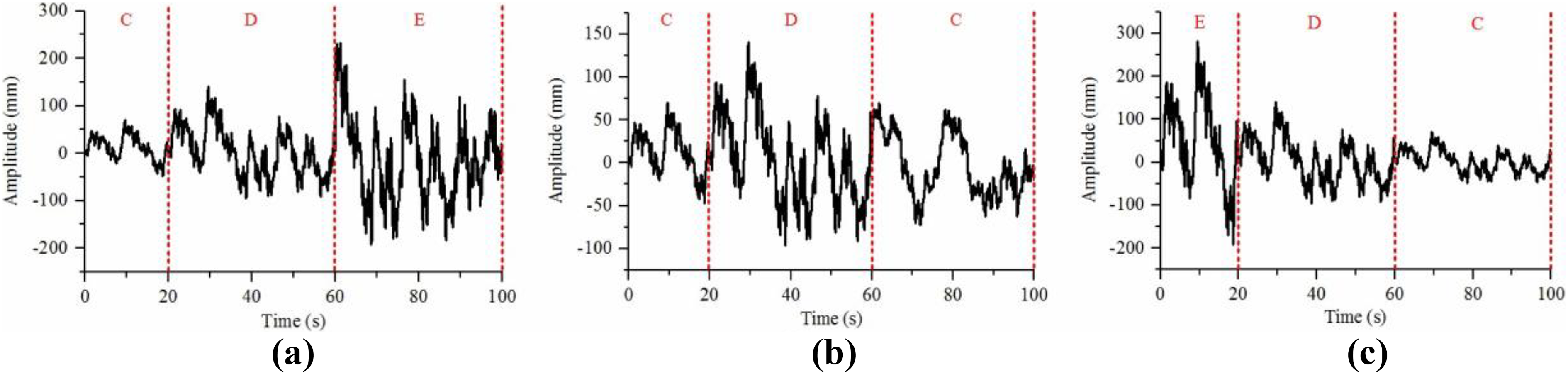
Three types of road conditions: (a) C-D-E, (b) C-D-C and (c) E-D-C.

The established dynamics model is used to simulate and analyse the vertical acceleration at the seat position when the loader travels at a speed of 23 km/h under the first road condition. The RMS and SRA of the vertical accelerations are statistically analysed at 10-s intervals. The statistical results are input to the trained LVQ neural network model to identify the level of the current road. The identification results are shown in Figure 12(a), which reveals that during the entire 100-s simulation analysis process, a total of nine identifications are completed and the recognition results are exactly the same as in the road surface level set in Figure 11(a).

Figure 12.

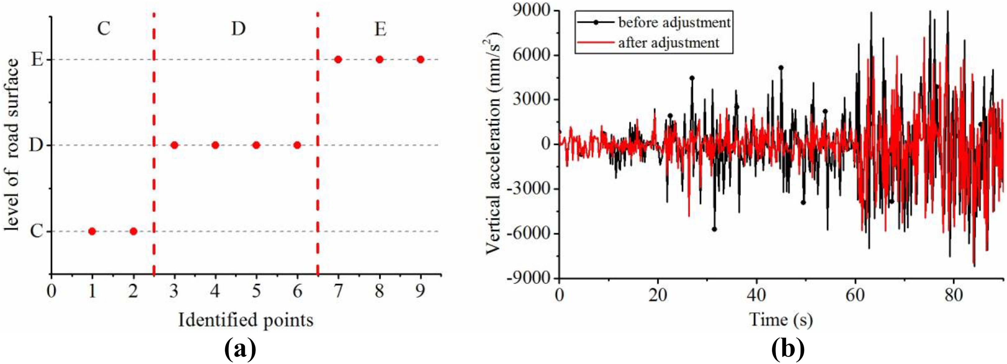
Road identification results and vertical acceleration responses in the first type of road condition.

On the basis of the identified road surface level and vehicle travel speed, the fuzzy controller is used to output the adjustment values of the hydropneumatic suspension parameters. Figure 12(b) shows the vertical acceleration response curve at the seat position before and after the adjustment of suspension parameters. In the initial stage of 0–10 s, the suspension parameters are not yet adjusted because the first recognition of road level is not yet completed. After the first recognition is completed in 10 s, the fuzzy controller actively adjusts the suspension parameters according to the actual road conditions. The active fuzzy adjustment of hydropneumatic suspension parameters on the basis of road level recognition can significantly reduce the vertical acceleration at the seat position. Figures 13 and 14 respectively show the results of road surface level recognition and the vertical acceleration response curve before and after the active adjustment of hydropneumatic suspension parameters under the second and third road conditions. The figures show that the road surface level can be accurately identified and that the active adjustment of hydropneumatic suspension parameters can significantly reduce the vertical vibration.

Figure 13.

Road identification results and vertical acceleration responses in the second type of road condition.

Figure 14.

Road identification results and vertical acceleration responses in the third type of road condition.

Figure 15 shows the comparison of RMS accelerations before and after active adjustment of the suspension parameters. Take the loader runs on the D-class road surface from 20 s to 60 s in the first type of road condition as an example, the RMS of the vertical acceleration is 1811.9 mm/s² when the suspension parameters are not adjusted, drops to 974.7 mm/s² when the suspension parameters are adjusted and decreases by 46.2% before and after the suspension parameters are adjusted. Figure 15 reveals that the RMS of the vertical acceleration decreases by 37%–54% on class C road, by 39%–46% on class D road and by 12%–17% on class D road before and after the suspension parameters are adjusted. Thus, the above analysis indicates that the fuzzy control of hydropneumatic suspension parameters on the basis of road level recognition can effectively improve the comfort of wheel loaders.

Figure 15.

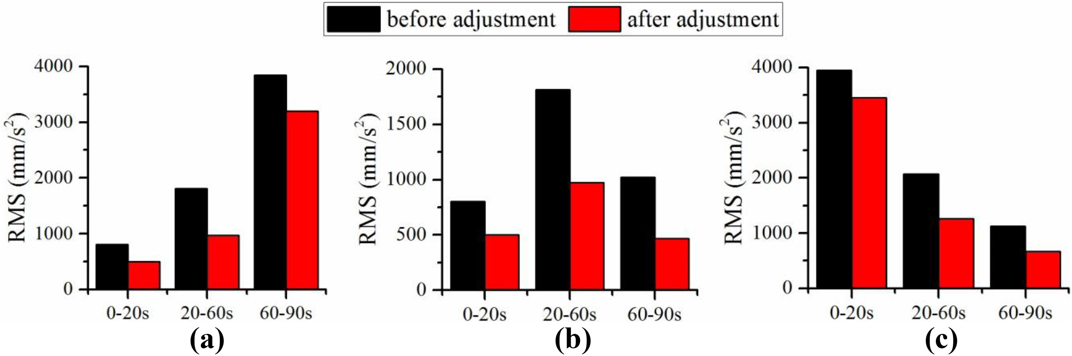
Comparison of RMS accelerations before and after active adjustment of the suspension parameters. RMS: root mean square: (a) C-D-E, (b) C-D-C and (c) E-D-C.

Conclusion

Wheel loaders that travel on unstructured roads experience severe vibration and poor stability. The introduction of suspended axles on wheel loaders, which are traditionally built without wheel suspension, is desirable for ride comfort. A multibody model of a wheel loader with interconnected hydropneumatic suspended wheel axles is developed using the multibody dynamics software RecurDyn. The hydropneumatic suspension is modelled using MATLAB/Simulink, and a RecurDyn full vehicle model with a suspension force is provided via co-simulation. On the basis of these models, this study explores the identification of road levels and the active adjustment of suspension parameters.

A road level recognition method that uses the LVQ neural network is proposed. This method mainly identifies road levels by statistically analysing the RMS and SRA of the vertical acceleration.

The surrogate model of the vertical acceleration RMS with respect to the suspension parameters is established using the kriging method. The optimization model is established with the minimum vertical acceleration as the objective function, the suspension parameters as the optimization variables and the stability of the loader as the constraint condition. The PSO algorithm is used to optimize the model, from which the hydropneumatic suspension parameters that can minimize the vertical acceleration under different loader conditions are obtained.

The fuzzy control rule is formulated based on the optimization results of the hydropneumatic suspension parameters, and a fuzzy controller for the active adjustment of such parameters is designed. The vertical vibration characteristics of the wheel loader when driving on different combinations of roads are analysed, and the results show that the fuzzy control of hydropneumatic suspension parameters on the basis of road level recognition can effectively improve the comfort of the wheel loader.