Sage Journals: Discover world-class research

Abstract

The focus of this study is a moment compensation control algorithm driven by a direct current servo motor. Zero moment robot teaching is achieved with a joint moment compensation algorithm. The moment equilibrium equation is derived based on moment compensation. The current signal detected by a Hall effect sensor is multiplied by a torque constant to estimate the torque value of the robot joint. The compensation current is obtained through parameter identification to overcome gravitational and friction torques. The two variables of speed and position are separately controlled, allowing the compensation current of Coulomb friction and viscous friction force to be separated from the compensation current of friction torque. This study presents the system research, design, and development of a high-precision position control theory of a robot zero moment teaching control method. A collaborative robot is used as the test and verification platform to confirm the feasibility and effectiveness of the proposed theoretical method and implementation technology.

Keywords

Zero moment teaching moment compensation gravity and friction parameter identification collaborative robots

Introduction

A collaborative robot should be able to safely collaborate with people in the absence of guardrails. Traditional industrial robots cannot satisfy this requirement, however this study presents a zero moment control¹ technology based on moment compensation.² It can be applied to the direct teaching of the robot,^3,4 which can eliminate the need for a high-cost multidimensional moment sensor⁵ and make the teaching easy and accurate.

According to current research, robot zero moment control is primarily realized in two ways, zero moment control technology based on position control⁶ and zero force control based on direct moment control.⁷ The foundation of zero moment control technology based on position control is the transformation of the magnitude and direction of external forces into corresponding position commands.^8,9 The servo drive works in the position mode and provides the direct teaching function by tracking the location instruction. There are two ways to obtain the main moment information: one method utilizes sensors, with a six-dimensional moment sensor⁵ at the end of each linkage or torque sensors at all joints to realize detection of an external force, and the second technique is to adopt the method of estimation.^10,11 In the process of robot motion, the value of the Hall effect sensor is converted into the moment minus the moment calculated by the dynamic model.¹² The difference is the magnitude of the estimated external force.

Robot zero moment control

Zero moment control based on position control

Robot zero moment control is based on the robot dynamics model¹³

M (q) \ddot{q} + c (q, \dot{q}) \dot{q} + g (q) + τ_{ext} + τ_{f} = τ_{tot}

In equation (1),

q = generalized coordinate vector of the joint,

$\dot{q}$ , $\ddot{q}$ = velocity and acceleration of each joint, respectively,

M(q) = inertia matrix of the robot (a positive-definite matrix),

$c (q, \dot{q})$ = Coriolis matrix of the robot,

$c (q, \dot{q}) \dot{q}$ = Coriolis and centrifugal forces,

g(q) = gravitation vector, and

τ _tot = sum of all joint torques (rotational joints).

The system of zero moment control technology based on position control is shown in Figure 1.

Figure 1.

Zero moment control system based on force sensor.

In Figure 1, K_p is the position loop gain value of the servo control system, K_v is the speed loop gain value of the servo controller, C_T is the torque constant of the motor, M_g is the gravitational moment corresponding to each joint, M_f is the friction moment corresponding to each joint, M_F is equivalent to the moment of each joint during the contact/collision of the external environment with the robot, q_d is the position signal of each joint, and τ _tot is defined as follows

τ_{tot} = C_{T} K_{v} [K_{p} (q_{d} - q) - \dot{q}]

The position signal value q_d of the motor can be obtained from equation (2)

\begin{array}{l} q_{d} = {K_{p}}^{- 1} ({K_{v}}^{- 1} {C_{T}}^{- 1} τ_{tot} + \dot{q}) + q \\ = {K_{p}}^{- 1} [{K_{v}}^{- 1} {C_{T}}^{- 1} (M_{f} + M_{g} + M_{F}) + \dot{q}] + q \end{array}

The method of zero moment control based on force sensor relates to the technique of estimating the external force value.^14
–16 Its advantages include:

This procedure can detect the magnitude of the external force more precisely. The system is highly sensitive.

With the sensor as the external absolute feedback, there is a higher likelihood of system stability.

Its disadvantages include:

The moment sensor is expensive.

Although joint force sensors will reduce the overall cost of the system compared to the moment sensor, the joint gravity should be allowed for in order to extract the external force information. If using the torque sensor at the end, the end gravity compensation is still required to extract the external force information from the end. The complexity of the system is still high.

It can be predicted that, although the robot will not move too fast in the direct teaching mode, if the robot accelerates greatly, especially a lightweight robot, the torque information detected by the sensor will not be limited to gravity data and may include the inertial force and even the Coriolis and centrifugal forces. In this case, it is difficult to effectively extract the external forces from the composite force information, and the effect of the force sensor is greatly diminished.

The performance of the teaching system is limited by the performance of the sensor, including factors such as temperature drift, sensitivity, and noise resistance.

The advantage of obtaining external force information through estimation is that the cost of the system is reduced due to the lack of sensors. This technique, however, has the following disadvantages:

The accuracy of the external force estimation depends entirely on the accuracy of the dynamic model, and it is very difficult to obtain a precise dynamic model.

The accuracy of the force estimation cannot be guaranteed. Although the dynamic model (rigid body dynamics) can to a large extent reflect the dynamic characteristics of the robot system, the nature of dynamics is to regard the robot system as a second-order physical system. It cannot quantitatively denote mechanical flexibility or the many non-kinetic factors, such as assembly and wear problems. Therefore, if only the dynamic model is used as the fundamental model of external force estimation, the accuracy of the estimated external forces cannot be guaranteed.

The stability of the system is difficult to guarantee because there are no external data available for use as feedback. The system cannot be closed.

Zero moment control based on moment compensation

The method of zero moment control based on direct moment control consists of making the servo drives work in the moment compensation mode by controlling each joint motor’s output moment, in order to overcome the robot’s own gravity and friction. Thus, the robot needs to overcome the smaller inertial forces before moving through external forces. The whole control system can be simply described as shown in Figure 2.

Figure 2.

Zero moment control system based on direct moment control.

Zero moment control technology based on direct moment control requires only the output torque τ _tot of the robot controller. The torque directive is mainly used to overcome the gravitational and friction forces generated by the robot’s mechanical structure. The process is as follows

τ_{tot} = g (q) + τ_{f}

Zero moment control technology based on direct moment control has the following advantages compared to the zero moment control technology based on position control^17,18:

There is no need for force sensors to compensate for gravity and friction, reducing the cost and complexity of the system.

It is not easily affected by the non-dynamic characteristics of the system.

Only a small amount of calculation is required.

The disadvantages mainly include:

Due to the direct control of the torque, the system’s protection of the position and speed loop is weakened, including the emergency stop in the fault state. The system security design is difficult to improve.

The influence of inertia on the robot is obvious. Because the external forces need to overcome the inertial force, for those robots with greater inertia, the necessary external forces will be larger.

Overall, the zero moment control method based on direct moment control greatly reduces system cost and complexity without the need for additional sensors.

Moment compensation based on self-measured gravity and friction

The goal of robot zero moment control is to overcome the effect of robot gravity and friction by compensating for the gravitational and friction moments. The gravitational and friction moments of a robot joint are affected by the joint configuration, load, and motion state of the robot. This study adopts a technique of parameter identification based on the method of least squares. By controlling the rotation speed and angle of the motor separately, an accurate compensation model for Coulomb friction and viscous friction is obtained.

Control system based on direct moment control

To realize zero moment control technology based on direct moment control, the robot control system needs to meet the following requirements:

The driver of each joint of the robot must have an electric current detection module design. The motor drive of each joint is arranged in the tail of the motor, where it is easy to implement wiring and compact design, as shown in Figure 3(a). The Hall effect sensor, also called the Hall sensor, is added to the actuator to detect the current of the joint motor. A Hall sensor is a sensor that uses the Hall effect to transform a large current into a secondary small voltage signal. The Hall sensor is often used to amplify a weak voltage signal into the standard voltage or current signal through the operational amplifier and other circuits, as shown in Figure 3(b).

The robot operator can drag the machine to any position and release it and the machine will not be affected by gravity and friction and thus will remain in the same position.

When the robot is in a normal working state, it will stop immediately and enter zero gravity when there is a collision. At this time, the robot is a flexible mechanism that responds to slight disturbances from the outside world and conforms to the movement trend of external contact forces.

Figure 3.

Electric current detection system of motor driver: (a) Motor driver and (b) Hall effect sensor.

Normally, the robot joint moment needs to be detected by the moment sensor. For a robot that is driven by a direct current (DC) motor, there is a good linear relationship between the electromagnetic torque and the armature current of the DC servo motor.¹⁹ Therefore, the armature current can be used to approximately represent the electromagnetic torque in order to realize moment control. It can reduce the design cost and complexity of the robot by using the current detection method.²⁰

Gravitational moment measurement and compensation

In general, industrial robots must be equipped with torque sensors at each joint or at the end of each linkage to achieve moment control. To satisfy the requirements of low cost and high safety for the collaborative robot, the Hall sensor current detection mode is adopted to replace the traditional detection mode for the moment sensor. To obtain reliable and stable current signals, the drive of each robot joint uses a DC servo motor. Because the electromagnetic torque of a DC servo motor is a linear function of armature current, the moment value of robot joints can be obtained conveniently using the current detection mode. The measured current signal is multiplied by a torque constant, which is the torque value of the robot joint

T = C_{T} I

In equation (5),

T = output torque of the motor,

C_T = torque constant, and

I = detected current of the motor.

After the coordinates of each joint of the robot have been determined, the gravitational moment of each joint has also been determined.

T_{g} = M \cdot f (q)

In equation (6),

T_g = gravitational moment of each joint,

q = generalized coordinates of the joint,

f(q) = vector associated with the robot joint coordinates, and

M = mass matrix of each joint.

In the gravitational moment calculation, the robot joint coordinate vector f(q) is not affected by the robot load, but the mass matrix M of the robot joints is affected. In the real moment compensation algorithm, the actual corresponding mass matrix M is calculated using the load carried by the robot. By substituting the mass matrix M into equation (6), the robot’s gravity moment matrix can be obtained.

Moment control can be achieved by controlling the current. When both sides of equation (6) are divided by the motor torque constant C_T , the following equation is obtained

\frac{T_{g}}{C_{T}} = \frac{M}{C_{T}} \cdot f (q)

The left side of equation (7) is the compensation current for gravity, denoted as I_g , where $I_{g} = T_{g} / C_{T}$ . The right side of equation (7) can be written as $I_{c} \cdot f (q)$ , where $I_{c} = M / C_{T}$ . Thus, equation (7) can be simplified as

I_{g} = I_{c} \cdot f (q)

The constant matrix I_c can be obtained experimentally, as described in the following section. equation (8) yields the amount of current I_g needed to achieve gravitational moment compensation.

Compensation model of gravitational and friction moments: Parameter identification

Compensation model of gravitational and friction moments

When the robot is studied, the constant matrix I_c will eventually be applied to each of its joints. By simplifying the linkage model, stress analysis is carried out by considering the single link established in Figure 4. The measurement method, as well as the accuracy of the measurement of the constant matrix I_c , directly affects the precision of the gravitational moment compensation current I_g .

Figure 4.

Force analysis of the single link.

For a specific joint, the joint motor must be controlled and kept in place. At this point, the current of the motor contains not only sufficient current to overcome the gravity of the joint, but also enough current to overcome friction. The effective current required to overcome gravity and the effective current needed to overcome friction are separately derived from the total measured current.

To simplify the derivation, the single link mechanism shown in Figure 4 can be used to analyze the compensation current. equation (8) can be reduced to the following expression

I_{g} = I_{c} \cdot cos (θ)

It is assumed that I_c is the current required to balance the gravitational moment when the linkage is in a horizontal position (i.e. the horizontal zero position shown in Figure 4). When the rotation angle of the linkage is q = 0, the constant matrix I_c can be measured. Since this is a single linkage, the constant matrix I_c is one dimensional. When the linkage is stable in the horizontal position, the moment balance equation is shown in equation (10)

G_{x} = C_{T} I_{c} + M_{f}

In equation (10),

G = gravity of linkage,

G_x = moment generated by the weight of the linkage itself in the clockwise direction (as shown in Figure 4),

C_T = torque constant,

I_c = current when the linkage is maintained in a horizontal position,

C_TI_c = moment when the linkage is maintained in a horizontal position, and

M_f = friction of the joint. Its direction is uncertain.

equation (10) can be solved, and the actual detection current obtained

I_{c} = \frac{G_{x} - M_{f}}{C_{T}} = \frac{G_{x}}{C_{T}} - \frac{M_{f}}{C_{T}}

From equation (11), it can be seen that the detection current contains the following two inseparable parts: G_x/C_T , the current required to balance the gravitational moment, and −M_f /C_T , the current required to balance the friction moment. The friction moment M_f ∈ [−M_f _max, M_f _max], where M_f _max is the maximum static friction moment of the joint.

The friction moment has a significant influence on the measurement of the gravitational moment. To eliminate interference during the gravitational moment measurement, we designed a specific measurement method to separate the current component generated by the gravitational moment from the test current. For the simplified robot model, the single link mechanism was selected for experimental analysis. The motor was controlled at a constant speed and oscillated at a low speed between two states (1 and 2), as seen in Figure 5. The horizontal position is q ₁ = q ₂; the angle between the two states (1 and 2) is very small, close to 0. Therefore, cos q ≈ 1 and G_x cos q ≈ G_x .

Figure 5.

The motor oscillates from state 2 to state 1.

When the motor oscillates from state 2 to state 1, as shown in Figure 5, the force analysis of the movement process can be obtained

C_{T} I_{2 - 1} = G_{x} cos q + M_{f 1}

The equation for the measured current is obtained by rearranging equation (12)

I_{2 - 1} = \frac{G_{x} cos q + M_{f 1}}{C_{T}} \approx \frac{G_{x} + M_{f 1}}{C_{T}}

In equation (13), M_f ₁ is the friction moment in the clockwise direction.

When the motor moves from state 1 to state 2, as shown in Figure 6, the force analysis of the movement process can be obtained

C_{T} I_{1 - 2} + G_{x} cos q = M_{f 2}

Figure 6.

The motor oscillates from state 1 to state 2.

The equation for the measured current is obtained by rearranging equation (14)

I_{1 - 2} = \frac{M_{f 2} - G_{x} cos q}{C_{T}} \approx \frac{M_{f 2} - G_{x}}{C_{T}}

In equation (15), M_f ₂ is the friction moment in the counterclockwise direction. We can assume that in the entire rotation, the friction in the counterclockwise and clockwise directions is the same, that is, in equations (13) and (15), M_f ₁ = M_f ₂. The average value of the currents measured in equations (13) and (15) is obtained, and the current component generated by the gravity can then be derived

I_{g} = \frac{I_{2 - 1} - I_{1 - 2}}{2} = \frac{G_{x}}{C_{T}}

At the same time, the current component of the force of friction can also be calculated

I_{f} = \frac{I_{2 - 1} + I_{1 - 2}}{2} = \frac{M_{f}}{C_{T}}

Viscous friction and Coulomb friction parameter identification method

The premise used in the derivation of equations (16) and (17) is that the friction moment is the same whether the linkage is rotated in a clockwise or counterclockwise direction. Significantly, there are many factors that affect the friction force, and the friction force is different in different states. Usually, friction can be divided into viscous friction and Coulomb friction. The magnitude of viscous friction is proportional to velocity; its value is 0 when the velocity is 0. Coulomb friction is proportional to the normal load, which is opposite to the direction of motion and is not dependent on the contact area.

Since viscous friction is proportional to speed, in the viscous friction parameter identification method, we can control the oscillation speed, keep other conditions unchanged, and record the changes of the current at different speeds. The experimental platform is shown in Figure 7. The load at the end of the linkage is 562 g.

Figure 7.

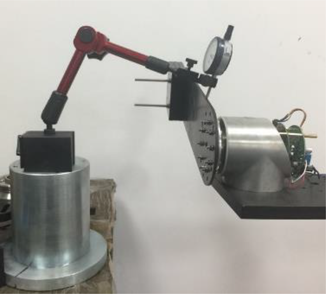
Friction parameter identification experimental platform.

Figure 8 shows the experimental results. The joint speed increased from 1 r/min to 41 r/min. With this increase of rotational speed, the current of the viscous friction moment increased slightly. After the rotational speed reached 20 r/min, the current values stayed nearly constant at 1.7 A for counterclockwise rotation and 1.4 A for clockwise rotation. This shows that when the velocity reaches a certain value, viscous friction is no longer affected by velocity. The average value of the current at different rotation speeds is the corresponding current of the viscous friction. Based on the analysis of the experimental results and MATLAB [version R2016b] simulation, cubic spline interpolation curves were used to fit the current generated by the friction force at different speeds. The resulting equation was

I_{v} = p_{1} v^{3} + p_{2} v^{2} + p_{3} v + p_{4}

In equation (18),

I_v = current component of viscous friction,

v = velocity, and

p ₁, p ₂, p ₃, p ₄ = parameters need to be identified.

Figure 8.

The current that corresponds to viscous friction.

The model parameters p ₁, p ₂, p ₃, and p ₄ were identified using the method of least squares. The parameter identification is shown in Figure 9; the results met the fitting requirements.

Figure 9.

Parameter identification of the current got at different speeds. The calculated results of the parameters p ₁, p ₂, p ₃, and p ₄ are 0.1276, −0.248, 0.06986, and 1.581, respectively. At the same time, the SSE = 0.04398 is very close to 0 and the coefficient of determination, R ² = 0.9835, is very close to 1. These values indicate that the model selection and fitting are good and the data prediction is successful. SSE: sum of squares due to error.

Coulomb friction is only proportional to the normal load. The parameter identification method for Coulomb friction consists of rotating the joint to different positions so that it experiences different normal loads. In addition, the current was recorded in both counterclockwise and clockwise directions at each position ranging from 0° to 90°, in intervals of 4.5°. The current is required to realize oscillation at a low speed. The test results are shown in Table 1.

Table 1.

Oscillating current at all angles.

Position, q (°)	Counterclockwise current, I _2–1 (A)	Clockwise current, I _1–2 (A)	Average current, I (A)	Current of Coulomb friction, I (A)	Position, q (°)	Counterclockwise current, I _2–1 (A)	Clockwise current, I _1–2 (A)	Average current, I (A)	Current of Coulomb friction, I (A)
0	0.453	0.325	0.3890	0.128	49.5	0.311	0.230	0.2705	0.081
4.5	0.434	0.313	0.3735	0.121	54	0.306	0.225	0.2655	0.081
9	0.428	0.308	0.3680	0.120	58.5	0.300	0.220	0.2600	0.080
13.5	0.420	0.303	0.3615	0.117	63	0.295	0.218	0.2565	0.077
18	0.410	0.297	0.3535	0.113	67.5	0.283	0.209	0.2460	0.074
22.5	0.401	0.289	0.3450	0.112	72	0.275	0.203	0.2390	0.072
27	0.392	0.284	0.3380	0.108	76.5	0.264	0.193	0.2285	0.071
31.5	0.380	0.276	0.3280	0.104	81	0.258	0.189	0.2235	0.069
36	0.360	0.263	0.3115	0.097	85.5	0.247	0.180	0.2135	0.067
40.5	0.341	0.249	0.2950	0.092	90	0.238	0.175	0.2065	0.063
45	0.324	0.238	0.2810	0.086

As can be seen from Table 1, for each joint position, the measured value of the current for the counterclockwise direction differs from that of the clockwise direction. The fifth column in Table 1 is the current generated by Coulomb friction in the current joint position. This can be calculated by subtracting the clockwise current (third column) from the counterclockwise current (second column).

According to the data in the fourth and fifth columns of Table 1, the relationship between average current and Coulomb friction current can be obtained, as shown in Figure 10. The average current has a generally linear relation to the Coulomb friction current, though not perfectly linear. Based on the analysis of the experimental results and MATLAB simulation, quadratic spline interpolation curves were used to fit the Coulomb friction current with the detection current. Since the fit was very good, the following assumption was made

I_{co} = a I^{2} + b I + c

In equation (19),

I _co = current generated by Coulomb friction,

I = detection current, and

a, b, c = parameters need to be identified.

Figure 10.

The average current and the Coulomb friction current.

The model parameters a, b, and c were identified using the method of least squares. The parameter identification is shown in Figure 11; the results met the fitting requirements.

Figure 11.

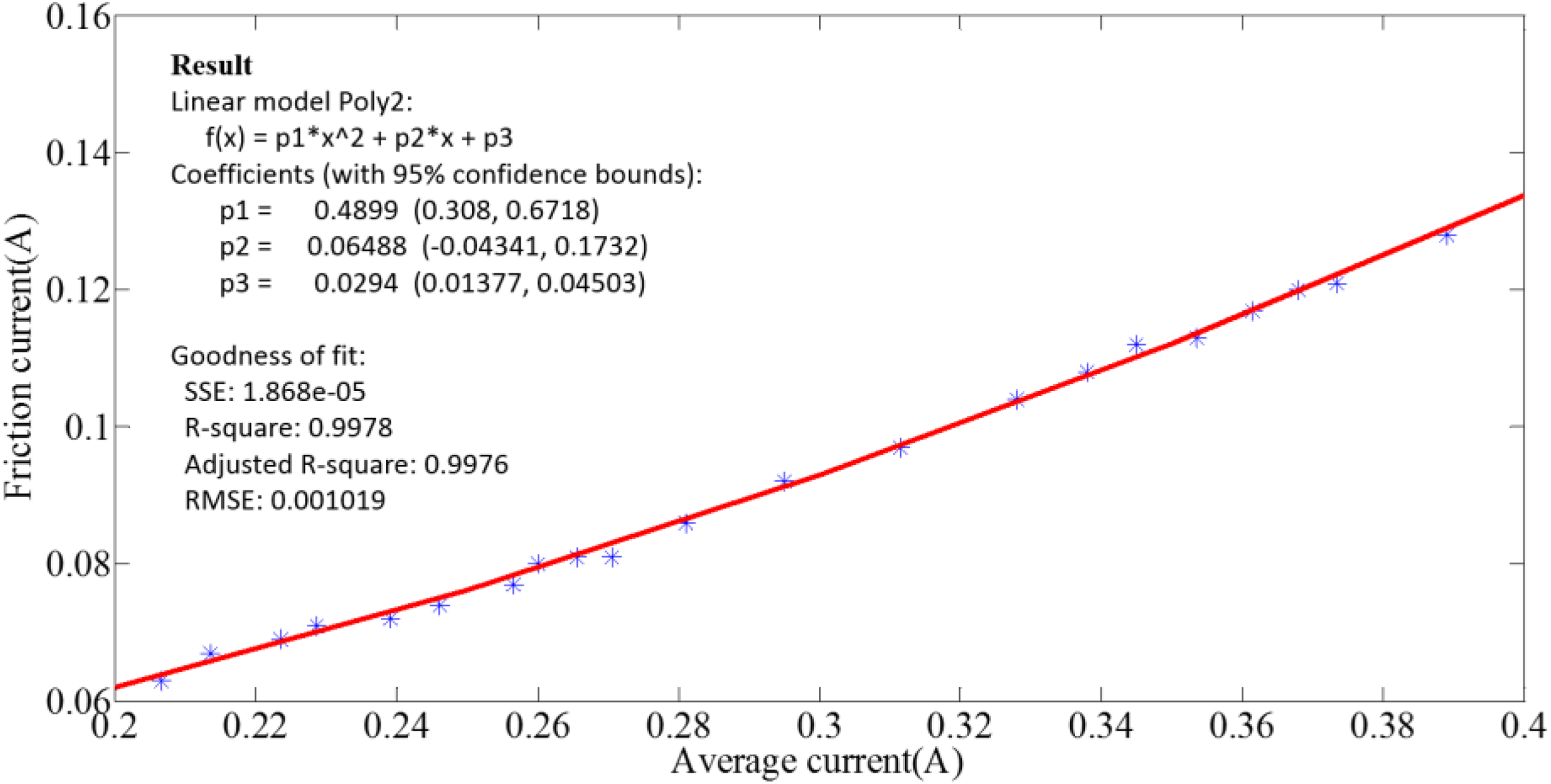
Parameter identification of the Coulomb friction current. The SSE = 1.868 × 10⁻⁵ is very close to 0 and the coefficient of determination R ² = 0.9978 is very close to 1. These values indicate that the model selection and fitting are good and the data prediction is successful. SSE: sum of squares due to error.

Moment compensation control algorithm

The compensation current corresponding to the gravitational and friction moments is deduced using the procedure described in the “Compensation model of gravitational and friction moments: Parameter identification” section. To realize zero force control mode during joint rotation, it is necessary to overcome the currents of the gravitational and friction moments (Coulomb friction and viscous friction, respectively).

I_{s} = I_{g} + I_{v} + sgn (\dot{q}) I_{co}

equation (20) is the current compensation model for the moment compensation control algorithm, where $sgn (\dot{q})$ indicates that the direction of Coulomb friction is opposite to the direction of relative movement. I_g can be obtained from equation (14), I_v can be obtained from equation (16), and I_c can be obtained from equation (17).

For multi-degree-of-freedom (multi-DOF) robots, friction parameters identification of each joint is required. The robot system model with viscous friction and Coulomb friction is based on equations (16) and (17), and the parameters that need to be identified in the model are obtained through simulation calculation. After the viscous friction and Coulomb friction have been calculated, the moment compensation model is determined. The final current compensation of the gravitational and friction moments is then calculated using equation (18). Errors in the experimental process are unavoidable. In addition, the robot model has been simplified to a single linkage model, which cannot accurately represent the actual state of the robot. Therefore, the actual compensation model must leave an appropriate allowance for the improvement of system stability.

When teaching at a low speed, the compensation current calculated by the moment compensation control algorithm can overcome the gravitational and friction torque of the robot perfectly and make the robot in the mode of zero moment, so the user can easily drag the robot.

However, in the actual teaching process, it is inevitable that the teaching speed is too fast. At this point, due to the influence of the counter electromotive force of the motor, the compensation current calculated by the moment compensation control algorithm cannot meet the requirements of the teaching process of the robot. At this point, the compensation current value meets the following requirements

I_{c} = I_{s} - \frac{K_{b} w}{R_{m}}

In equation (21),

K_b = counter electromotive force of the motor,

w = angular velocity of the motor, and

R_m = resistance of the motor.

The compensation current obtained by equation (21) can satisfy the teaching of the robot at any speed and make the whole system of the robot more stable.

Experiment

A collaborative robot JITRI5 contributed by our group was used to verify the feasibility and effectiveness of the zero moment control algorithm. It has six DOFs. Each joint of the robot adopts the hollow torque brushless motor, hollow harmonic driver, hollow shaft, hollow encoder, and so on. This design can make the robot more light and easy for wiring.²¹ As seen in Figure 12, it shows the joint structure of JITRI5.

Figure 12.

The joint structure of JITRI5. TBM: torque brushless motor.

The experimental platform is shown in Figure 13. There were two kinds of joints in the robot. Joints 1–3 consisted of one type and joints 4–6 consisted of the other type. The motors of the joints are shown in Table 2. To reflect the advantage of zero moment teaching, a weight of 1937 g was loaded at the end of the final linkage in the robot. In the experiment, two current data were collected through the Hall current sensor when the robot moved with and without the moment compensation mode.

Figure 13.

The experimental platform of the collaborative robot JITRI5.

Table 2.

Motor selection.

Joint	Motor type	Rated torque (N m)	Rated power (W)	Rated speed (r/min)
Joints 1–3	TBM(S)-7615-X	0.996	280	4025
Joints 4–6	TBM(S)-6013-X	0.413	117	4300

TBM: torque brushless motor.

It is difficult for the robot to implement teaching when there is no moment compensation mode, especially when bearing a load.²² It is necessary to overcome the gravity and friction of the robot during the teaching process. When the gravitational and friction moment compensations are added, the teaching force will be greatly reduced, and the robot joint can be easily pulled by overcoming the inertial force generated by the joint rotation. When the robot adopted the moment compensation mode, the current change of joint 2 was most obvious, as shown in Figure 14. The red dashed line shows the current of joint 2 when the robot was teaching in the moment compensation mode. The solid black line shows the current of joint 2 when the robot did not use the moment compensation mode. The compensation current of the joint was calculated according to equation (21). It can be seen from the figure that the compensation current needed for teaching the robot differed for different positions. The required compensation current was lowest when the robot was in the vertical state and highest when the linkage was dragged to the horizontal state (time = 10 s in the figure). After 15 s, the robot was dragged back to the vertical state and the magnitude of the compensation current decreased. After 22 s, the robot performed repetitive motions and the magnitude of the compensation current increased. When the robot was dragged back to the vertical state, the magnitude of the compensation current decreased. From the data, we can see that the robot moved from the vertical state to the horizontal state twice.

Figure 14.

The current of joint 2 in the teaching.

Conclusions

In this article, a zero moment control model was established on the basis of the dynamic model. By overcoming the gravitational and friction moments of the robot, the current compensation was obtained. During experimental analysis, the method of least squares was adopted for the parameter identification of the coefficients of Coulomb friction and viscous friction. Using this method, an accurate compensation model was obtained.

The proposed zero moment control algorithm based on moment compensation differs from traditional zero moment control technology based on position control. In the teaching process of the robot, the proposed method can calculate and compensate for the current caused by the gravitational and friction moments in real time. The robot is easy to teach by overcoming its inertial force.

Using a simplified linkage model and the results of the experiment, the gravitational and friction moments of the linkage were identified. The current model was generated from the gravitational and friction moments. The current compensation control algorithm was used for zero moment control.

A test of the proposed control algorithm was performed which showed that the robot was still easy to teach when the end of the linkage was loaded with a weight of 1937 g. The experimental results showed that the compensation effect of the zero moment control algorithm based on moment compensation is obvious, which makes the teaching process easier.

Compared with the traditional zero moment control algorithm based on position control, the zero moment control algorithm based on moment compensation control eliminates the expensive torque sensor. This method can be used to convert the detection current into the moment, which simplifies the entire robot system, reduces the cost of the robot, and makes the teaching process easier and more flexible. A new approach was also presented to control collaborative robots.

Footnotes

Declaration of conflicting interests

The author(s) declared no potential conflicts of interest with respect to the research, authorship, and/or publication of this article.

Funding

The author(s) disclosed the receipt of following financial support for the research, authorship, and/or publication of this article: This study was supported by the fund of Key Research and Development Plan of Jiangsu Province (item number: BE2017603), and it is verified by the Robot Laboratory of the Service Robot Laboratory of the Institute of Intelligent Manufacturing Technology of Jiangsu Institute of Industrial Technology Research Institute.

ORCID iD

Saixuan Chen

Omar Abdelaziz

References

Santiago

Garcia-Haro

Victores

. Experimental robot model adjustments based on force–torque sensor information. Sensors 2018; 18: 836. DOI: 10.3390/s18030836.

Lai

Yang

Jin

. Novel measurement method for determining mass characteristics of pico-satellites. Appl Sci 2018; 8: 104. DOI: 10.3390/app8010104.

Fernando

Zalewski

. Teaching joint-level robot programming with a new robotics software tool. Robotics 2017; 6(4): 41. DOI: 10.3390/robotics6040041.

Lin

. A novel teaching system for industrial robots. Sensors 2014; 14(4): 6012–6031. DOI: 10.3390/s140406012.

Likun

Dong

. Probabilistic sensitivity amplification control for lower extremity exoskeleton. Appl Sci 2018; 8(4): 525. DOI: 10.3390/app8040525.

Wei

Sun

Wang

. Nonlinear state feedback position control for flexible joint robot with energy shaping. Robot Auton Syst 2018; 99: 121–134.

Lei

Yin

Wang

. Position control for flexible joint robot based on online gravity compensation with vibration suppression. IEEE Trans Ind Electron 2018; 65(6): 4840–4848.

Ansari

Manti

Falotico

. Multiobjective optimization for stiffness and position control in a soft robot arm module. IEEE Robot Autom Lett 2018; 3(1): 108–115.

Komal

Kumar

. Design of intelligent hybrid force and position control of robot manipulator. In: The 6th international conference on smart computing and communications (eds Mathew

Singh

), Kurukshetra, India, 7–8 December 2017, pp. 42–49. Elsevier.

10.

De Luca

Albu-Scha¨ffer

Haddadin

. Collision detection and safe reaction with the DLR-III lightweight manipulator arm. In: IEEE/RSJ international conference on intelligent robots and systems, Beijing, China, 9–15 October 2006, pp. 1623–1630. IEEE.

11.

Haddadin

Albu-Schaffer

De Luca

. Collision detection and reaction: a contribution to safe physical human-robot interaction. In: IEEE/RSJ international conference on intelligent robots and systems, Nice, France, 22–26 September 2008, pp. 3356–3363. IEEE.

12.

Cho

Hong

Kim

. Neural network based adaptive actuator fault detection algorithm for robot manipulators. J Int Robot Syst. Epub ahead of print 31 January 2018. DOI: 10.1007/s10846-018-0781-0.

13.

De Luca

Mattone

. Sensorless robot collision detection and hybrid force/motion control. In: Proceedings of the IEEE international conference on robotics and automation, Barcelona, Spain, April 2005, pp. 999–1004. IEEE.

14.

Jin

Xiong

. Contact force estimation for robot manipulator using semiparametric model and disturbance Kalman filter. IEEE Trans Ind Electron 2018; 65(4): 3365–3375.

15.

Yeping

Liao

. Existence and zero-electron-mass limit of strong solutions to the stationary compressible Navier-Stokes-Poisson equation with large external force. Math Methods Appl Sci 2017; 4634: 646–663. DOI: 10.1002/mma.

16.

Zhenyu

Huang

Liu

. Predictive approach for sensorless bimanual teleoperation under random time delays with adaptive fuzzy control. IEEE Trans Ind Electron 2017; 65(3): 2439–2448.

17.

Lascu

Boldea

Blaabjerg

. A modified direct torque control (DTC) for induction motor sensorless drive. In: Thirty-third IAS annual meeting industry applications conference, 1998, St. Louis, MO, USA, 12–15 October 1998, pp. 415–422. DOI: 10.1109/IAS.1998.732336.

18.

Davari

Rodriguez

. Predictive direct voltage control of induction motor with mechanical model consideration for sensorless applications. IEEE J Emerg Sel Top Power Electron. Epub ahead of print 13 March 2018. DOI: 10.1109/JESTPE.2018.2815652.

19.

Schagin

. Implementation of data driven control system of DC motor by using system identification process. In: IEEE conference of Russian young researchers in electrical and electronic engineering (EICon-Rus), Moscow, Russia, 29 January–1 February 2018, pp. 1801–1804. IEEE.

20.

Cornell

Johnson

Peck

. Design of a modular snake robot. In: IROS 2007, IEEE/RSJ international conference on intelligent robots and systems, San Diego, CA, USA, 29 October–2 November 2007, pp. 2609–2614. IEEE.

21.

Lee

Song

. Design of a 6-DOF collaborative robot arm with counterbalance mechanisms. In: Proceedings–IEEE international conference on robotics and automation, Singapore, 29 May–3 June 2017, pp. 3696–3701. IEEE.

22.

Villani

Pini

Leali

. Survey on human-robot collaboration in industrial settings: safety, intuitive interfaces and applications. Mechatronics. Epub ahead of print 2 March 2018. DOI: 10.1016/j.mechatronics.2018.02.009.

Collaborative robot zero moment control for direct teaching based on self-measured gravity and friction

Abstract

Keywords

Introduction

Robot zero moment control

Zero moment control based on position control

Zero moment control based on moment compensation

Moment compensation based on self-measured gravity and friction

Control system based on direct moment control

Gravitational moment measurement and compensation

Compensation model of gravitational and friction moments: Parameter identification

Compensation model of gravitational and friction moments

Viscous friction and Coulomb friction parameter identification method

Moment compensation control algorithm

Experiment

Conclusions

Footnotes

Declaration of conflicting interests

Funding

ORCID iD

References