
Abstract
For when a structure is both subjected to unknown loads and characterized by unknown parameters and structural parameter identification and load identification algorithms cannot be applied under these circumstances, this article proposes a new algorithm based on the perturbation method for the simultaneous identification of the load and unknown structural parameters using a few response points. The impulse response matrix is expanded with respect to the unknown parameters, and then the load term is combined with the unknown parameter perturbation term to generate the parameter–load term; finally, the load and unknown parameters can be simultaneously identified by iteration. The proposed algorithm is verified by an example of a 10-storey shear frame, and the effect of noise level, the number of response points, and the truncation ratio, which is a parameter introduced to improve the accuracy of the proposed algorithm, are studied. Moreover, the effect of the distribution of response points is discussed for another example of a simply supported beam, and the results show that when the response points are distributed over the full beam, the error is obviously smaller than when the response points are distributed over only part of the beam.
Keywords
Introduction
Civil engineering structures have been subjected to environmental and human loads during many decades of operation, which may cause damage to the structures, thereby changing the structural parameters. The structural vibration response is a direct representation of the structural parameters. Many damage identification algorithms 1 determine the position and size of the damage by estimating the changes in parameters. Therefore, it is a significant research direction to monitor the response of the structure and then obtain the structural parameters using the response to evaluate the current structural security situation.
Traditional structural parameter identification algorithms require the input and output of the structure to obtain the frequency response function in frequency domain or impulse response function in time domain to identify structural parameters, which is obviously difficult to realize in most cases. The structural parameter identification algorithms based on environmental excitation 2 do not require structural input, for example, time series analysis, 3 natural excitation technique (NExT), 4 and stochastic subspace identification (SSI), 5 but the accuracy of structural parameter identification algorithms decreases, and even the algorithms may fail when the external load does not satisfy the Gaussian distribution assumption. For structural dynamic load identification algorithms, 6 it is necessary to know all the parameter information of the structure accurately in advance. However, some structural parameters cannot be easily obtained, especially after the structure is damaged.
Considering that a structure has both unknown loads and unknown parameters, if the unknown loads can be identified simultaneously with the unknown structural parameters, not only can the structural safety condition be evaluated by comparison of the identified structural parameters and the initial design parameters, but also the load source can be roughly determined according to the time history of the identified load. Meanwhile, more appropriate measures can be taken to control the load source or change the transmission path of the load to reduce the structural response, which can effectively lower the risk to the structure to ensure its long-term stable and safe operation.
In recent years, only the use of structural dynamic response to identify loads and unknown parameters has gradually developed. The most common algorithms are based on least-squares method7–10 or Kalman filtering.11–14 Moreover, Zhu and Law 15 identified the damage of a concrete bridge under moving load, and the interaction forces between the vehicle and the bridge are also identified simultaneously. A damage function is adopted to simulate the crack damage. Lu and Law 16 proposed a composite algorithm based on the sensitivities of response with respect to the load and unknown parameters. Zhang et al.17,18 solved the problem of the composite identification of the load and parameters based on the virtual distortion method (VDM). Huang et al. 19 developed a new algorithm, referred to as the adaptive quadratic sum–squares error with unknown excitations (AQSSE-UI) by minimizing the quadratic sum–squares error between the measured response and the theoretical values. Law and Ding 20 proposed two sub-structural identification methods with the structure divided into substructures and with one substructure assessed at one time. Sun and Betti 21 presented a hybrid heuristic optimization strategy based on the artificial bee colony (ABC) algorithm with a local search operator. Feng et al. 22 proposed a new method to identify structural parameters and vehicle dynamic axle loads of a vehicle–ridge interaction system in the framework of an iterative parametric optimization process. A Bayesian inference regularization is presented to solve the ill-posed least-squares problem. Pioldi and Rizzi 23 proposed a new element-level system identification and input estimation technique named full dynamic compound inverse method (FDCIM). A statistical average technique, a modification process, and a parameter projection strategy are adopted at each stage to achieve stronger convergence. Jayalakshmi and Rao 24 used a newly developed dynamic hybrid adaptive firefly algorithm (DHAFA) to solve the inverse problem associated with the system identification.
Based on the perturbation theory, this article proposes a new algorithm for simultaneous identification of the load and unknown parameters of the structure using a few response points. First, initial values are assumed for unknown parameters, and the convolution equation for solving the structural dynamic response is discretized. Next, the impulse response matrix is expanded with respect to unknown parameters at the assumed initial values. The partial derivative matrices of the impulse response matrix with respect to the unknown parameters are obtained by the difference method. The load term is combined with each unknown parameter perturbation term to generate the parameter–load term, and then the load term and the parameter–load term can be determined by inversion with Tikhonov regularization method 25 and L-curve criterion. 26 Each unknown parameter perturbation term is calculated using the ratio of the norm of the corresponding parameter–load term to that of the load term, and its positive and negative proprieties are determined by the method proposed in this article. Subsequently, all unknown parameter perturbation terms are added to initial values, and the resulting values are treated as the new initial values. Finally, the next iteration step proceeds until the identified results converge. In an example of a 10-storey shear frame structure, the effect of the number of response points, noise level, and truncation ratio on the identified results are studied. The proposed algorithm is also applied to the identification of another example of a simply supported beam under the action of a concentrated load, and the effect of the distribution of response points is also discussed.
Simultaneous identification of the load and unknown parameters
For a single-degree-of-freedom system with damping, the equation of motion can be written as

in which, m, c, and k are the mass, damping, and stiffness, respectively;
Suppose that both the initial velocity and the initial displacement are zero, then the convolution equation for solving the structural displacement response can be obtained by Duhamel integral

in which
Let

in which
Similarly, for a N-degrees-of-freedom system with proportional damping, the equation of motion can be written as

in which
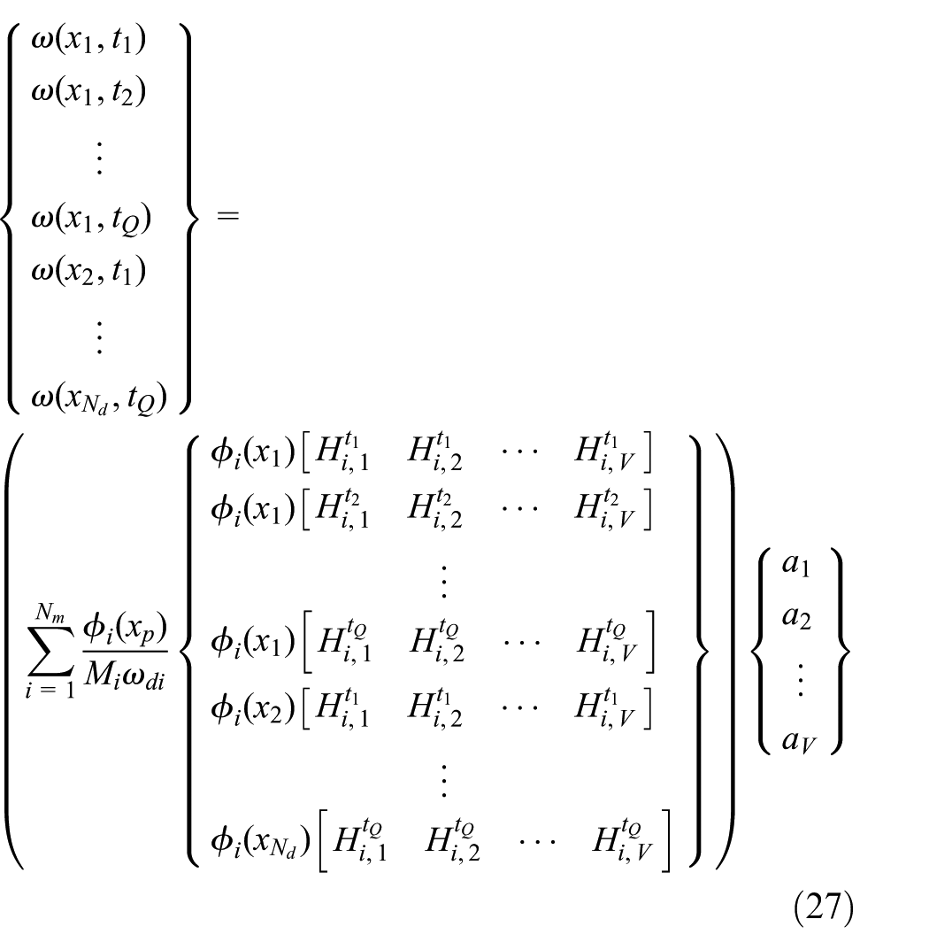
Suppose that the initial velocity and the initial displacement vectors are zero. Using the orthogonality of the mass matrix, stiffness matrix, and damping matrix with respect to the mode shape matrix, the displacement of the selected response points calculated by the superposition method is discretized according to time sampling points as in equation (3)
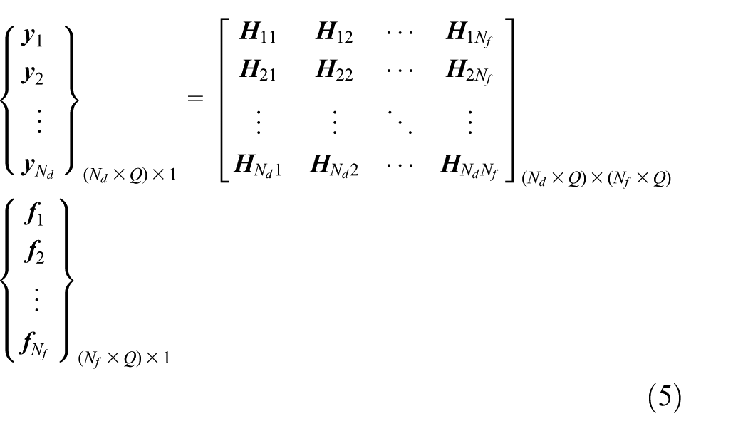
in which
It is assumed that the structure contains l unknown parameters, which can be expressed as

in which the superscript “T” represents the matrix transposition.
Equation (5) can be simplified into the following form containing the unknown parameters

According to the perturbation theory, first, the initial values are assumed for all unknown parameters, and then the impulse response matrix
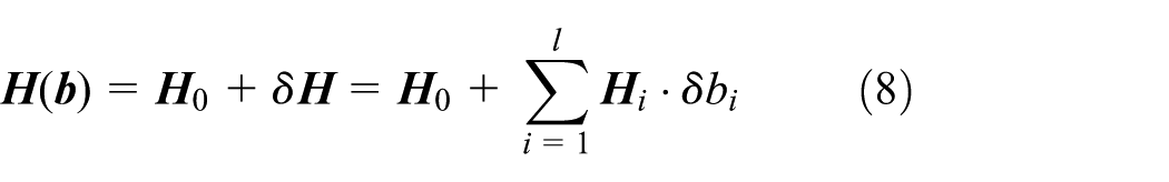
in which
Substituting equation (8) into equation (7), one can obtain

Combining the ith unknown parameter perturbation term

Solving the generalized inverse of equation (10), the load term and parameter–load term can be obtained

in which the superscript “+” represents the generalized inverse.
Then, the ith unknown parameter perturbation term can be determined using the ratio of the norm of

in which |·| represents the absolute value, and
The absolute value of an unknown parameter perturbation term is given for the reason that the ratio of the norm of
Suppose that the load term

Next, the elements in
First,
After the perturbation terms are determined, they are added to the initial values of the unknown parameters, and then the results are taken as the initial values in the next iteration step, until the identified results converge.
In addition, for a multiple-degrees-of-freedom structure, it is difficult, even impossible to obtain the explicit expression of the impulse response function with respect to a certain structural parameter. Therefore, the difference method is used. Specifically, suppose that an unknown parameter has a small perturbation at its initial value; then, the discrete impulse response functions are calculated before and after the occurrence of the perturbation, and the difference between the two impulse response functions is treated as the partial derivative of the impulse response function with respect to this unknown parameter.
Introduction of the orthogonal polynomials
It can be seen from equation (7) that when the load and unknown parameters are simultaneously identified, the number of unknown terms becomes

in which
The load term

in which
Substituting equation (15) into equation (10), one can obtain

In general, it is usually sufficient to use a few orthogonal polynomials to accurately reconstruct the load, and thus, the number of unknown terms that must be identified is greatly reduced, enabling the identification of the load and unknown parameters using fewer response points. Therefore, it is difficult to apply this algorithm to the identification of an impact load or a random load.
Regularization and selection of the regularization parameter
Because of the inevitable ill-condition of the matrix

in which
After the regularization parameter is determined, the least-squares method is used to obtain the unknown sequence

in which
Next, the sequence
In the case of calculating the partial derivative matrix of unknown parameters in equation (8), it is necessary to take a very small perturbation step to ensure the accuracy of the final identified results, which also leads to the fact that the matrix
Therefore, the perturbation terms in equation (17) are removed first

The regularization parameter is calculated using equation (19), which is then applied to equation (18). In addition, because the regularization parameter is calculated without considering
Procedures of the algorithm
The procedures for the simultaneous identification algorithm proposed in this article based on the perturbation method are as follows:
Step 1. Measure the response of the structure with unknown parameters under the unknown load.
Step 2. Assume initial values for the unknown parameters and calculate the impulse response functions between the response points and the load point and the first-order partial derivative of the impulse response functions with respect to all unknown parameters by the difference method. Then, form the impulse response matrix and partial derivative matrices.
Step 3. Use the L-curve criterion to determine the regularization parameter, and then calculate the load term and the parameter–load term by Tikhonov regularization method.
Step 4. Calculate the unknown parameter perturbation terms, and then after the determination of their positive and negative properties, add them to the initial values of the unknown parameters as the new initial values.
Step 5. Repeat steps 2–4 until the identified results converge, but only after a certain number of iteration steps, recalculate the regularization parameter in step 3.
Numerical examples
A 10-storey shear frame
In this section, a 10-storey shear frame is chosen as the research model, as shown in Figure 1.
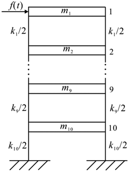
A 10-storey shear frame.

Identified results of one calculation in the case of 5% noise level and three response points: (a) convergence of identified
In this article, the damage is simulated by reducing the stiffness value of the structure, and it is assumed that the structure has suffered 30% damage at
In this article, Newmark method 28 is used to calculate the structural response. The time-sampling interval is 0.01 s, and the total calculation time is 10 s. Noise is added to the response of degrees of freedom chosen as the response points by the following equation

in which
Algorithm validation
First, the load and unknown parameters are identified without considering the effect of noise. The initial values of the stiffness are all assumed to be 1000 Nm−1 and the initial values of
Identified results of the load and unknown parameters with no noise in the response.

RP: response points; TR: truncation ratio; IV: identified value.
As Table 1 shows, in the case of only two response points, the load and unknown parameters can be accurately identified, which verifies the correctness of the algorithm proposed in this article.
Effect of noise level and number of response points on the identified results
Although accurate identified results of the load and unknown parameters can be obtained without considering the effect of noise, the response always contains the noise components, and the existence of noise greatly amplifies the effect of the ill-conditioning of the inverse problem on the identified results. In this section, noise with different levels is added to the response to simulate the measured response, and different numbers of response points are taken to identify the load and unknown parameters to further verify the applicability of the proposed algorithm.
In addition, it should be noted that because the response contains random noise, even if the same level of noise is added to the response, the final identified results are certainly not the same, especially for unknown parameters. In this article, noise with the same level but with different distributions is added to the response, and multiple sets of identified results of the load and unknown parameters are obtained by multiple calculations. Finally, the mean values and standard deviations of the identified values of the unknown parameters are calculated. Because the mean value of an identified parameter is not necessarily equal to its actual value, the error of the ith unknown parameter is defined by the following equation

in which
The load identified error is determined by the average error of the multiple sets of the identified load. The results obtained in this way can better reflect the accuracy and stability of the algorithm.
The truncation ratio and initial values of the unknown parameters are the same as those in the preceding section. Table 2 shows the mean values and errors of the identified unknown parameters and the errors of the identified load in the case of different noise levels and different number of response points. The convergences of the unknown parameters and the comparison of the identified
Identified results of the load and unknown parameters with different levels of noise and different number of response points.

RP: response points; NL: noise level; MV: mean value.
In summary, satisfactory identified results of the load and unknown parameters are obtained in all cases in Table 2, especially the structural stiffness. Even in the case of 10% noise levels, the errors of the identified stiffness are not greater than 1.7% when only two response points are used, which is completely acceptable in engineering.
Furthermore, as the noise level increases, the errors of the identified results increase, and by increasing the number of response points, the errors decrease significantly. Therefore, when more accurate identified results are necessary, more response points must be selected, especially when the response is seriously polluted by noise. In addition, the convergences of unknown parameters have obvious convergence points as shown in Figure 2(a)–(e); thus, there is no requirement for a convergence condition for the proposed algorithm.
Effect of truncation ratio on the identified results
A parameter called the truncation ratio is defined in this article; thus, this section studies its effect on the identified results.
To compare the effect of the truncation ratio on the identified results more directly and effectively, in the case of 5% noise level and three response points (1, 3, and 5 degrees of freedom), multiple sets of responses with the same noise level, but the noise is different in the time history, are generated first. Next, the multiple generated sets of responses are used to identify the load and unknown parameters under the different truncation ratios from 0% to 10%. Finally, the mean values and errors of the identified results are obtained at different truncation ratios. The initial values of the unknown parameters are the same as those in the preceding section. The curves of mean values and errors of the identified results of the stiffness in the case of different truncation ratios are shown in Figure 3.

Identified results of stiffness with different truncation ratios: (a) mean value and (b) error.
As Figure 3 shows, when the truncation ratio is 0%, that is, when the positive and negative properties of the perturbation terms of the unknown parameter are determined in the case where the sequence
Therefore, a conclusion can be drawn that the introduction of the truncation ratio effectively reduces the error and increases the stability of the proposed algorithm. In addition, in a very large range of the truncation ratio, the identified value can approach the actual value, illustrating that the truncation ratio is not a difficult parameter to determine.
Effect of initial values and norm types on the identified results
To study the effect of initial values of unknown parameters on the identified results, with different initial values of the stiffness, the convergences of

Convergences of identified
As Figure 4 shows, with different initial values and different norm types, the final identified values of
A simply supported beam
A simply supported beam with a uniform cross-section is used as the research model in this section, as shown in Figure 5. The transverse vibration equation of a beam under a concentrated load is as follows

in which

A simply supported beam.
With the basic idea of the reference,
29

Using the orthogonality of the mass, damping, and stiffness with respect to the structural modal shapes, one can obtain

in which
Substituting equation (23) into the expression of the modal load in equation (24), one can obtain

The dynamic response of the simply supported beam can also be obtained using Duhamel integral together with the modal superposition method

in which
Suppose that
in which
The above equation can be simplified as

Thus, the same form as equation (2) is obtained, and the load and structural unknown parameters can be identified simultaneously by the algorithm proposed in the preceding section.
In this article, the cross-section of the beam is rectangular; the beam height, width, and length are 0.005, 0.06, and 2 m, respectively; the elastic modulus E is 1.8e11 Nm−2; the density

Identified results of one calculation in the case of set 4: (a) convergence of identified E, (b) convergence of identified c, (c) convergence of identified
The elastic modulus E, damping c, and load position
To study the effect of the distribution of the response points on the identified results, six sets of response points are selected, and the identified results of the load and unknown parameters with different sets of response points are shown in Table 3. The convergences of the unknown parameters and the comparison of the identified
Identified results of the load and unknown parameters with different sets of response points.

RP: response points; MV: mean value.
As Table 3 shows, the more concentrated the distribution of response points, the larger the errors, even though the response points are distributed in the vicinity of the midpoint of the beam, where the response is relatively large. This is because the response history of one point is too much like the others under these circumstances, which leads to a reduction in the information about the load and structural parameters contained in the response. When two of the four response points approach the two endpoints of the beam, the errors are slightly larger. Therefore, it is also not recommended for the response points to be distributed near the two endpoints of the beam because the response of this part of the beam is much smaller.
Conclusion
This article proposes a new algorithm for the simultaneous identification of the load and unknown parameters of the structure using only a few response points based on the perturbation method. The algorithm only requires initial values for the unknown parameters, which are not required for the loads. In addition, the proposed algorithm does not require a convergence condition for the iteration process. In addition, the regularization parameter does not need to be calculated in each iteration step, thereby effectively increasing the efficiency of the algorithm. Furthermore, a parameter called the truncation ratio is defined, and the identified results for an example show that the introduction of this parameter greatly reduces the errors obtained with the proposed algorithm and that the best range of this parameter is relatively large. In a case with different noise levels and different numbers of response points, satisfactory results are all obtained, illustrating that the algorithm provides good accuracy and applicability. Moreover, the proposed algorithm is also applied to the identification of a simply supported beam, and the study of the distribution of response points shows that when the response points are distributed over the full beam, the identified results are better than that when the response points are distributed over only part of the beam.
Footnotes
Handling Editor: Crinela Pislaru
Declaration of conflicting interests
The author(s) declared no potential conflicts of interest with respect to the research, authorship, and/or publication of this article.
Funding
The author(s) disclosed receipt of the following financial support for the research, authorship, and/or publication of this article: This research was supported by the National Natural Science Foundation of China (grant no. 51579084), the Jiangsu Province Key R&D Project (grant no. BE2017167), and the Fundamental Research Funds for the Central Universities (grant nos. 2018B48514 and 2018B685X14).