Laser simulator

Abstract

A novel technique called laser simulator approach for visibility search graph-based path planning has been developed in this article to determine the optimum collision-free path in unknown environment. With such approach, it is possible to apply constraints on the mobile robot trajectory while navigating in complex terrains such as in factories and road environments, as the first work of its kind. The main advantage of this approach is the ability to be used for both global/local path planning in the presence of constraints and obstacles in unknown environments. The principle of the laser simulator approach with all possibilities and cases that could emerge during path planning is explained to determine the path from initial to destination positions in a two-dimensional map. In addition, a comparative study on the laser simulator approach, A* algorithm, Voronoi diagram with fast marching and PointBug algorithms was performed to show the benefits and drawbacks of the proposed approach. A case study on the utilization of the laser simulator in both global and local path planning has been applied in a road roundabout setting which is regarded as a complex environment for robot path planning. In global path planning, the path is generated within a grid map of the roundabout environment to select the path according to the respective road rules. It is also used to recognize the real roundabout from a sequence of images during local path planning in the real-world system. Results show that the performance of the proposed laser simulator approach in both global and local environments is achieved with low computational and path costs, in which the optimum path from the selected start position to the goal point is tracked accordingly in the presence of the obstacles.

Introduction

Path planning in robotic research is one of the most complicated problems that can occur during autonomous navigation in unknown environments. In path planning approaches, the path trajectory is planned continuously between the start and goal positions while attempting to avoid colliding with obstacles and other objects within the path. Two kinds of path planning approaches for mobile robot have been established, namely the global and local path planning. In the former, the surroundings of the environments are totally known and the collision-free trajectory is usually accomplished off-line whereas in the latter, the surroundings of the environments are unknown and feedbacks from sensors are required for real-time path planning. ¹

In general, the process of path planning involves three main tasks: (i) sketch clearly and informatively the robot’s terrain, (ii) determine the collision-free path from start to target points and (iii) seek for optimum path to reach the goal. ²

The current path planning methods have been utilized widely to find the shortest path, optimum path to determine the goal, collision avoidance and collision-free path navigation in difficult environments.

However, none of these approaches can be used effectively in constrained environments such as the road and factory settings, where there are some rules and constraints that must be strictly adhered. Owing to the constraints, current classical path planning algorithms are no longer suitable for path determination in the maps of the constrained environment. In addition, the generated path has to guarantee low computational and path costs, avoid obstacles and follow a smooth path to reach the goal.

Related works

Many approaches have been developed to accomplish the path planning tasks in both global and local environment settings.

In global path planning, a family of heuristic search algorithms depending on A* and D* algorithms has been widely used in robotic applications to determine the optimum path from a given starting node to predefined destination position. In general, these approaches comprise two kinds of cost functions. The first is the movement cost which is used to evaluate the moving of particle from the initial cell to each cell on the grid map. The other function is the goal cost which is used to estimate the movement from each cell on the space grid to target cell while avoiding the obstacles.

Lifelong planning A* ³ and D*-Lite ⁴ algorithms by the same authors were proposed to solve the shortcomings and problems of A* and D* methods, particularly when the edge weights are changed, no edges to be detected in the path and the cost function has an infinite value. In general, those algorithms can plan for the shortest path without looking at the robot kinematic and dynamic constraints. A new feasible edge with combined AD*algorithm applied in the robot workspace has been introduced by Kushleyev and Likhachev ⁵ to meet the robot’s kinematic and environments dimensions and find the optimal path. All these algorithms are in fact a search-based algorithm in which they must know the environment cells well before generating the path. This searching task is leading to higher computational cost that is required to calculate the distance to reach all cells of the grid and choose the suitable one for the path. The main concerns of these algorithms are to find the shortest path between the start to goal positions; however, there are no considerations for the constraints and rules in the environment.

The artificial intelligence (AI) methods are commonly used to determine the robot path due to their learning capabilities and ability to deal with non-linearity mapping such as fuzzy logic, neural network, genetic algorithm, ant colony and particle swarm optimization. The main drawbacks of AI-based path planning is the limitation of robot features that has to be taken into consideration when generating path planning. Increasing the number of features will lead to an increase in the complexity of the algorithm.

Singh et al. have proposed a neural network algorithm for robot navigation in unknown environments with static and dynamic obstacles.

The input of this system has four layers; three layers for estimating the obstacle distance (right, left and front) and one layer for determining the angle between the robot and the goal position. The output layer is the heading angle of the robot. ⁶ The system mainly focuses on avoiding the obstacles in unknown environments.

With fuzzy logic algorithm, a mobile robot navigation in traversability of roughness terrain in a disaster environment has been accomplished. ⁷ A real-time mapping was built based on signals of laser range finder (LRF) and the traversability analysis is performed based on a fuzzy logic approach.

The fuzzy inference engine involves two input membership functions, namely the terrain roughness and slope. The output membership function is a terrain traversability which was then inserted to a vector field histogram (VFH) to calculate the position and velocity of robot. The fuzzy system focused only on the roughness and slope of the terrain and no others factors were taken into consideration such as obstacles, borders and so on.

A genetic algorithm has been used for a wheeled mobile robot (WMR) navigation in static, dynamic and unknown environments. ⁸ The genetic algorithm enabled the robot to avoid the obstacles well in an unstructured environment. This algorithm is able to determine the feasible path in acute shaped obstacles such as (U) or (V), find the shortest path and reduce the goal search time. In general, this work is just concerned on acute dynamic obstacles and shortest path determination. A multi-objective feasible path planning is determined by ant colony algorithm for obstacle avoidance. ⁹ The ant colony algorithm is combined with point-to-point sampling approach to estimate the position of obstacles. The proposed algorithm performed better than other point-to-point sampling approaches in terms of path quality and speed.

A reinforcement learning (RL) algorithm has been used for balancing a lower body of humanoid robot (NAO HR) during standing up, sitting down, running and walking operations. ¹⁰ The three-dimensional (3D) RL trajectory is converted into reference position of the robot joints using inverse kinematic, which helps to minimize the dimensionality of the learning process. The results of simulation show that the lower body of HR is stabilized well at upright position when the RL cost function is maximized. An enhancement to the RL method is provided by a central pattern generator algorithm to balance the 3-links lower body HR robot, which has significantly reduced the dimensionality of the learning problem. ¹¹

The AI-based path planning is taking only some features into consideration, namely the shortest path, obstacle avoidance and global–local path planning. By adding additional features, it will increase the complexity of the algorithm and computational cost of these algorithms. To include constraints in such algorithms, we need to generate more features to these algorithms, thereby increasing the computational cost.

With roadmap path planning method, the initial point is matched to the goal by arc or straight lines. The space graph nodes are the initial, goal points and obstacles vertices.

The nodes that are seemingly visible to each other are connected by a series of lines. The main methods for road mapping are the visibility-based search graph and Voronoi-based diagram. In the visibility search graph, the cost of each line from the start to goal nodes is accordingly calculated and the algorithm selects the optimum trajectory to the goal that does not collide with the obstacles. Meanwhile, in the Voronoi diagram with fast marching (VDFM), the path is comprised of a number of points that are equidistant from the surrounding polygons or obstacles which are connected together to form the Voronoi’s edges. ¹² Santiago et al. has introduced a hybrid method employing the use of VDFM to find a global path of robot in a map. In this method, the VDFM is applied firstly to extract the safest path in the environment and secondly, fast marching is implemented to find the best path between the start and goal positions using the speed function which does not change its sign while moving to the goal. ¹³ Although the road map approach needs low computational cost, its path cost becomes high due to its arbitrary connection with the environment vertices, which in turn makes the path always longer compared to other methods.

A probabilistic path planning method, the so called rapidly exploring random tree (RRT) has been developed by LaValle and Kuffner to find the path in a configuration space. ¹⁴ In this method, a group of trees are grown from the start C-space to explore all cells in the configuration space while taking a random sample of C space in each step. It starts to explore from the tree’s nearest vertex by adding a new edge point to the sample. This vertex expands later by adding a Voronoi bias to the configuration space. As the boundary vertex of the tree has the biggest Voronoi region, it will be selected for path expansion. To solve the problem of producing several branches in randomized trees, potentially created in the path, a new heuristic technique that is integrated into the RRT (He-AT-RRT) algorithm has been introduced to give the capability of the RRT algorithm to select the randomized point in the explored space that are located close to the goal. ¹⁵

A new version of RRT algorithm family, the so called RRT^X is used in dynamic environments with moving and unexpected obstacles. ¹⁶ In contrast with other single query RRT algorithms, this algorithm tries to update the search graph over the time based on the new locations of the obstacles without any priori off-line computations. The algorithm remodels the existing search graph once the obstacles are found by switching from the shortest path process to goal sub-tree, rewiring and cascading processes. The main drawbacks of the RRT family algorithms are: (1) high computational time needed due to the necessity to explore the whole map, (2) could not deal with the constrained environment since the replanning path concept in these methods is always associated with the obstacles avoidance without any considerations to the constraints during the movements, (3) creates a non-smooth path due to the continuous repairing of the path and (4) usually, it could not guarantee to reach to the goal through an optimum path.

In the local methods-based path planning, a path determination method based on the guidance through the artificial potential field (APF) approach and stochastic researchable set (APF-SR) has been used for static and dynamic obstacles avoidance. ¹⁷ The sampling-based stochastic method is used to find the collision-free path in static environments and APF is used to avoid the moving obstacle in its path. The proposed method has low computational cost in comparison with other sampling-based methods and can generate a flexible path while navigating in crowded environments with 300 obstacles. However, it still needs to explore the whole environment to determine the optimum path which results in higher computational cost.

A navigation system using a VFH method and global positioning system (GPS) has been used to enable a self-driving car to reach the destination position with a safe path and obstacle avoidance in real-world environments. ¹⁸ It incorporates a VFH as local planner with GPS as a global planner with a proportional–integral–derivative controller to autonomously navigate in restricted environments. The VFH method has been implemented with two different Light Detection and Ranging (LIDAR) to build a 3D Cartesian coordinate map, which helps to overcome the conventional LIDAR system in terms of accuracy, reliability and efficiency. No constraints are involved in the path of this vehicle. Similar to APF, all cells in the map have to be checked to find the suitable path between the start to goal positions.

Nearness Diagram Approach is used for path planning of mobile robots to avoid obstacles when moving in a complex terrain. The configuration space of robot is separated into sub-sectors that are centred in the mobile robot location with several bisector angles. ¹⁹ A suitable distance between the mobile robot and the obstacles is required to guarantee the safety of driving in the whole space. Two functions are estimated in this approach; the nearness distances from the robot centre position which represent the approaching of the centre of robot to obstacles and the nearness distances from the mobile robot boundaries which represent the approaching of the robot bounds to obstacles. It has a high computational cost due the need to explore the whole map to generate the right heading angles for movement.

Bug algorithm family is well known for obstacle detection-based local path planning with less data acquired from the range sensors. ²⁰ As a result, the path is determined by matching the current position with the edge of the nearest obstacle. Several types of bug algorithms are typically used with sensors to find the shortest path from start to goal positions such as VisBug, DistBug, TangentBug and PointBug (PB). In the PB algorithm, three points are used to generate the robot’s path, namely the current sudden point, sudden point on the obstacle edge and previous sudden point. A logical triangle is then formed between these three points to generate the path. The PB algorithm shall be used in the comparative study with the proposed laser simulator (LS) approach.

The LS approach has been initially introduced by Ali et al. to find the optimal path in restricted environments with the presence of multiple constraints during the robot motion in the roads and factories environment. ^{21 –23} The main feature of the LS approach is the capability to deal with the environmental constraints and unknown environments, both in global or local path planning. More details about this method will be explained in the third section.

Table 1 shows a comparison between the previous approaches. This comparison has been accomplished based on the following criteria: (1) Two-dimensional (2D) maps with polygons borders are considered for global path planning. (2) Small-scale environments (1–10 m) are considered in the local path planning. (3) The capability of the algorithm to avoid obstacles (moving or static) is considered, no matter whether the size of obstacles is big or small. (4) The appearance of the path can help to estimate the path cost, smoothness and constraints. (5) The computational time is considered always high for the search-based algorithms and low for the selected-based algorithms.

Table 1.

Comparison between path planning approaches.

Method	Global path	Local path	Dynamic obstacle	Static obstacle	Computational time	Path smoothness	Path cost	Constraints
A*A family	Yes	No	No	Yes	High	Yes	Low	No
AI family	Yes	Yes	Yes	Yes	High	No	Medium	No
RRT family	Yes	Yes	Yes	Yes	High	No	High	No
RM family	Yes	Yes	Yes	Yes	Medium	No	Medium	No
APF family	Yes	Yes	Yes	Yes	High	No	Medium	No
VFH	No	Yes	Yes	Yes	High	Yes	High	No
NDS	No	Yes	Yes	Yes	High	Yes	High	No
Bug family	No	Yes	Yes	Yes	Low	No	Low	No
LS	Yes	Yes	Yes	Yes	Low	No	Low	Yes

AI: artificial intelligence; LS: laser simulator; A*A: A* Algorithm; RRT: rapidly exploring random tree; APF: artificial potential field; VFH: vector field histogram; RM: road mapping; NDS: nearness diagram approach.

As shown in Table 1, the previous path planning methods have been utilized to find the shortest path, optimum path to determine the goal, collision avoidance and collision-free path navigation in difficult environments. However, none of these approaches can be used effectively in constrained environments such as the road and factory settings. In such areas, there are rules and constraints that must be strictly adhered. Owing to such restrictions and limitations, most of the above-mentioned path planning approaches are no longer suitable in determining the optimum path for robotic navigation in restricted environments. ^{19 –21}

This article presents a novel path planning approach, the so called LS in a complete form to find the optimum path in restricted environments with the presence of multiple constraints in the robot motion. It is in fact emulating a LRF device.

The features of LS approach have been compared with the well-known approaches such as A* algorithm (A*A), VDFM and PB algorithms. A case study on the implementation of the LS technique for global and local path planning of a WMR in a road roundabout setting is accomplished to search for the optimum path between the initial and target positions while avoiding obstacle. The roundabout has a circular area and the WMR must travel within the circular path to find the exit branch without any reference to the traffic light signal unlike the cross intersection junction in which the vehicle has to rely on the traffic light signal and rules when choosing the exit branch.

Such environment has been considered a relatively dangerous area for robot path planning since the WMR has to follow the constraints in its path such as true branch detection, rotation on the roundabout before taking the exit and going always to the right or left sides depending on the common driving practices (and rules) of some countries. ²² Furthermore, to date, no comprehensive study has yet been done to model and generate a complete real-time navigation in a roundabout setting. ²⁴

LS principle

A new approach has been introduced in this article to search for the optimum path in unknown and restricted terrains while avoiding obstacles. It is emulating the LRF when it is used to detect the robot environment boundaries and build a polygonal map. In this LS approach, it is possible to apply constraints on the robot trajectory while navigating in complex terrains such as factories and road environments. The main advantage of this approach is its ability to be used for both global and local path planning with the presence of obstacles in unknown environments.

The principle of LS is described according to the following steps:

i. The surroundings of the environments shall be represented as 2D grid maps f(x, y) as shown in Figures 1 and 2. The environmental boundaries and obstacles are projected as polygonal lines such as arc, circular, tangential and straight lines on the map. The obstacles can be static or dynamic objects that might exist during navigation.

The initial point (x _int, y _int) and destination point (x _g, y _g) are well known before the starting of path determination.

The LS is imitating a LRF device where it generates several series of points in front of the robot starting from first cell of the map in front of the current position to the left and right directions as vertical or horizontal lines, which are always perpendicular to the robot motion trajectory as shown in Figure 2, assuming that the starting robot position is (x _int, y _int).

When there are more than one possible ways to arrive at the destination, the collision-free path can be determined using cost function as in equation (1)

$T=f(G(x,y)+\text{CR}(x,y))$

1

where T is the cost function to reach the goal, G(x, y) is a function that measures the distance between the current position and the destination while CR(x, y) is a function that describes the rules and constraints to be adhered with. If there are multiple choices that LS can pass through, LS will evaluate all paths. This evaluation can be presented in the form of maximum or minimum distances from each chosen location to reach the goals, for example, in the corridor environment as shown in Figure 3, the right door for LS path is the nearest to goal, however in a roundabout as shown in Figure 7, the right outlet branch is deemed the farthermost. The constraints function CR(x, y) is represented in a 2D map when there is a gradual change from a series of horizontal lines to vertical lines or vice versa as shown in Figures 1 and 3 to 7. The switching from vertical to horizontal lines can be detected if the next line becomes suddenly longer than the previous line on one side or both sides. This means that the constraint occurs on the right or left sides from the current position if the next line becomes longer than the previous line by certain thresholds as illustrated in the following conditions

$\text{CR}=\left\{\begin{array}{c}\text{CR}\_\text{right side} \text{if} L_{n+1}-L_n>h_{\text{R}}\\ \text{CR}\_\text{left side} \text{if} L_{n+1}-L_n>h_{\text{L}} \\ \text{CR}\_\text{both sides} \text{if} L_{n+1}-L_n>h_{\text{R}} \text{and} L_{n+1}-L_n>h_{\text{L}}\end{array}\right\}$

where L_n is the length of the current line, L_{n +1} is the length of the next line, h _R is threshold on the right side (h _R > 50% of L_n ) and h _L is threshold on the left side (h _L > 50% of L_n ).

Figure 1.

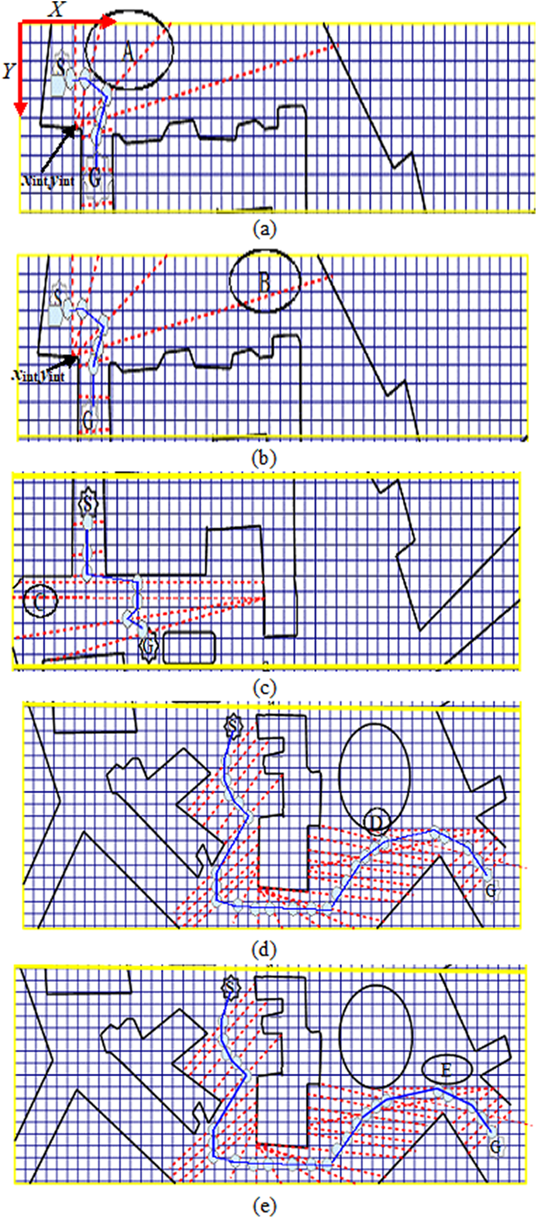
LS approach (red colour) applied on 2D environment (polygons with black colour) to find the collision-free path (blue colour): (a) Case A – a single border detected only; (b) case B – a single border detection with long tangential line; (c) case C – shift from small to large regions; (d) case D – detection of obstacles; and (e) case E – selection of shortest path to destination. LS: laser simulator; 2D: two-dimensional.

Figure 2.

LS algorithm producing a series of points representing: (a) horizontal lines; (b) vertical lines; point () is the candidate of the path; point (•) is the previous lines path candidate. LS: laser simulator.

Figure 3.

Comparison between LS, A* Algorithm and VDFM: (a) Clear border environment with paths generated by LS (green) and A*A (purple); (b) clear border environment with paths generated by LS (green), A*A (purple) and VDFM (red); (c) noisy environment with paths generated by LS (green) and A*A (purple); (d) noisy environment with paths generated by LS (green), A*A (purple) and VDFM (red). LS: laser simulator; A*A: A* Algorithm; VDFM: Voronoi diagram with fast marching.

Figure 4.

Computational costs for the LS, A*A and VDFM: (a) Computational cost for clear environment and (b) computational cost for noisy environment. LS: laser simulator; A*A: A* Algorithm; VDFM: Voronoi diagram with fast marching.

Figure 5.

Path costs for the LS, A*A and VDFM with fast marching approaches: (a) Path cost for clear environment and (b) path cost for noisy environment. LS: laser simulator; A*A: A* Algorithm; VDFM: Voronoi diagram with fast marching.

Figure 6.

Constraints of the LS path in 2D environments; the notations 1 to 4 represent the constraints of movement; point () is the starting position and point () is the goal position. LS: laser simulator; 2D: two-dimensional.

Figure 7.

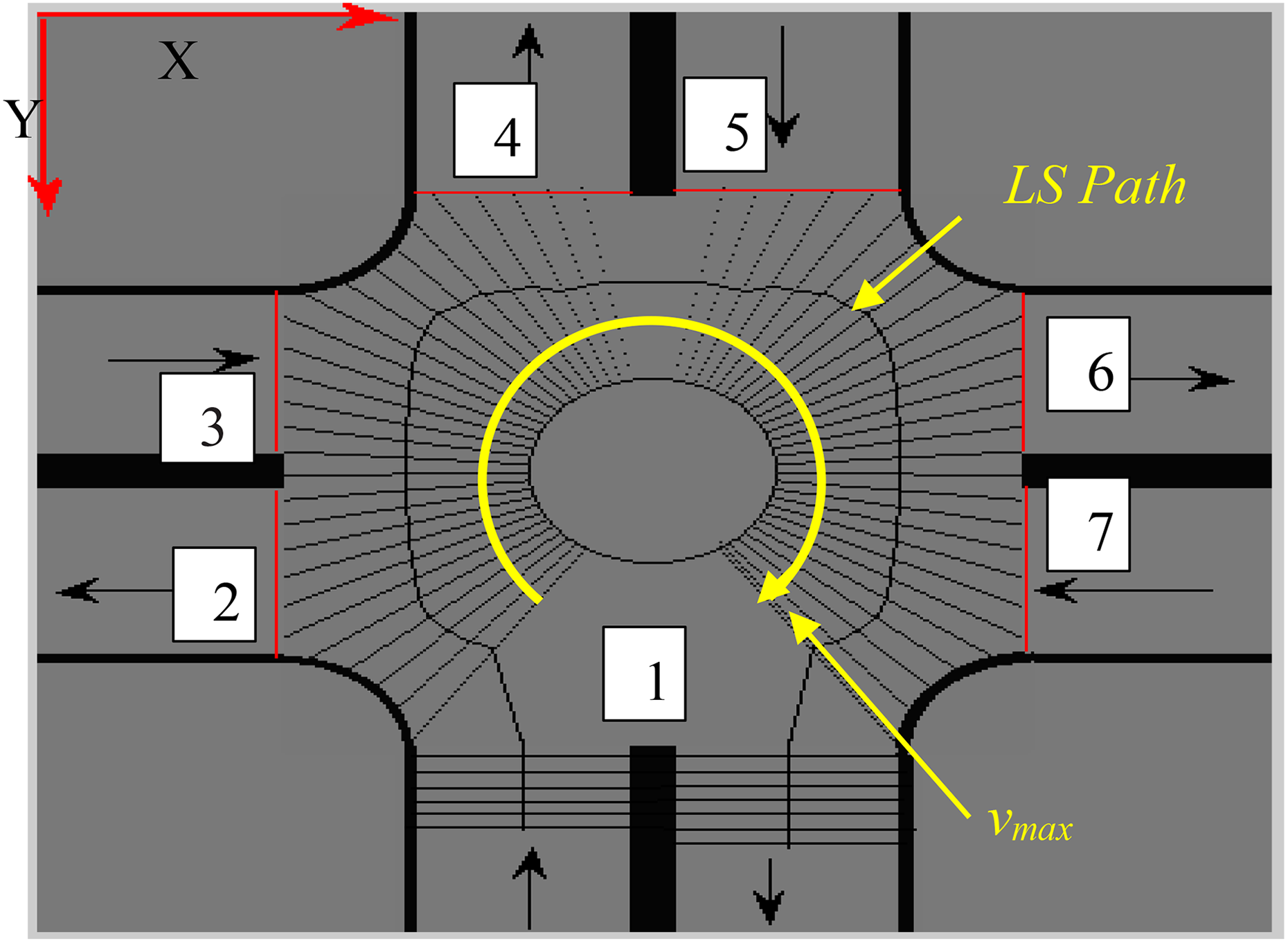
Roundabout settings with LS path; the notations 1 to 7 represent the constraints of movement; ν _max is the maximum rotational angle of last line in LS. LS: laser simulator.

The algorithm will then evaluate all the constraints and choose to go with the one that is nearest to the goal. More details on how to generate the constraints are illustrated in the fourth section.

The shortest path between the start to goal positions is always selected in case if there are no constraints as shown in Figure 1 (case E).

v. When an obstacle is detected, its border is considered as one edge of the generated lines and LS lines will be generated between the obstacle edges and other borders as shown in Figure 1 (case D). Equations (2 –7) are applied to find the path in this case.

As mentioned in point (iii), the LS is imitating the LRF to detect the borders of the 2D grid map environments, which is accomplished by generating vertical or horizontal series of points as lines to detect the borders of the environments. In the case of vertical series of points as vertical line as shown in Figure 2, if the robot is located at the initial position (x _int, y _int), a series of points representing a vertical line will be created through the LS in front of the robot starting from first cell of the map in front of the current position (x _c, y _c) to the left and right direction until it touches the border as defined in equations (2) and (3). The points (x _int, y _int) and (x _c, y _c) are equally positioned in y direction and x _c is assigned to be bigger than x _int by 1 cell.

On the right side of point (x _c, y _c), the points can be generated using equation (2)

$y=y_{\text{c}}+i_1$

2

On the left side of point (x _c, y _c), another set of points is generated using equation (3)

$y=y_{\text{c}}-i_2$

3

where i ₁ = 1: R and i ₂ = 1: L are the count of cells in the grid map from the right and left of the current position (x _c, y _c), respectively, until the generated points hit the borders on the right (R) and left (L) sides of the environment. The size of the cells isn’t constant and depends on the resolution of map’s image.

The x position for the first line remains constant and equals to x _c, which is the first cell of the map in front of the current position (x _c, y _c).

The candidate point (x _p1, y _p1) for the path in this first vertical line has the following dimension as defined in equation (4)

$\begin{array}{l}{x}_{\text{p}1}=x_{\text{c}}\\ y_{\text{p}1}=y_{\text{c}}+\frac{i_2-i_1}{2}\end{array}$

4

The x position of the candidate point (x _p2, y _p2) for the second line can be determined by equation (5) for forward direction movement

$x_{\text{p}2}=x_{\text{c}}+f_1$

5

For backward direction, the equation can be written as in equation (6)

$x_{\text{p}2}=x_{\text{c}}-f_2$

6

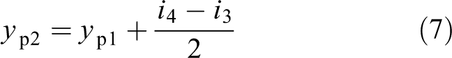
where f ₁ and f ₂ are the incremental cells in x position, it should be assigned with small value to enhance the accuracy of the trajectory. By repeating equations (2) and (3) to count the number of cells on the left and right of point (x _p2, y _p1), the y position of the candidate point (x _p2, y _p2) is expressed as in equation (7)

$y_{\text{p}2}=y_{\text{p}1}+\frac{i_4-i_3}{2}$

7

where i ₃ = 1: R and i ₄ = 1: L are the count of cells in the grid map from the right and left of the current point (x _p2, y _p1), respectively, until the generated points hit the borders on the right (R) and left (L) sides of the environment.

By the same way, we can determine the other vertical lines of LS. Similarly, we can use the same equations (1 –6) to determine the horizontal series of points as horizontal line, by just swapping the x and y directions. The candidate point (x _p1, y _p1) for the path in this first horizontal line has the following dimension as in equation (8)

$\begin{array}{l}{y}_{\text{p}1}=y_{\text{c}}\\ x_{\text{p}1}=x_{\text{c}}+\frac{i_2-i_1}{2}\end{array}$

8

The second candidate points can be determined using equation (9)

$\begin{array}{l}{y}_{\text{p}2}=y+f_1\\ x_{\text{p}2}=x_{\text{p}1}+\frac{i_4-i_3}{2}\end{array}$

9

where i ₁, i ₂, i ₃ and i ₄ can be defined in the same way as in equations (2 –6) but in the x direction. f ₁ and f ₂ are also similar to equations (5) and (6) but in the y direction.

Three main cases can be observed in the collision-free path of the robot as follows:

Two-side–borders detection

The LS algorithm generates a series of points from the first cell of the map located in front of the current position to the left and right directions to represent vertical and horizontal lines based on the related equations as shown in Figure 2

The LS approach selects a single point among the series of generated points as the proposed candidate for the path as depicted in Figures 1 and 2 (located roughly in the middle of lines). A particular case is said to have occurred when the path shifts from a small region to a large region or vice versa as shown in Figure 1 that is represented in case C. To prevent getting a drift in such a case, a set of new lines with in-between distance shall be deliberately generated.

The start and end points of each generated line on the left and right sides of the horizontal lines can be described as in equations (8) and (9).

One-side–border detection

For only one border that can be detected by the series of points, the LS algorithm will in turn generate a series of tangential lines that converge at a single point already determined as shown in Figure 1 (case A). The tangential lines are in fact produced from a point on the existing border and rotated at a certain angle until the other border is detected as shown in Figure 1 (cases A and B). The distances between the proposed candidate points of the tangential lines and the existing border’s points (x _int, y _int) remain constant. The rotational lines are described as in equation (10)

$x=\left(y-y_{\text{int}}\right)\text{tan}\left(\epsilon \right)+x_{\text{int}}$

10

where x _int and y _int are the points’ coordinate system when the LS algorithm starts the rotation as shown in Figure 1. ε is a slope of the tangential line against the vertical ones. Another case is noticed when the new tangential line intersects with the other border at a relatively long distance in comparison to the previous tangential line as shown in Figure 1 (case B). In this state, the displacement between the existing border and proposed candidate points remained similar to the previous tangential line.

None of the borders are detected

In this case, the LS algorithm generates tangential lines starting from the current cells till it finds one or two borders. Equation (10) is used for generating such lines.

Comparing LS algorithm with other approaches

A*A algorithm was first chosen to benchmark the LS algorithm, since it is well known and commonly used method for global path planning as shown in Figure 3(a) and (c). The LS was also compared with the VDFM technique ¹⁰ as shown in Figure 3(b) and (d), notably depicted with netlike formation. The comparison is performed using a 2D environment map with clear border (Figure 3(a) and (b)) and noisy environments (Figure 3(c) and (d)).

Three parameters have been considered for the comparison, namely the computational cost, trajectory cost and path smoothness. The trajectory cost is defined as the complete distance required to reach the goal position from the starting point. As it is preferred to reach the goal with a shortest possible time during path planning, a computational time is regarded as the main feature for path determination approach and is known as the time spent to reach the destination from the initial position. The path smoothness is recognized through the trajectory patterns of the generated paths by different approaches.

The computational cost of the LS is usually smaller than the time executed by the A*A and VDFM to reach the goal from the starting position as shown in Figure 4. In the clear boundary environment as depicted in Figure 3(a) and (b), there is a huge difference in the computational time between the LS, A*A classic algorithm and VDFM approaches.

However, the differences become smaller in noisy environments as shown in Figure 3(b) and (d). The computational costs for all approaches with 20 trials and considering clear and noisy environments are presented in Figure 4. The mean values of the computational costs for clear environment in Figure 4(a) are 91.65 s, 174.25 s and 100.6 s for LS, A*A and VDFM algorithms, respectively. In contrast, these values for noisy environment as depicted in Figure 4(b) are found to be 208.3 s, 384.65 s and 238.7 s, respectively, implying small differences.

The path costs for all approaches considering clear and noisy environments with 20 trials are illustrated in Figure 5. The path costs for the LS and A*A approaches are approximately similar.

However, there is a noticeable difference between the LS and VDFM algorithms. Meanwhile, the difference is slightly smaller between the A*A and LS algorithms as shown in Figure 5 which may be due to the fact that the A*A algorithm does not follow the rules and constraints in its movement. In addition, the robot terrain is regarded as an unknown environment for LS, while it is already known for A*A. On the other hand, the VDFM algorithms have the highest path cost because the coordinate system of the cells’ centres in VDFM is changing arbitrarily in x and y direction which in turn causes the algorithm to oscillate and fluctuate while moving towards the goal.

The mean values of the path costs for clear environment presented in Figure 5(a) are 189.85 mm, 181.25 mm and 300.05 mm for LS, A*A and VDFM, respectively. However, for noisy environment as shown in Figure 5(b), these values are 399.65 mm, 331.95 mm, and 566.45 mm, respectively. From Figures 4(b) and 5(b), it seems that the differences of the computational and path costs between LS, A*A and VDFM in the noisy environment become smaller in some trials. This is due to that the noises are acting as excitation signals and lead to an optimal solution. ²⁵ However, the cost values are almost similar in all trials for clear environment as shown in Figures 4(a) and 5(a).

The constraints to reach the goal from start position in the environment as shown in Figure 6 is to go straight through the corridor until it finds the right door of the goal’s room. The doors are discovered if the next vertical line becomes longer than previous line on one side. We have four doors that the LS path will pass through them. Doors 1 and 2 have positions that will make the distance to the goal becomes longer than any candidate points of the path (middle of vertical lines), and hence they will be excluded. Doors 3 and 4 are of potential values for the LS path and since LS does not know the environment yet, it will first test whether there are other doors after Door 3, so that it will generate vertical lines until it reaches Door 4. Now, it will choose Door 4 as the LS path and draw the testing lines as real lines. Doors 1, 2 and 3 are considered as the environment borders after LS confirms that they are not of potential value for the path.

For the path smoothness feature as shown in Figure 3, it is noticed that the path pattern of A*A shows a little bit smoother than LS, but the VDFM method produces the worst trajectory. This is because the LS lines are generating only as vertical and horizontal lines in the polygon maps which can be improved if the LS is generating lines in all directions. In comparison with the VDFM, LS exhibits smooth trend unlike the one shown by the VDFM cells behaviours.

As featured in Figure 6, the constraints 1 to 4 are represented in a 2D map when there is a change of vertical lines to horizontal lines. After evaluation of all the constraints, the algorithm choose to go with the fourth one.

Implementation of LS for path planning in a road roundabout environment: A case study

The LS approach is implemented to find the collision-free path within the road roundabout, which is considered as complicated terrains involving constrains such as bends, intersections and priority rules. Consequently, it is required to develop an algorithm with the capability to make decision for selecting the optimum trajectory from the entrance to exit of the roundabout. LS algorithm has been implemented in a roundabout terrain in two ways, namely the global path planning in the grid maps and local path planning in the real road roundabout environments. This is duly described in the respective subsections as follows:

Part A: Global path planning in the grid map

It is used to enable a specific point to move from start to goal positions in a roundabout environment.

The main features of the road roundabout environment have been modelled in this simulation, namely border sides or curbs, middle road borders and the intersection of roundabout. As has been previously mentioned, a 2D grid map is utilized to represent the road roundabout setting in MATLAB using an image processing toolbox in which a pixel represents one cell of the 2D grid map. The roundabout environment is modelled as a circular arc located in the middle of the roundabout as shown in Figure 7. The LS generates a series of points as horizontal/vertical lines to locate the road’s curbs, where the roundabout is not found yet.

When negotiating a bend (turning), it will generate another series of points as tangential lines as shown in Figure 7 while at the same time, applying an image processing algorithm to detect the intersection of edges.

The roundabout settings are classified into three main regions, namely the entrance, exit and centre regions.

As shown in Figure 7, there are seven constraints (1–7) in the roundabout that must be followed during navigation from the entrance to the exit branches. At the entrance of the roundabout, there are two constraints on the right and left sides as denoted by constraints 1 and 2 in Figure 7, which are resulted by three possibilities for the path generation; to continue in the forward direction (as horizontal lines and those with inclined angles), right or left (vertical lines). The algorithm will choose to go in the forward direction, approximately in the middle due to short path navigation compared to the left direction which results in a long path to reach the goal. Note that the shortest path is to go for the right side, but this is not allowed in a roundabout setting that follows the right driving convention. The same applies to the constraints 3–7 in Figure 7, where the algorithm causes the robot to avoid tracking the left side but instead continues to follow a straight forward direction until it reaches the goal.

Roundabout entrance and exit regions

In such regions, the curbs still exist as shown in Figure 7. The series of points as lines are generated to locate the curbs at both sides of the road. The 2D road roundabout map is represented in greyscale values (0–255), where the side borders and roundabout are presented as black pixels (0–20) and the rest of roundabout features are presented as greyscale pixels (100–130).

It is planned to create the robot path in the middle of the horizontal/vertical lines within the road roundabout curbs. The initial position of the robot is marked as the first reference point x _s and y _s.

The next generation of reference points will be produced if the movement starts from bottom entrance of Figure 7 by applying equations (11 –13) as follows

$y=y_{\text{s}}+i$

11

where y _s is the initial position of robot in y direction.

The dimension of the horizontal line is determined by equations (12) and (13)

$x_{\text{right}}=x_{\text{s}}+R_{\text{P}}$

12

$x_{\text{left}}=x_{\text{s}}-L_{\text{P}}$

13

where x _s is the initial position of robot in x direction. x _right is the line limit in the right border while x _left is the line limit in the left border. R _p is the pixel index from the reference point to the right side curb. L _p is the pixel index from the reference point to the left side curb. The candidate point for the robot’s path at the entrance/exit of the roundabout can be calculated using equations (14) and (15)

$y_{\text{snew}}=y_{\text{s}}-i$

14

$x_{\text{snew}}=x_{\text{left}}+\frac{R_{\text{P}}+L_{\text{P}}}{2}$

15

where x _snew and y _new are the coordinates of the candidate point. i has the value between 1 and y _max which is equal to the image width.

Centre region of the roundabout

The centre of the roundabout environment is modelled as a circular arc located in the middle of the roundabout terrain. To implement LS for path planning in the roundabout environment, the LS algorithm is firstly applied to find the circular border of roundabout in an unknown terrain; secondly, the path in the middle of the horizontal/vertical lines will be produced. Three kinds of borders are found in the road roundabout environment, namely the roundabout curb, corner curb and open-space area where no border is detected.

Detection of roundabout

The following factors are utilized to detect if the object is a roundabout or otherwise:

the curbs of the road are faded in both left and right sides of the road at the same time;

detection of circular object in front of the robot on the right side.

In general, the roundabout centre has two areas: non-curbed region located in the gap between the entrance/exit region and roundabout border and roundabout circular edge as follows:

i. Non-curb region detecting

In non-curbed region, the LS generates tangential lines with sloped angles that are gradually incremented in the environmental map as shown in Figure 7, starting with the reference points that have been already calculated at the entrance/exit regions using equation (10) until they touch the curbs on the right and left sides. The displacement between the reference points and left curb can be computed as in equations (16) and (17)

$x_l=x_{\text{snew}}-j$

16

$y_{\text{l}}=y_{\text{snew}}-(x_{\text{snew}}-x_{\text{l}})\text{tan}({\delta }_{\text{l}})$

17

The displacements between the reference points and right curb can be computed as in equations (18) and (19)

$x_{\text{r}}=x_{\text{snew}}+k$

18

$y_{\text{r}}=y_{\text{snew}}-(x_{\text{l}}-x_{\text{snew}})\text{tan}({\delta }_{\text{r}})$

19

where δ _r and δ _l are the slope angles of the tangential lines in the right and left sides to the horizontal lines, respectively and k = 1: R _p . j = 1: L _p are the incremental pixels between the reference points and right/left curbs, respectively.

The pixel number (n _l) that is expected to fulfil equations (16) and (17) can be written as in equation (20)

${\displaystyle \sum _{j=1}^{L_{\text{P}}}{P}_{\text{j}}}=n_{\text{l}}$

20

Similarly, the number of pixels (n _r) to fulfil equations (18) and (19) can be written as in equation (21)

${\displaystyle \sum _{k=1}^{L_{\text{P}}}{P}_{\text{k}}}=n\text{r}$

21

Since the displacement between the road borders or curbs in reality is almost equal, the LS algorithm is comparing the number of pixels of each two consecutive tangential lines based on equation (17) as follows

$A_{\text{l}}=n{l}_{\text{i}}-n{l}_{\text{i}-\text{1}},A_{\text{r}}=n{r}_{\text{i}}-n{r}_{\text{i}-\text{1}}$

22

If A _l and A _r exceed the threshold described by equation (23), the new tangential line is not representing the road roundabout curbs

$A_{\text{l}}<A_{\text{l1}}+t_{\text{d}},A_{\text{r}}<A_{\text{r1}}+t_{\text{d}}$

23

where A _r1 + t _d and A _l1 + t _d are the thresholds for the right and left sides, respectively. A _r1 and A _l1 are the differences in pixels between the first two sequence tangential lines. t _d is a threshold sub-value chosen carefully to ensure that the lines are not a part of the roundabout curb. It is assumed as 10% of the image resolution (x, y) in this research.

ii. Centre of roundabout detection

If the curbs are not detectable in step (i), then LS will execute the algorithm for centre of roundabout detection. From the reference points that are located at the non-curbed region, the algorithm is generating multi-tangential lines starting from the last tangential line in the non-curbed region.

The tangential lines with slightly different angles are created, starting from the reference point of the last non-curbed line in the previous step. The distance of the tangential lines from the last reference point to the intersection border will be computed and a threshold is made to these tangential lines to distinguish between the lines crossing the roundabout and others. Equation (24) describes the generation of these lines

$y=y_{\text{snew}}-(x-x_{\text{snew}})\text{tan}(\nu )$

24

where x and y are the coordinate system of the pixels which are gradually changed until it intersects the circular border. y _snew and x _snew are the coordinate system of the centre of the last reference line calculated in a non-curbed detection step. ν is the rotational angle of the horizontal lines which has a value in the range, 0° to 90° as illustrated in Figure 7. The difference in pixels between the two sequence lines is calculated from equation (25) given by

$A_{\text{roun}}=p_{\text{rouni}}-p_{\text{rouni}-1}<d_{\text{roun}}$

25

where p _rouni and p _rouni−1 are the number of tangential line pixels. d _roun is the roundabout threshold that is utilized to differentiate between the lines related to the roundabout and other borders. If the lines cross the roundabout border, then A _roun has definitely a value smaller than d _roun with other lines neglected.

A circular shape will then be generated from the roundabout cross points of the tangential lines with the circular borders. If the cross points achieve the circular shape equation as expressed in equation (26), it is confirmed that the centre of the roundabout has been detected

${\left(x-x_0\right)}^2+{\left(y-y_0\right)}^2={r_{\text{c}}}^2$

26

Five points are selected from the cross points, three of them are used to find the parameters of circles such as the centre of circle coordinate system, that is, x ₀, y ₀ and circle radius r _c. The other two points are used to verify the detected shape is a circle using equation (27)

$comp={\left(x-x_0\right)}^2+{\left(y-y_0\right)}^2-{r_{\text{c}}}^2<dev$

27

where comp is typically assigned to a small values between 0 and 1. dev represents the deviation of the radius from the true value (here, it is set to 10).

iii. Roundabout path planning

In this area, the mobile robot is gradually moving in a circular path in the roundabout using LS. The motion constraints of the robot have to be generated to prevent the mobile robot from straying in false direction since the roundabout has four entrances and exits. Actually, the start and goal positions are defined by users at specific entrance or exit regions and the other entrances/exits are marked as non-allowable to pass by changing the pixel values as illustrated in Figure 7. The size of the images in x and y directions is limited by x _res and y _res as shown in Figure 7. The entrance regions have the following status:

x > x _res /2, y > y _res /2, the entrance is located at the right section of this image in Figure 7.

x > x _res /2, y < y _res /2, the entrance is located at the top section of this image in Figure 7.

x < x _res /2, y < y _res /2, the entrance is located at the left section of this image in Figure 7.

x < x _res /2, y < y _res /2, the entrance is located at the bottom section of this image in Figure 7.

Similarly, the positions at the exit regions can also be found. The series of points that form the tangential lines are generated perpendicularly to the motion of the robot from the road roundabout circular edge to the non-curbed area corner or the borders generated by the motion constraint algorithm (depicted as red lines in Figure 7). LS tangential lines will be generated starting from the roundabout circular intersections and ending with either the borders or motion constraint lines using equation (28)

$y=y_{\text{round\_in}}-\left(x-x_{\text{round\_in}}\right)\text{tan}(\psi )$

28

where y _{round_in} and x _{round_in} are the coordinate system of the intersection point. ψ is the rotational angle around the roundabout (measured with reference to the horizontal lines). y _{round_in} and x _{round_in} can be determined using equations (29) and (30)

$y_{\text{round\_in}}=r_{\text{c}}\text{sin}(\psi )$

29

$x_{\text{round\_in}}=r_{\text{c}}\text{cos}(\psi )$

30

where r _c is the radius of the roundabout circle. The value of ψ is located between ψ ₀ = ν _max and ψ = ψ _max − ν _max. ν _max is the rotational angle for the last line in equation (24) as shown in Figure 7. ψ _max is subjected to the assigned values as follows:

90° with the goal placed at the Left Rot. −90° Left as illustrated in Figure 8(a) and (b). Rot stands for rotation.

180° with the goal placed at the Left Rot. −180° Straight as illustrated in Figure 8(c) and (d).

270° with the goal placed at the Left Rot. −270° Straight as illustrated in Figure 8(e) and (f).

360° with the goal placed at the Left Rot. −360° Straight as illustrated in Figure 8(g) and (h).

The robot path can be calculated as the centre lines that conform to the following conditions as shown in Figure 8

$\begin{array}{l}{y}_{\text{roun\_cent}}=y_{\text{roun\_in}}+\left[L_{\text{t}}\text{sin }\left(\psi \right)\right]/2\text{ if}\hspace{0.17em}{\nu }_{\text{max}}\le \psi <90{°}^{ }\text{or if}\hspace{0.17em}180{°}^{ }<\psi \le 270°\\ y_{\text{roun\_cent}}=y_{\text{roun\_in}}-\left[L_{\text{t}}\text{sin }\left(\psi \right)\right]/2\text{ if }90{°}^{ }<\psi \le 180°\text{or }270{°}^{ }<\psi \le 360°-{\nu }_{\text{max}}\end{array}$

31

$\begin{array}{l}{x}_{\text{roun\_cent}}=x_{\text{roun\_in}}-\left[L_{\text{t}}\text{cos }\left(\psi \right)\right]/2\text{ if}\hspace{0.17em}{\nu }_{\text{max}}\le \psi <90{°}^{ }\text{or if }180{°}^{ }<\psi \le 270°\\ x_{\text{roun\_cent}}=x_{\text{roun\_in}}+\left[L_{\text{t}}\text{cos }\left(\psi \right)\right]/2\text{ if }90{°}^{ }<\psi \le 180°\hspace{0.17em}\text{or }270{°}^{ }<\psi \le 360°-{\nu }_{\text{max}}\end{array}$

32

where L _t is the whole pixel number in the LS lines. x _{roun_cent} and y _{roun_cent} are the centre lines coordinate system. The obstacle border, if any, is considered as a road border when detected by LS.

Figure 8.

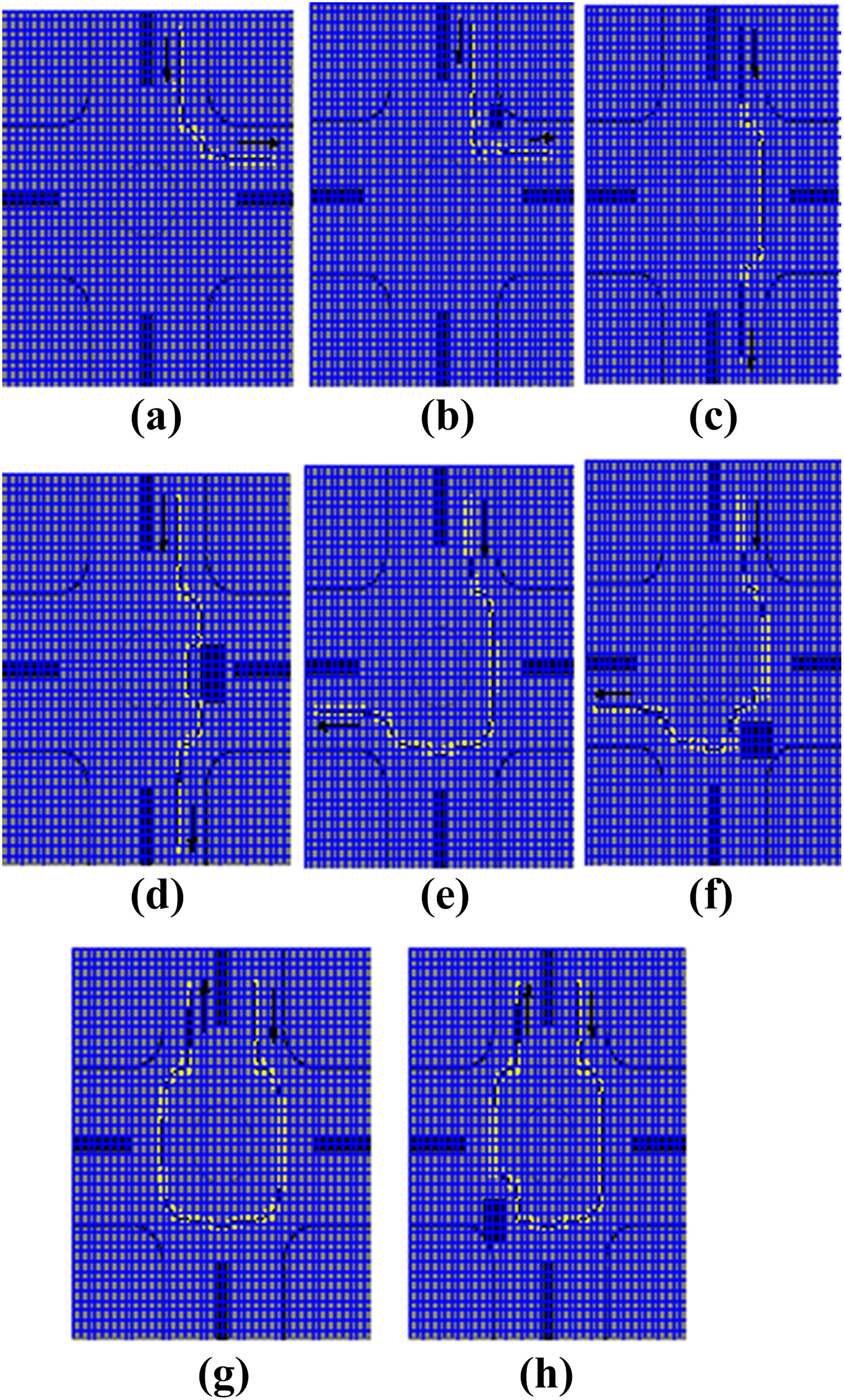
LS path planning (yellow colour) starting from the entrance at the top of the roundabout environments (black colour): (a) Left Rot. −90° Left, (b) Left Rot. −90° Left with obstacle, (c) Left Rot. −180° Straight, (d) Left Rot. −180° Straight with obstacle, (e) Left Rot. −270° Straight, (f) Left Rot. −270° Straight with obstacle, (g) Left Rot. −360° Straight and (h) Left Rot. −360° Straight with obstacle.

Simulation results for various scenarios

Figure 8 shows the simulation of the robot path when travelling from start to goal positions in the roundabout considering eight scenarios. The path from each entrance is generated to determine the appropriate branch exit: Left Rot. −90° Left, Left Rot. −180° Straight, Left Rot. −270° Straight and Left Rot. −360° Straight, each of them is represented with the presence of obstacle or in collision-free path.

Part B: Local path planning in the real road roundabout environments

LS is used in the real roundabout environments to determine if the roundabout is located within the local 2D map that is constructed from the camera and image processing algorithm during mobile robot navigation in roundabout environments. The LS algorithm is quite similar to the one that has been previously discussed in part A, with some minor changes:

– Local path planning deals with live streaming video not just one static image as in the global case.

– The roundabout centre in the video image sequences is looked upon as an ellipse not as a circle unlike in part A.

– The dimension of the roundabout could not be computed due to the image scaling system of the camera and calibration error.

To evaluate the local path planning using LS in roundabout detection, experimental works have been carried out to find the collision-free path in a real roundabout with cylindrical obstacle as follows:

i. Real roundabout

The LS algorithm is used to apply robot’s navigation in the real road roundabout as shown in Figure 9.

Figure 9.

Sequence of images produced by the LS algorithms for real roundabout navigation: (a), (e), (i) and (m) – original images; (b), (f), (j) and (n) – images from the preprocessing and processing operations; (c), (g), (k) and (o) – applying the LS algorithm (represented by continuous or discontinuous lines in the middle); (d), (h), (l) and (p) a comparison between LS (black) and PB algorithm (red). LS: laser simulator; PB: PointBug.

It has been seen that the algorithm manage to effectively detect the roundabout when it is detected from the sequence of images as shown in Figure 9.

The continuous lines in the middle of the LS images as shown in Figure 9(c), (g), (k) and (o) results denote that the roundabout is still not detected and the robot should continue moving with the same speed. However, the discontinuous line shown in Figure 9(l) indicates the detection of the roundabout upon which the robot must change its speed and start moving in a circular path within the roundabout.

The LS is compared with PB algorithm ¹⁷ as shown in Figure 9(d), (h), (l) and (p) to evaluate the performance of the LS in the local maps. The PB algorithm has a range equals to 1 m in this work.

From Figure 9(d), (h), (l) and (p), it is obvious that the paths produced by LS and PB are similar in which the roundabout is still located far from the current position. However, the PB approach has a noticeable drift when the roundabout is detected in its measurement range. This is because the PB algorithm depends on the obstacle edges to determine the path of the robot, whereas LS depends on each sequence of measurements to find its path.

• ii. Cylindrical obstacles

The roundabout detection algorithm is also tested by placing a cylindrical obstacle in the robot path. The LS shows its capability to distinguish between the obstacle and the roundabout and determine the path as shown in Figures 10 and 11. The path navigated through the LS is compared with PB algorithm as shown in Figures 10 to 12(c).

Figure 10.

LS path with cylindrical obstacle in the middle of road: (a) original image; (b) image from the preprocessing and processing operations; and (c) applying LS algorithm (black) and PB algorithm (red). LS: laser simulator; PB: PointBug.

Figure 11.

LS path with cylindrical obstacle near the right curb of the road: (a) original image; (b) image from the preprocessing and processing operations; and (c) applying LS algorithm (black) and PB algorithm (red). LS: laser simulator; PB: PointBug.

Figure 12.

LS path with cylindrical obstacle near the left curb of the road: (a) original image; (b) image from the preprocessing and processing operations; (c) applying LS algorithm (black) and PB algorithm (red). LS: laser simulator; PB: PointBug.

Similar to the fifth section, part B(ii), LS shows good performance in comparison with the PB algorithm since the PB uses few points to find its path and always connect the path to the obstacle edges, which resulted in non-smooth and fluctuating paths as shown in Figures 10 to 12(c).

• iii. Roundabout navigation and path determination

A WMR platform with three wheels actuated by differential drive motors has been used to inspect the LS algorithm in real road roundabout environment as shown in Figure 13. It is a medium size platform with gross mass (105 kg) and dimensions (100 × 70 × 30 cm³) and can move at a relatively low speed, typically in the range of [0.2, 1.5] m/s. It consists of three main units: differential drive, measurements and vision and processing units. An on-board computer is used as a host controller, where the LRF and Wi-Fi camera are connected directly to the PC and two DC motors with encoders are connected via dual brushless cards (Interface Free Controller IFC-BL02) to motor driver card (MDS40A) and brush cards (IFC-BH02), respectively, through the computer interface card (IFC-CI00). The main power card (IFC-PC00) regulates the power supply to the whole embedded controller system.

Figure 13.

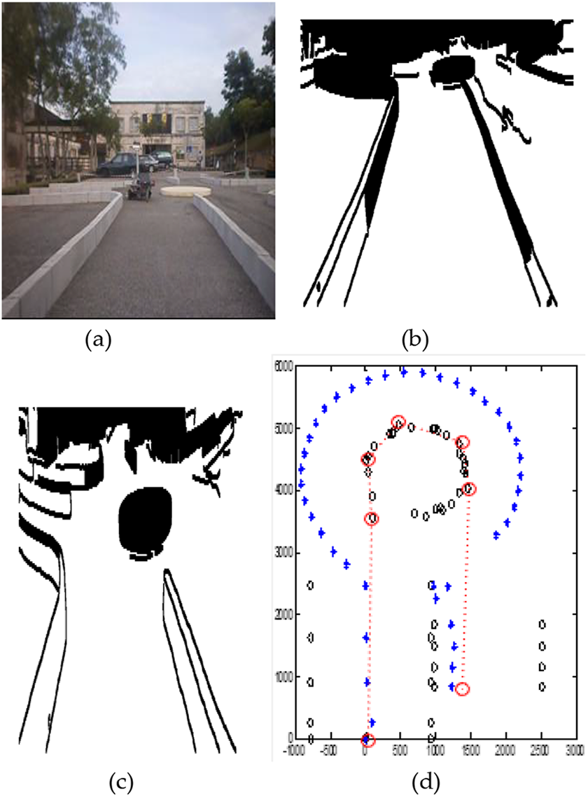
Outdoor mobile robot navigation using LS: (a) image showing the mobile robot platform and roundabout environments, (b) camera’s local map for LS when the robot starts moving, (c) camera’s local map for LS when the robot detects the roundabout and (d) path of mobile robot when navigating in a roundabout setting (black circle) using LS and sensors fusion (blue crosshairs) in comparison with the PB algorithm (red circles and are connected by the red dotted) within roundabout setting (6 m length and 4 m width). LS: laser simulator; PB: PointBug.

The interface computer card (IFC-IC00) is the main controller that imports and exports the data from host computer to the slave IFC card via stacker pins. The slave IFC cards (IFC-BLO2, IFCBH02) are configured to the main controller using a unique communication addresses. Visual C# is the main processing program for IFC cards and MATLAB is used for the video and signal processing acquired from the camera and LRF, respectively, since it has suitable image and signal toolboxes. The linking between C# and MATLAB was done using the COM automation server; data can be created in the client C# program and passed to MATLAB and vice versa.

The LS with camera’s local map parameters is incorporated with the LRF and encoders for roundabout detection and navigation from starting position at specific entrance of the road to the target position that is located in a specific exit of the roundabout with a path equals to 20 m as shown in Figure 13. The LS path is compared with the PB counterpart to find the collision-free path in road roundabout as shown in Figure 13(d).

The path planning of the robot using LS looks smooth in the road following and roundabout regions as shown in Figure 13(d). However, there is a slight drift (deviation) in the navigation path near to the entrance and exit of the roundabout due to the increasing of the robot speed which could not be controlled since it is merely a path planning methodology and no control scheme is employed at this point in time. Other reasons are related to the LRF inaccuracy and sensitivity while measuring the static objects (curbs and roundabout centre) and non-symmetrical entry and exit features in the roundabout. On the other hand, the PB algorithm has detected the roundabout as an obstacle and generates the path using the start point, five interconnected points in the roundabout and goal point which eventually cause the robot to ‘crash’ undesirably at certain points within the roundabout as shown in Figure 13(d).

Conclusion

A novel algorithm, the so called LS to determine a collision-free trajectory in an unknown environment has been presented. With this approach, it is possible to apply several constraints in the robot path while navigating in a complicated terrain such as a road roundabout environment. Other conclusions that can be drawn are as follows:

The main advantage of this approach is the LS ability to be used for both global and local path planning with the presence of obstacle and unknown environment.

A case study on its implementation in both global and local path planning has been applied in a road roundabout setting.

In the global path planning, the path is generated within the grid map of roundabout environment to select the path according to the respective road rules. It is also used to recognize the real roundabout and generate the path from sequence of images during the local path planning in real-world circumstances.

Results show the effectiveness of this approach in both simulation and experimental set-ups. The LS approach has been compared with other well-known approaches, namely the A*A, VDFM and PB algorithm to show its path performance when implemented in both global and local path planning environments.

Future works shall include the implementation of LS for the mobile robot to navigate in other more challenging and complex environments and the possibility of embedding a robust control method to enhance its overall navigating and controlling performance.