
Abstract
In this article, a distributed model-free consensus control is proposed for a network of nonlinear agents with unknown nonlinear dynamics, unknown process disturbances, and white noise measurement disturbances. Here, the purpose of the control protocol is to first synchronize the states of all follower agents in the network to a leader and then track a reference trajectory in the state space. The leader has at least one information connection with one of the follower agents in the network. The design procedure includes adaptive laws for estimating the unknown linear and nonlinear terms of each agent’s dynamics. The salient feature of the proposed control scheme is that each agent’s estimation is a model-free adaptive law, that is, the need for regressor or linear-in-parameter basis is alleviated. In addition, without requiring direct connection to the leader, the leader’s control input can still be reconstructed by virtue of a robust observer which can be defined in a distributed manner in the network. The entire design procedure is analyzed successfully for the stability using Lyapunov stability theorem. In addition, it is shown that the proposed distributed controller includes an optimal term. Besides, a modified Kalman filter is added to eliminate the measurement noise. Finally, the simulation results on three networks of unknown nonlinear systems are presented. Moreover, a comparative study is presented to evaluate the proposed algorithm against a model-based cooperative control algorithm.
Keywords
Introduction
Great attention has been paid to the problem of controlling multiagent systems ranging from consensus to formation control. 1 –4 The solutions applied to oscillator synchronization, mobile robot and aircraft formation, mobile sensor area coverage, vehicle routing in traffic, containment control of moving bodies, and so on. 5 Generally, all of these problems can be considered as a consensus problem, in which all agents’ states (or outputs) should be synchronized inside a network. 6 In practice, each agent’s dynamics usually has an unknown nonlinear structure due to unpredictable environmental disturbances, unmodeled dynamics, and other uncertainties. Hence, the requirement for designing distributed cooperative control without any a priori model of the agents’ dynamics is essential. These types of control policies are called model-free controllers (MFCs) 7 or data-driven controllers 8 in the literature. Although several MFCs have been proposed for a single-agent system, 7,9 –14 the use of MFCs for multiagent systems is quite new. 15,16
The consensus problem for a class of nonlinear first-order multiagent systems with external disturbances is discussed by Das and Lewis, 17 while the problems for second-order and higher-order nonlinear multiagent systems are reported by Zhang and Lewis 1 and Peng et al., 2 respectively. Distributed adaptive leader-following control for unknown dynamic systems with guaranteed finite-time convergence is proposed by Mahyuddin et al. 18,19 The algorithms are model-based cooperative controllers which require sufficiently rich input signals to guarantee persistently excitation condition for the regressors. The procedure to design a distributed state–output feedback cooperative control is presented by Wang et al. 20 for uncertain multiagent systems in undirected communication graphs. This procedure is extended for a directed communication graph with a spanning tree characteristic. 21 To remedy the problem of a non-affine system for a general class, several works such as by Meng et al. 22 employ a direct adaptive approach using an artificial neural network (ANN).
Most of the MFCs for nonlinear systems in the literature are proposed under the context of reinforcement learning (RL). These controllers are actually optimal adaptive controllers, which calculate the optimal control policy in an online manner using some adaptive laws. 23 These algorithms include an online estimation process for the cost function to evaluate the controller performance (critic network) and another online process to estimate the optimal control signals (actor network). These two online estimations are performed using two distinct ANNs. 24 While more appropriate performances can be achieved by increasing the number of nodes in each of the mentioned ANNs, this may increase the computational complexity. 25 Future prospective applications may be limited due to this caveat especially involving scarce energy resources. If the MFCs do not include ANNs for online estimation, the number of adaptive laws is reduced and the problem of computational complexity would be eliminated. Such an attractive feature, that is, being lite in computation, opens up multiple possibility of having the control scheme deployed on any distributed system.
A robust adaptive cooperative control is proposed by Mahyuddin and Safaei 26 for formation-tracking problem, whereby the system matrix for dynamic system is assumed to be known. In this article, however, the system matrix is completely unknown and to be estimated with a model-free adaptive law. In contrast to the previous work by Mahyuddin and Safaei, 26 the main controller gains are, instead, determined online. Another salient feature exemplified in this article is that the proposed cooperative controller considers an optimal policy by virtue of RL to find a solution to the algebraic Riccati equation.
Safaei and Mahyuddin 27 proposed the idea of model-free cooperative controller for the first time. By contrast, here an optimal analysis is also provided to show that an optimal term is incorporated into the proposed controller. Moreover, a detailed explanation about the dynamical structure for unknown dynamics of each agent in the network is presented in the current work. The approach adopted does not require the maximum absolute values for unknown dynamics of each agent.
In this article, a distributed consensus control problem is solved for a network of agents with general unknown nonlinear multi-input and multi-output (MIMO) dynamic system using a model-free control algorithm. The main contribution of this article is the design and development of an MFC algorithm for consensus problem involving a network of nonlinear multiagent systems without requiring the use of ANNs to estimate the unknown system dynamics and disturbances. Here, the proposed distributed MFC is based on a new structure for the unknown dynamics of each agent. The unknown dynamics of each agent can be segmented into two parts: linear-in-states and nonlinear. Two separate adaptive laws are proposed for estimating both linear and nonlinear terms in the system at each agent. The estimation of unknown nonlinear terms is performed in such a way that the dependence on any model regressor or nonlinear basis functions is removed. This implies that the estimation is regressor-free. By estimating the linear terms, a technique is proposed for online determination of the controller gains locally at each agent by the solution of a continuous-time algebraic Riccati equation (CARE). Moreover, a robust observer is designed for all the follower agents, which are not connected to the leader. The observer estimates the leader’s control input(s). The stability analysis of the whole algorithm is provided with Lyapunov stability theorem. In addition, an optimality analysis based on the solution of a Hamilton–Jacobi–Bellman (HJB) equation is presented to illustrate the efficacy of the optimal term in the proposed cooperative MFC controller. Furthermore, since the proposed structure for unknown dynamics of each nonlinear agent in the network is linear-in-states, a modified Kalman filter is implemented to remove the measurement white noise. Finally, a simulation study is provided to evaluate the performance of the proposed distributed controller on a chaotic plant and a non-affine nonlinear system. The contributions of this article are listed as follows: A distributed MFC protocol is proposed for a generic unknown nonlinear system without the use of any ANN. The network-based adaptive law for estimating the unknown nonlinear terms at each agent is regressor-free. The controller gain (P matrix) is updated online without requiring knowledge on the communication topology of the network.
In the following, first, a general formulation for a network of unknown nonlinear agents is proposed in General formulation for a network of unknown nonlinear MIMO agents. The design procedure for the MFC cooperative control is presented in Design procedure for model-free cooperative control with tracking objective. That section includes three different subsections dedicated to distributed estimation for unknown system matrix, adaptive MFC cooperative protocol, and cooperative robust observer for the leader’s control inputs. In Cooperative robust observer for leader’s control inputs, the modified Kalman filter observer is proposed for compensating the measurement noise. Finally, a simulation study including three different cases, a comparative study against a model-based cooperative control algorithm, and an analysis for different types of measurement noise are provided in Observer design for compensation of measurement noise, Simulation study, and Comparison with model-based cooperative control algorithms, respectively.
General formulation for a network of unknown nonlinear MIMO agents
Definition 1
Consider a network of N homogenous nonlinear dynamic systems. Let

to represent the interagent communication link (inclusive of the leader pinning) to be exploited in the analysis of this article.
Assumption 1
Here, the necessary condition about the network is that at least one of the agents should have the communication link with the leader. In other words, at least one of the diagonal elements in matrix
Definition 2
Consider the network defined in definition 1. A general unknown nonlinear dynamic system for ith agent can be defined as

where

where

The only minimal information required about the dynamic system of each agent is to know whether each system states depends on each of the control inputs or not. The matrix B can be constructed by this information according to equation (4). Finally, by considering

the unknown nonlinear system in equation (2) can be presented as

where
Definition 3
For a network of N agents with dynamics defined in equation (6), we can have the dynamic expression for the whole network as

where
Definition 4
Let us define dynamics of a virtual leader for the network introduced in definition 2 as
Definition 5
For a network defined in definition 1 to definition 4, we can define a consensus error

The consensus errors of all agents in the network can be expressed as

where
Design procedure for model-free cooperative control with tracking objective
Distributed robust adaptive parameter estimation for unknown system matrix
Lemma 1
Combination of a stable estimator and a stable controller within a dynamic system will lead to a stable system. This is investigated in the literature as separation principle for both linear and nonlinear dynamic systems. 29,30
Theorem 1
Consider the dynamics of agent i in the network as in equation (6). If one can define

as the rate for estimation of A at ith agent, where λ is a positive scalar and

and
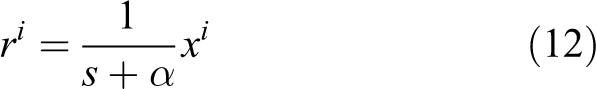
where s is the Laplacian operator and

the filtered format of H0 defined as

converges to zero asymptotically.
Proof
Let us define the estimation error for Ai as

Then, by filtering both sides with

which is in the form of

consequently leading to

Now, consider the following Lyapunov function

which has derivative as

To have

It should be noted that according to definition 2, the elements of A are constant real values; hence
Proposition 1
The adaptive law, estimating the linear term A, is equipped with a leakage term to make the estimation robust against bounded perturbation 31 as follows

where ρ1 is a positive scalar.
Remark 1
Referring to theorem 1, the values of
Remark 2
Referring to lemma 1 and theorem 1, one can replace

Distributed adaptive MFC protocol
In this section, two analyses are presented for designing the distributed adaptive MFC protocols. They are stability analysis and optimality analysis.
Stability analysis
Proposition 2
If the consensus errors of all agents as in equation (9) converge to zero, then all agents in the network will synchronize to each other and to the reference trajectory denoted by the leader agent successfully, that is,
Theorem 2
For a network with dynamics defined in equation (7) and recalling the consensus error in equation (9), with providing the conditions that the diagonal elements in

where

where γ is a positive constant scalar defining the adaptation rate and ρ2 is another positive scalar acting as the leakage term, then proposition 1 will be achieved.
Proof
Consider the following Lyapunov function
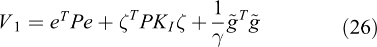
where
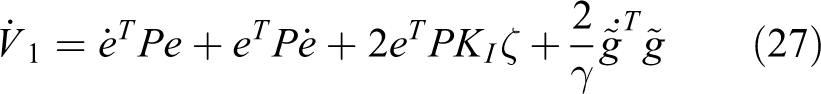
leading to

By replacing

Besides, by multiplying both sides of equation (9) with

In addition, by recalling remark 1 and the undirected property for the communication graph of the network (which in turn means that matrix

Thus, by incorporating equations (30) and (31) into equation (29) and recalling the mixed-product property for Kronecker product, substituting

Since

Then, by adding and subtracting

we lead to

Utilizing the following adaptive law

the third term in equation (35) is zero. Hence, we have

Since g is bounded and Lipschitz, we have

where

Note that Λ1 and δ1 are two positive constant scalars. Besides, if we set

where

Further, by setting

for Q > 0 in

where

According to the LaSalle–Yoshizawa theorem, V1 is uniformly ultimately bounded. Since V1 includes the tracking error and the estimation error, we can deduce that e and its time integral ζ and also

Then, by rearranging this equation and recalling that B is full-rank and
Remark 3
According to equation (42), the controller gains Pi can be determined online using the solution of following CARE

It is significant that the solution of this equation does not depend on the communication graph (i.e.
Optimality analysis
Definition 6
Referring to the proposed formulation in definition 4 for a network consisting N continuous-time nonlinear agents, one can define the following cost-to-go function 32

for measuring the performance of a designed set of distributed control inputs u regarding the consensus-tracking objective. Here, V4(.) is a scalar cost according to the performance of the system in future operations and J(.) is a scalar value named system’s utility.
Proposition 3
Based on the HJB equation, the optimal control for the dynamic system proposed in equation (23) should satisfy 32

Theorem 3
For the consensus problem defined in proposition 1, if one can construct the following cost function

and the following utility function

where

then it can be shown that the distributed controllers proposed in equation (24) include the optimal policies.
Proof
Since the dynamics of agents is proposed in a linear format as in equation (23), one can conclude that the cost-to-go function J for this system can be represented as quadratic functions of system states. 32 Hence, equation (49) can be defined. Besides, by recalling lemma 1, remark 2, and theorem 2, one can represent equation (23) as

For the defined V4 and J in equations (49) and (50) and referring to equation (48), the following Hamiltonian is proposed

By replacing

we have

Moreover, by replacing

Then by recalling the mixed-product property for Kronecker product, we have

At this point, we redefine u in equation (40) as

and

By recalling

Then by recalling equations (30) and (31), we have

or

which is equal to zero by determining the values of P from the CAREs in equation (46). In addition, by differentiating H3 with respect to u1, we have

This equation is equal to zero by substituting u1 from equation (58). It means that a part of u is designed in such a way that the partial derivative of H3 is zero. Then by referring to proposition 3, the optimality condition is satisfied and the proof is completed.
Cooperative robust observer for leader’s control inputs
Remark 4
Looking at equation (24), the controller input at the neighboring agent (i.e. uj) is required for computing ui. But, this value is not available, since it is being computed at the same time. Thus, the need for an estimation algorithm for uj is invoked.
Theorem 4
For a network defined in definitions 1 and 2, if proposition 1 is satisfied by theorem 2, then one can have the following approximation for relation between the control inputs at agent j and the leader’s control inputs

Proof
Recalling lemma 1 and theorem 1 and also by subtracting both sides of

Then, by reaching consensus on synchronization and tracking problem (according to theorem 2), one can state that

Using the time derivative of both sides of this equation, we have

Finally, the approximated value for controller inputs of agent j can be expressed as follows

Then the proof is completed.
Remark 5
Utilizing theorem 4, one can use equation (64) to compute the designed control inputs in equation (24). But, considering the pinning gain matrix
Proposition 4
Referring to the objective of reaching consensus on observation for values of u0 at all agents in the network, one can define the following consensus error
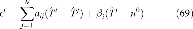
where

where
Theorem 5
For a network defined in definitions 1 and 2 with at least one communication connection between the leader and the agents in the network, if one uses the following equation as the rate for observing the leader’s control input
where μ is a positive scalar,
Proof
Considering the following Lyapunov function

we have

Since the summation of all elements in each row of the Laplacian matrix is zero, 5 we have

Hence, equation (73) can be written as

Considering

In the case that the communication graph is connected and undirected and

where

To achieve

Then, since

At this point, we should only show that

Thus,

Finally, since

we have

and then the rate for observed parameter is

Using
Remark 6
Recalling proposition 1 and theorems 2, 4, and 5, the distributed controller at agent i in the network is proposed as

where

and Pi is the solution of following CARE

Remark 7
It should be noted that the number of estimations (excluding the number of observers for the leader’s control inputs) at each agent in the network is equal to the number of adaptive laws for
Observer design for compensation of measurement noise
Looking at the considered dynamical structure at each agent as in equation (6), one can implement a linear Kalman filter at each agent as an observer on the proposed distributed model-free control protocol to remove any possible bounded measurement noise. This forms one of the primary motivations for the expressed dynamical structure in equation (6) to have a linear-in-states term.
Proposition 5
Suppose that there is a source of white noise on each measured states of agent i. Hence, using the adapted parameters in equation (6), the dynamics of agent i in the network can be represented as

where
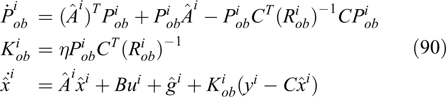
Here, η is a positive tuning gain defined to provide fast and accurate performance for the modified observer. It is shown in the study by Lewis et al.
33
that using equation (90), the observer error, that is,
Simulation study
In this section, three applications for the proposed consensus control protocol are presented. First, we studied the performance of the controller on a network including four chaotic plants. Then, the controller is evaluated on another network of non-affine nonlinear plants. The third simulation case is dedicated to a network including four limit cycle resonators. In these three applications, the properties of the communication graph and the constant parameters of the controller are considered to be the same. The communication network in each case consists of four agents with different initial values for the system states. The adjacency and pinning gain matrices for the communication graphs are

In addition, the controller parameters at agent i in the network are tuned, as presented in Table 1. These values are used for all of the following simulation cases, otherwise it is mentioned specifically. In Table 1, I2 is an identity matrix with dimensions of two. Moreover, in the following simulation cases, matrix B is assumed to be I2. Here, a normally distributed random noise with mean value of zero and variance equal to 0.5 and 0.05 is added as the measurement noise to the first and second states, respectively, at each agent for all of the simulation cases.
Controller parameters at agent i.

Case 1: Chaotic plant
Here, a network consisting of four Duffing–Holmes chaotic systems has been considered for evaluating the performance of the proposed controller. The dynamics of a single-agent Duffing–Holmes chaotic system is 34

where

Case 1: Values for first state (x1) for all agents. The initial values for states of all agents are not identical. The consensus of states for all agents to the desired trajectory can be confirmed after about 2 s.

Case 1: Consensus errors of first state for all agents. It can be seen that the consensus errors for agents (ei) are bounded around zero with the upper-band value of about 0.35.

Case 1: Control inputs for all agents. The control variables for all agents are also bounded.
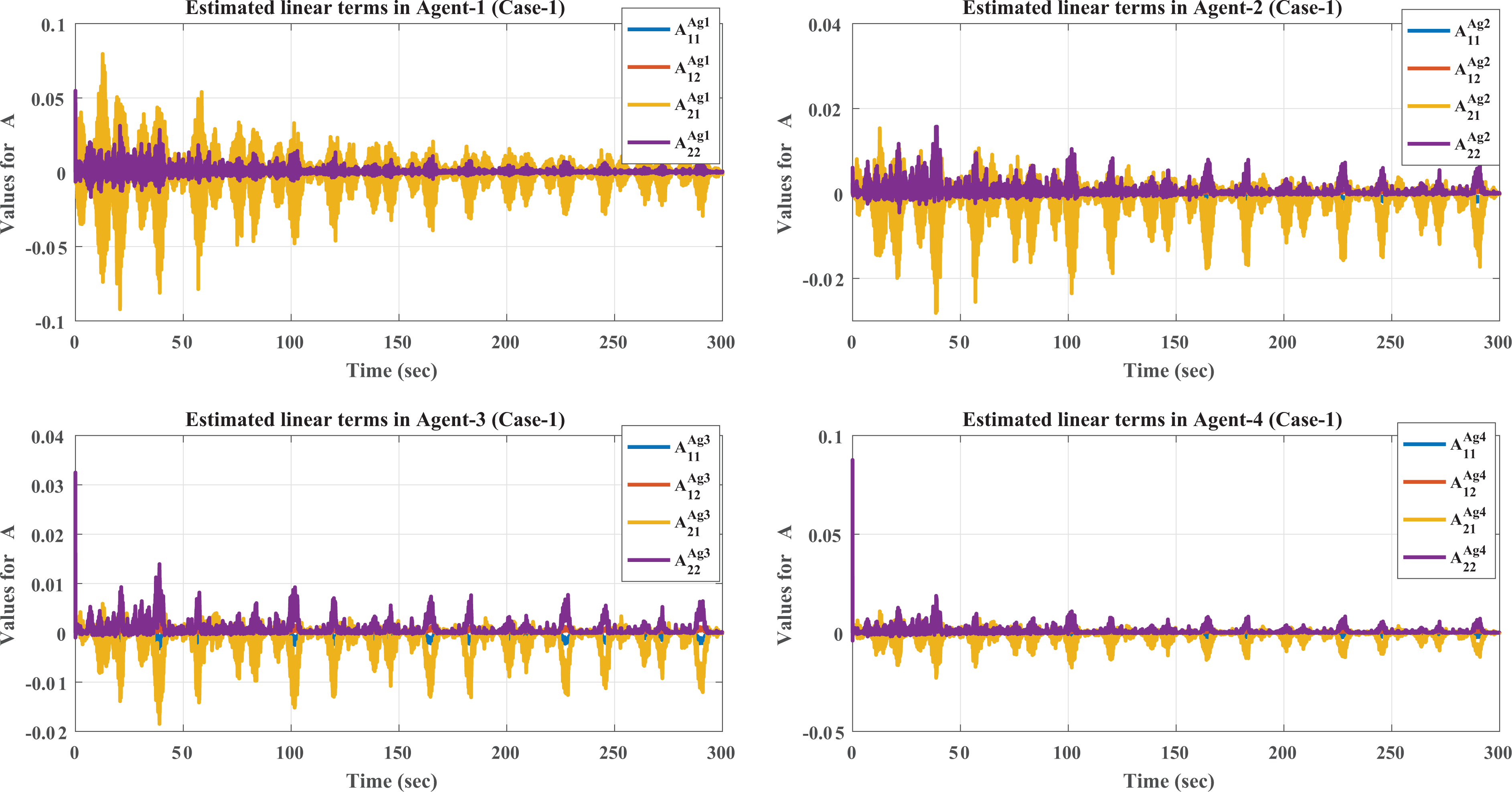
Case 1: Estimated values for linear terms (
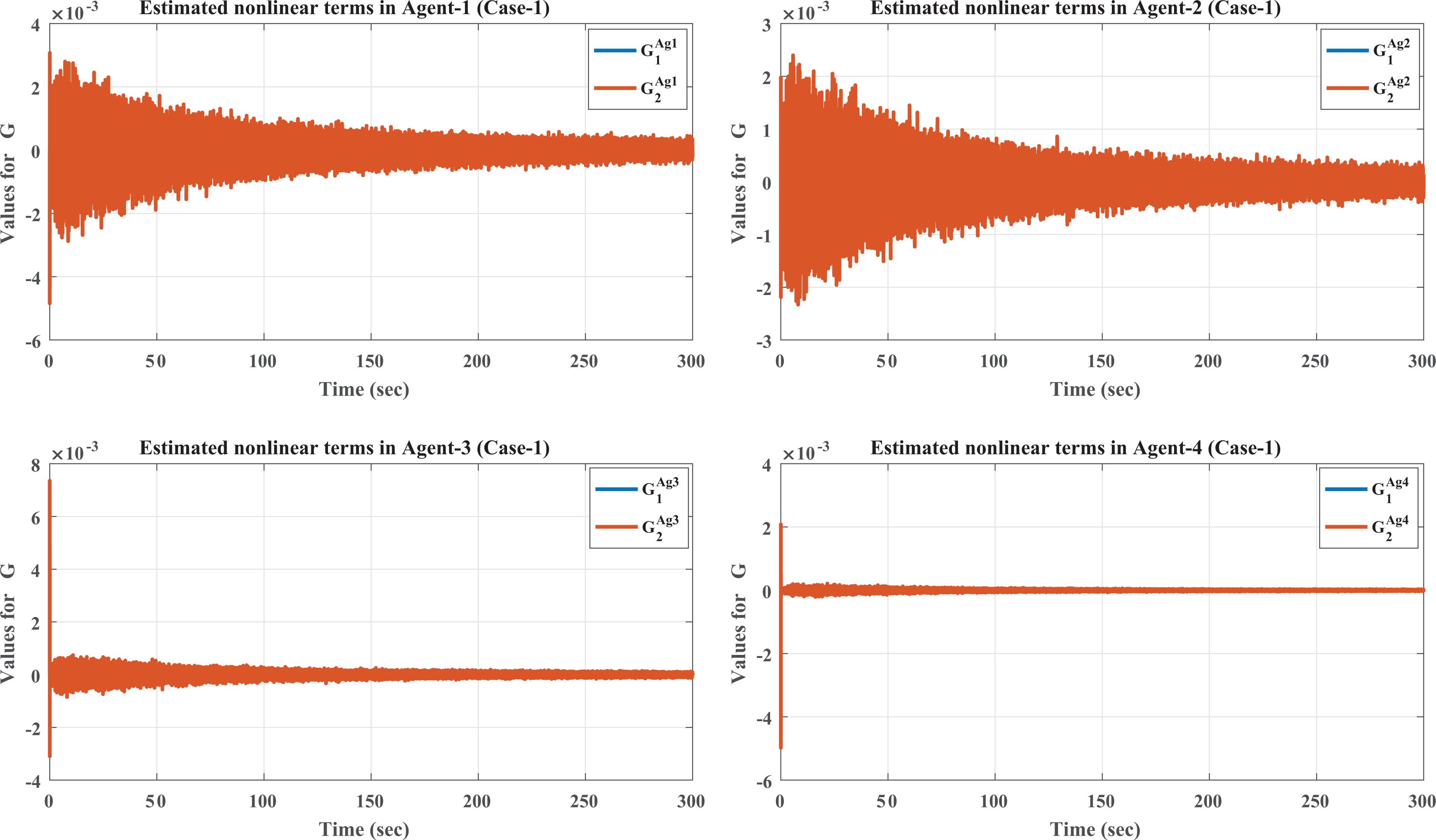
Case 1: Estimated values for nonlinear terms (

Case 1: Observed values for the leader control input (
Case 2: Non-affine nonlinear system
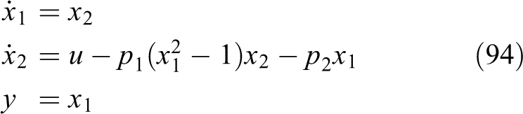
The dynamic system in this simulation case is 35

The system defined in equation (93) is a non-affine system. The desired value for the first state is zero for all agents, which are starting the simulation at different nonzero initial values. The dynamic system can be formulated as in equation (6) with two states. In addition, the controller parameters are set as suggested in Table 1, except the value of Ki which is equal to

Case 2: Values for first state (x1) for all agents. The initial values for states of all agents are not identical. The consensus of states for all agents to the desired trajectory can be confirmed after about 3 s.

Case 2: Consensus errors of first state for all the agents. It can be seen that the consensus errors for agents (ei) are bounded around zero with the upper-band value of about 0.3.

Case 2: Control inputs for all agents. The control variables for all agents are also bounded.
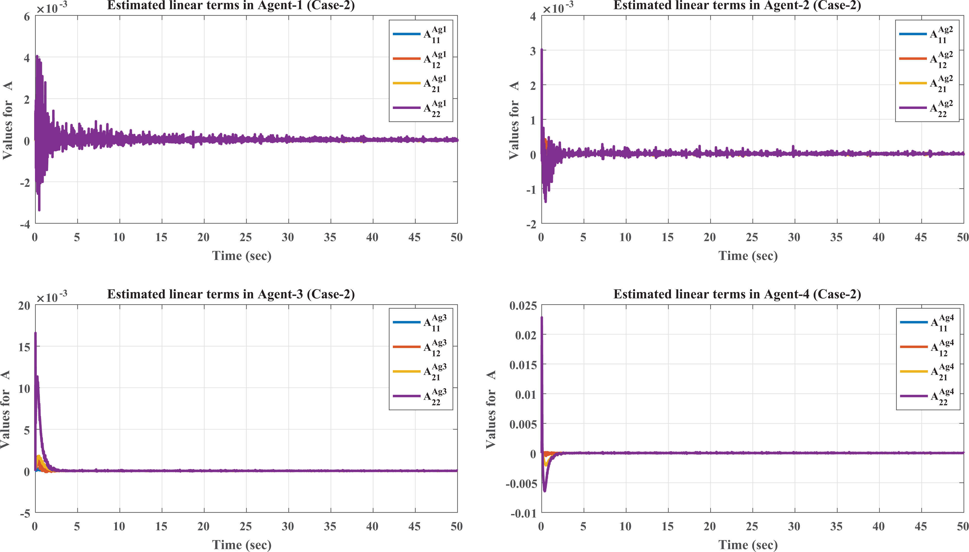
Case 2: Estimated values for linear terms (

Case 2: Estimated values for nonlinear terms (
Case 3: Limit cycle resonator
For the third case, a limit cycle dynamic system is considered for the dynamics of each agent in the network. The dynamic system for a Van der Pol resonator as a limit cycle dynamic system is proposed as follows 36
where p1 and p2 are two positive constant values. This simple dynamic system has a stable equilibrium point at (0, 0). In addition, the system has an unstable limit cycle surrounding the origin. 37 The unstable limit cycle represents the boundary between the transients which converge to the origin and those transients which diverge. 37 In this simulation, we consider p 1 = 0.1 and p 2 = 0.2. The simulation results for this case are presented in Figures 12 to 17. It can be seen that the states for all agents are converged to the desired value of 3, although the initial values for the states of agents are not the same. The convergence trends of the observed values of the leader control input in different agents are almost the same (see Figure 17). Moreover, the tracking errors and the control inputs are bounded.

Case 3: Values for first state (x1) for all agents. The initial values for states of all agents are not identical. The consensus of states for all agents to the desired trajectory can be confirmed after about 3 s.

Case 3: Consensus errors of first state for all agents. It can be seen that the consensus errors for agents (ei) are bounded around zero with the upper-band value of about 0.4.

Case 3: Control inputs for all agents. The control variables for all agents are also bounded.
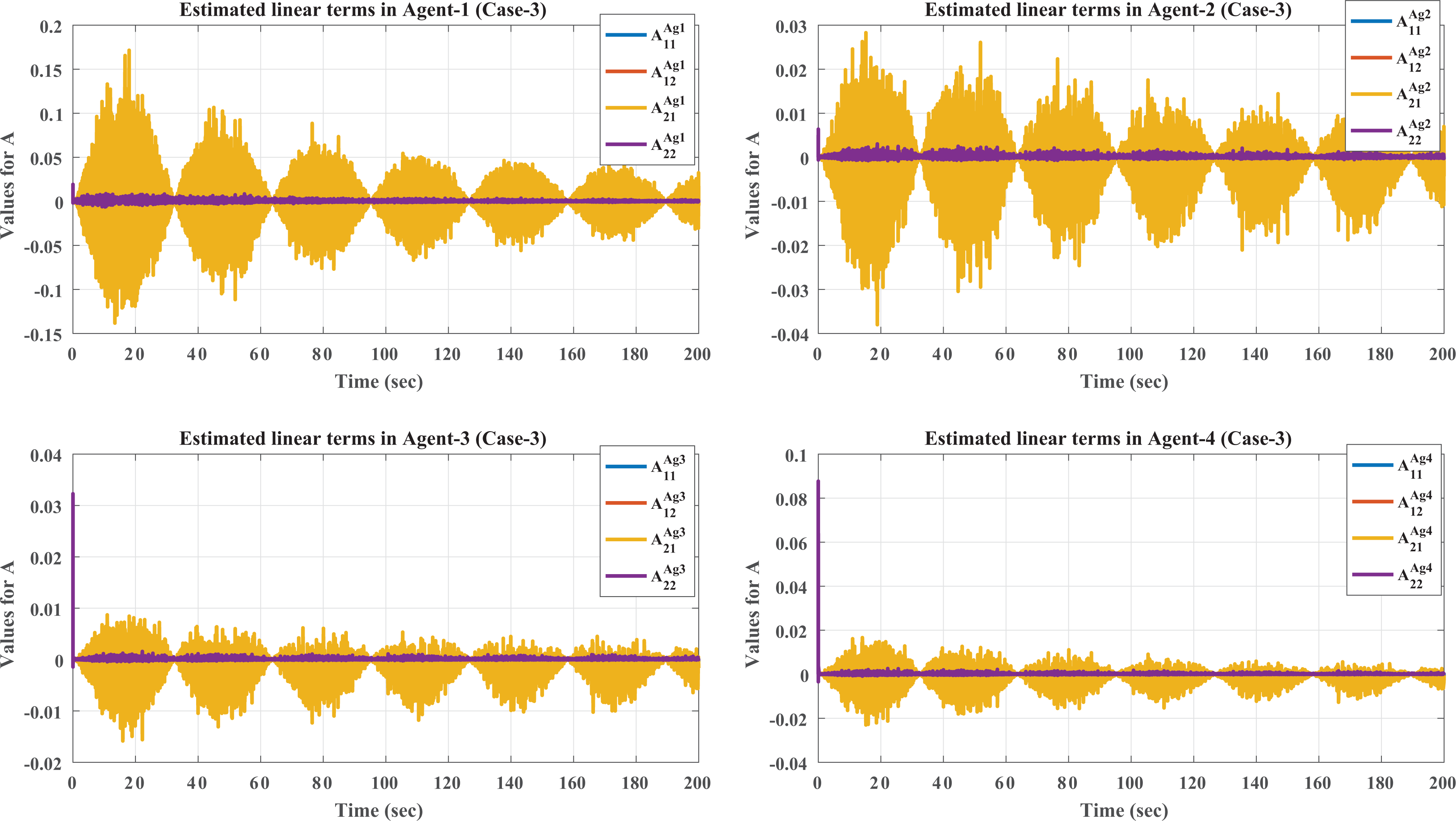
Case 3: Estimated values for linear terms (

Case 3: Estimated values for nonlinear terms (

Case 3: Observed values for the leader control input (
Comparison with model-based cooperative control algorithms
In this section, the performance of the proposed model-free cooperative control algorithm (remark 6) is compared with a well-known model-based cooperative control algorithm designed and presented by Lewis et al. 5 The control signal at agent i in this algorithm is defined as follows 5

where di and βi are defined in definition 1 and

In the above two equations, Wi is —the vector of gains for the employed neural nodes at agent i, while ϕi is the basis for activation functions of neural nodes.
5
Moreover, c, λ, F, and k are constant parameters for tuning the control algorithm. The values for pi are defined based on the solution of a Lyapunov equation.
5
The algorithm is designed specifically for the unknown second-order dynamic systems, where
The dynamic system for the comparison study in this section is a reverse pendulum presented with the following model 5

where Jp, Mp, and Lp are the moment of inertia, mass, and the length of the pendulum, respectively. In addition, g is the gravitational acceleration and Bp is a constant for damping force. Here, we have a network of five agents with the dynamic system as presented in equation (97) at each agent. The communication graph in this network is presented in Figure 18 and only the third agent is pinned to the leader.
5
The desired value for x1 of all agents in the network is

The communication graph of the network considered for the comparison study. It has five agents (nodes) with one leader pinned to the third agent. 5
By contrast, the constant values of the proposed model-free cooperative control algorithm are chosen same as the values in the simulation case studies (Table 1), except

is used to compute the total absolute effort
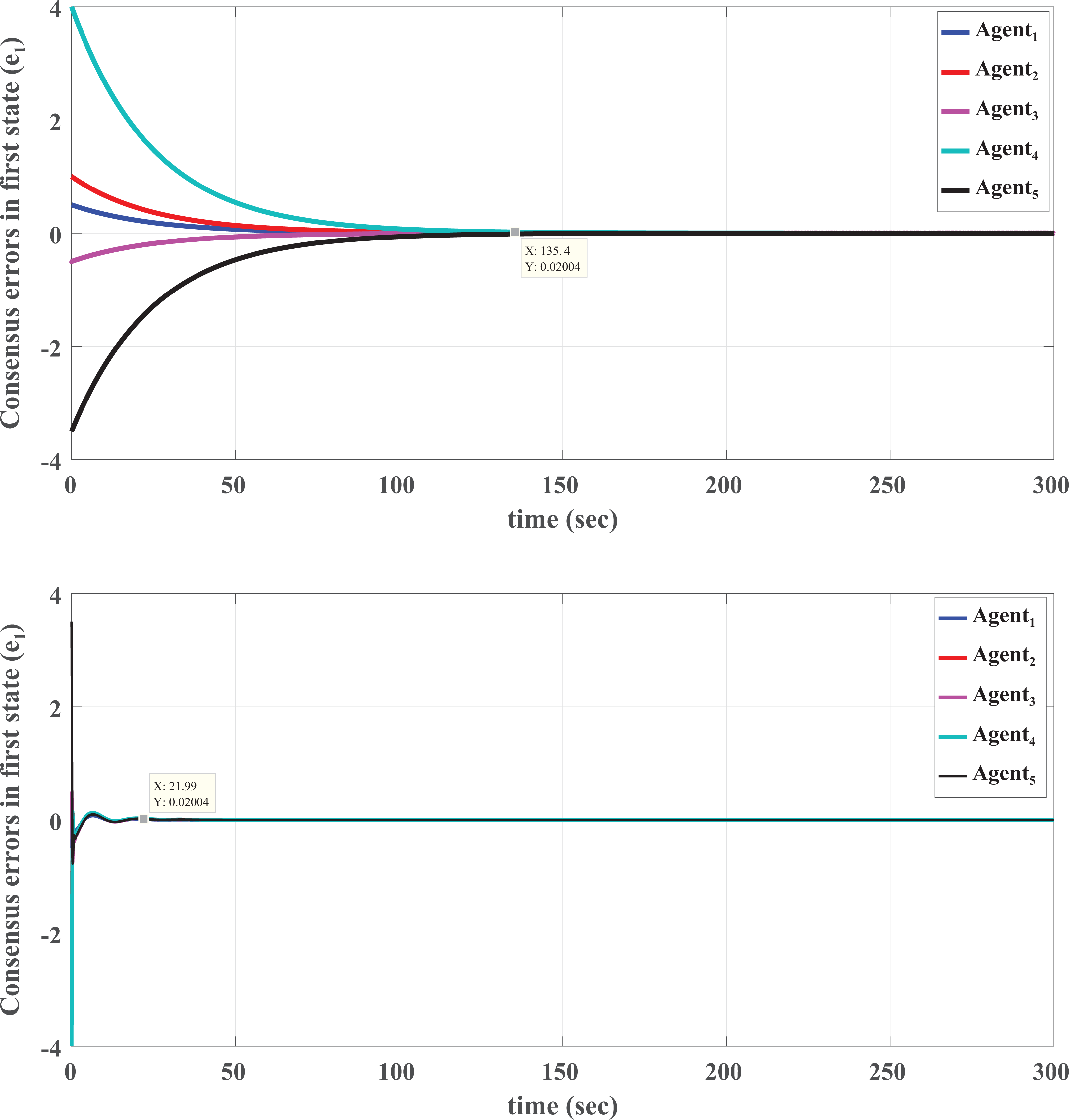
Comparison study: The consensus errors for all agents using the model-based (top) and model-free (bottom) cooperative control algorithms. The convergence is provided in both cases, while the model-free algorithm is a bit faster and has extra overshoot.

Comparison study: The values for first states of all agents using model-based (top) and model-free (bottom) cooperative control algorithms.
Total absolute control effort at agent i.

Analysis for different type of measurement noise
As it is mentioned in proposition 5, the proposed observer is designed with this consideration that the measurement noise is a normally distributed random system. In this section, the performance of the proposed joint controller and observer system is evaluated under the assumption of the existing uniformly distributed noise (instead of normally distributed noise) on each state of all agents in the network. In this regard, the simulation results for case 1 are computed again with considering the above assumption. Here, a uniformly distributed measurement noise with maximum value of 0.5 and minimum value of −0.5 is implemented on the first state. The implemented noise on the second state is less by a factor of 0.1. As it is shown in the plots in Figures 21 and 22, the convergence is achieved appropriately and the errors are all bounded. Based on these results, one can say that the proposed distributed adaptive model-free cooperative control algorithm and the observer in proposition 5 have acceptable performance in the case of uniformly distributed measurement noise.

Values for first state (x1) for all agents in case 1, under the assumption of uniformly distributed measurement noise. The convergence to the desired trajectory is provided for all agents.

Consensus errors of first state for all agents in case 1, under the assumption of uniformly distributed measurement noise. The errors are bounded around zero with the upper-band value of about 0.15.
Conclusions
This article presents a model-free distributed control algorithm for consensus problem in a network of nonlinear agents with completely unknown dynamics and external disturbances. The main purpose is to achieve tracking objective for the whole network while all agents are synchronized with a virtual leader in the network. The algorithm includes two distributed adaptive laws for estimating both linear and nonlinear terms in the agents’ dynamic systems. In addition, a cooperative observer is designed based on a consensus-type error for estimating the leader’s control inputs at each agent. Since there are partial information links between the leader and the agents, the control inputs of the leader are required to be estimated at each agent in the distributed control protocols. While the stability of entire design is analyzed with Lyapunov stability theorem, an optimality analysis is presented to show that the proposed distributed controller has an optimal term. Utilizing a modified Kalman filter state observer, the measurement noise can be eliminated from the data available from onboard sensors. It is shown that the observer works for the measurement noise with normal distribution property and uniform distribution. The presented simulation results for three cases indicate the appropriate performance of the proposed distributed control algorithm. According to the comparative study, the provided convergence by the model-free cooperative control algorithm is faster in comparison with a model-based distributed control algorithm. In addition, less control effort is required in the proposed model-free algorithm. Moreover, minimal controller synthesis and tuning are needed in our proposed distributed MFC algorithm. In addition, since the adaptive laws are regressor-free, there is no requirement to define some regressor (activation) functions for the implementation of the distributed controller. Such salient properties provide practical convenience when implementing the proposed algorithm on a real hardware platform. Future investigations can be further corroborated to address some solutions for decreasing the number of estimations at each agent in the network.
Footnotes
Declaration of conflicting interests
The author(s) declared no potential conflicts of interest with respect to the research, authorship, and/or publication of this article.
Funding
The author(s) disclosed receipt of the following financial support for the research, authorship, and/or publication of this article: This work was supported by a Research University (RUi) grant (1001/PELECT/8014029) and a Bridging Fund grant (304/PELECT/6316106) from Universiti Sains Malaysia. Besides, the PhD studies of the first author are under a TWAS-USM Postgraduate Fellowship.