Sage Journals: Discover world-class research

Abstract

To meet comprehensive performance requirements of large workspace, lightweight, and low energy consumption, and flexible supported industrial robots emerge, which are usually composed of a six-degrees-of-rotational-freedom (6R) industrial robot and a flexible support. Flexible support greatly expands the motion range of the attached industrial robot. Flexible supported industrial robots have been adopted in surface coating of large structures such as aircrafts and rockets. However, the rigid–flexible coupling exists in these robot systems. When the industrial robot moves, the reaction force and torque of the robot disturb the flexible support and introduce vibration, which may result in the deterioration of the system’s terminal accuracy. This study focuses on both the robot body accuracy and system vibration suppression to improve the terminal accuracy of the flexible supported industrial robot. Firstly, based on kinematics analysis, accuracy of the industrial robot is investigated with the local conditioning index. Then, reaction force and torque ellipsoids are proposed with the deduced dynamic model to evaluate disturbances that the industrial robot applies to the flexible support. Considering these two aspects, the high-quality workspace of the flexible supported industrial robot is established. Numerical simulations show that reaction force and torque are effectively limited in the high-quality workspace, which greatly reduce the vibration energy and improve the terminal accuracy of the system.

Keywords

Flexible support vibration suppression industrial robot high-quality workspace

Introduction

With the wide application of industrial robots in various fields, comprehensive performance requirements of industrial robots are increasing,^1,2 including large workspace, small mass, low energy consumption, and high precision. To meet above requirements, flexible supported industrial robots have been developed,³ and this robot system is composed of the six-degrees-of-rotational-freedom (6R) industrial robot and the lightweight flexible support with a large workspace. The flexible supported industrial robot has been applied to spraying and hoisting. Figure 1(a) illustrates the coating operation for the C-130 Hercules aircraft of United States Air Force. An industrial robot is attached to the cable platform to complete cleaning and spraying operations.⁴ Figure 1(b) shows the spraying scheme for large civil aircrafts. The industrial robot is attached to the end effector of the cable parallel mechanism to cover the wide area. The flexible support is the main difference between the flexible supported industrial robot and the traditional stationary industrial robot. Combination of the flexible support and the industrial robot offers excellent comprehensive performance, but flexible support introduces the system vibration, which may lead to terminal accuracy deterioration.⁵ Terminal accuracy of the flexible supported industrial robot depends on two aspects, that is, the accuracy of robot body and vibration characteristics of flexible support under reaction force and torque of robot.

Figure 1.

Application of flexible supported industrial robots. (a) Coating operation for C-130, (b) spraying civil aircrafts.

The reachable workspace, which refers to the spatial set of all location points that the robot terminal can reach, is the research basis of industrial robots.⁶ In this field, various methods have been proposed, which can be categorized into three methods.

The numerical method of the reachable workspace mainly includes the finite element method and the probability algorithm.^7,8 The Monte Carlo method is the most well-known one, which applies the theory of probability and statistics to analyze the robot reachable workspace.⁹ Joint rotations of an industrial robot are randomly considered and substituted into the forward kinematics to determine the terminal pose. This method can determine the scatter plot of the robot reachable workspace with a simple and standard process but fails to accurately depict the workspace boundary.

The reachable workspace of industrial robots can be accurately deduced with the analytical method. Choi et al.¹⁰ used the hierarchical search strategy to determine the boundary curve of the workspace section. Sauvet et al.¹¹ solved the workspace boundary with the length constraint of robot arms. Goyal and Sethi¹² used the internal singularity to determine the reachable workspace boundary. The analytical method is precise but complicated.

With the concept of “wrist center,” the geometric method divides the six-degrees-of-freedom (6-DOF) orthogonal industrial robot into two components such as positioning and orientation mechanisms.¹³ The orientation mechanism determines the terminal posture, while the positioning mechanism determines the reachable workspace. Wu et al.¹⁴ proposed the concept of “virtual wrist center” for non-orthogonal spraying robots and simplified the reachable workspace analysis. The geometry method is intuitive, simple to operate, and easy to understand with good precision, which is adopted in the following analysis.

Various kinematic performance indexes have been proposed to describe the performance change of the industrial robot in reachable workspace, which can be divided into two categories, namely, ellipsoid indexes and conditioning indexes. For the velocity ellipsoid, the volume reflects the overall velocity amplification effect, while the longest radius shows the maximum value of velocity amplification and its direction reflects the dominant direction. The ellipsoid indices are clear and suitable for the analysis of the overall performance trend.^15,16 The local conditioning index (LCI), established with the condition number of Jacobian matrix, reflect performances such as accuracy, speed, and rigidity.^17,18 Furthermore, the global conditioning index has been proposed for the optimal design of mechanism.¹⁹ In this article, the body accuracy of the industrial robot is analyzed with the LCI. Reaction force and torque ellipsoids are proposed to show disturbance exerted by the industrial robot to the flexible support.

Kinematic model is the basis to study robot performances. For 6R serial industrial robot, the forward kinematic model is easy to deduce, whereas the inverse one is difficult. The Denavit-Hartenberg (D-H) method is usually adopted to establish the forward kinematic model with the homogeneous coordinate transformation. Considering structure differences, inverse kinematics solution methods can be subdivided into two types. The orthogonal industrial robots with Pieper criteria have analytical solutions, and the inverse kinematics of non-orthogonal industrial robots is usually solved with the numerical method. There are up to 16 sets of inverse kinematic solutions for the 6R non-orthogonal industrial robot and 8 sets of inverse kinematic solutions for the 6 R orthogonal industrial robot.²⁰ Wang et al. combined Newton–Raphson iterative algorithm with pseudoinverse Jacobian matrix to solve inverse kinematics and efficiently determine a set of solution near the initial value.²¹ Kennedy and Eberhart introduced the particle swarm optimization (PSO) iterative algorithm and greatly improved generality of the algorithm.²² The PSO algorithm is adopted in this study.

The disturbance of the industrial robot is considered to improve the terminal accuracy of the system.²³ In order to analyze the robot reaction force and torque, the dynamic model of the industrial robot should be deduced. The Lagrange method and the Newton–Euler method²⁴ are two most common methods. Despite differences in the modeling process and characteristics, obtained results are equivalent. The Lagrange method is based on the Lagrange equation. Without considering the joint internal force, the Lagrange method is simple with a standard process but requires tedious partial differential calculations.²⁵ The Newton–Euler method is a closed-loop recursive algorithm based on Newton and Euler equations. The mechanical principle of this method is simple, the physical meaning is clear, and the derivation process is logical.^26,27 Considering the joint internal force, reaction force and torque of the industrial robot are calculated with the Newton–Euler method in this article.

In this study, the terminal precision of the flexible supported industrial robot is improved considering both the body accuracy and the flexible support. Within the reachable workspace, the LCI is used to analyze the position accuracy of the industrial robot. Furthermore, reaction force and torque ellipsoids are proposed to evaluate the disturbance exerted by the industrial robot during motion. The high-quality workspace is formed at last. The rest of this article is organized as follows. The second section illustrates the research object and presents the analysis of forward kinematics and reachable workspace. The third section discusses the inverse kinematics. The dynamic model of the industrial robot is deduced and verified with simulations in the fourth section. Body accuracy analysis of the robot is conducted in the fifth section. The sixth section exhibits reaction force and torque ellipsoids, and the high-quality workspace is proposed accordingly. The seventh section presents the simulations and illustrates the effectiveness of the high-quality workspace. Finally, conclusions are given.

Workspace and forward kinematics

Our study object, the flexible supported industrial robot, is shown in Figure 2(b). It is composed of the CTI²⁸ Systems and Staubli TX250²⁹ industrial robot. CTI Systems is a lightweight flexible supported teleplatform with a large workspace that enables three-dimensional movement of space and rotation of 360° around the Z-axis (as shown in Figure 2(a), 30 × 60 × 12 m³ indicate the travel along the X, Y, Z axis). As shown in Figure 2(c), the platform of CTI system is suspended under 2-DOF (X, Y axis) translational system with two sets of steel ropes and pulleys. The stiffness of the entire CTI Systems is low and the disturbance-resisting capability is weak. The TX250 robot is used to complete the local painting, which is a 6-DOF industrial robot with the non-orthogonal spherical wrist.

Figure 2.

CTI systems and flexible supported industrial robot. (a) CTI systems, (b) flexible supported industrial robot, (c) internal structure of industrial robot.

Definition of the “virtual wrist” is depicted in Figure 3. The positioning mechanism is composed of joints 1, 2, and 3, and joint rotation ranges are shown in Figure 3. The orientation mechanism is composed of joints 4, 5, and 6. Range of the rotation angles is ±3π rad (the default angle unit is radian). The reachable workspace is determined by the positioning mechanism with the geometric method. The horizontal and vertical sections are also illustrated in Figure 3. In summary, the reachable workspace is the middle volume between concentric spheres of radii 0.68 and 2.22 m.

Figure 3.

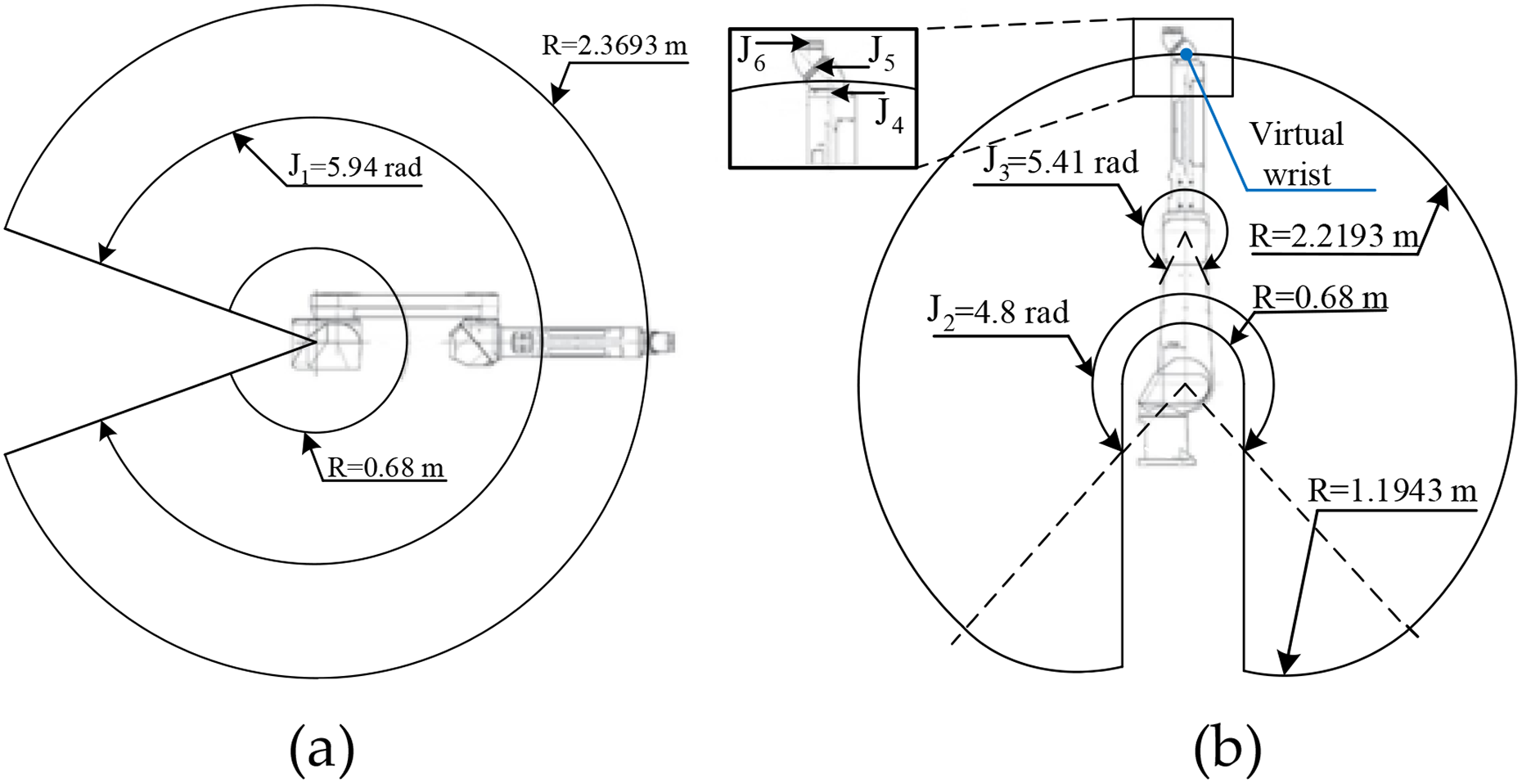
Reachable workspace of TX250 robot. (a) Horizontal section, (b) vertical section.

According to the D-H method, joint coordinates and dimension parameters are defined as shown in Figure 4, and parameter values are listed in Table 1. The transformation matrix between the adjacent two joint coordinates can be expressed as

\begin{matrix} {}_{i}^{i - 1}Τ = Rot (X, α_{i - 1}) Trans(X, a_{i-1}) Rot(Z, θ_{i}) Trans(Z, d_{i}) \\ = [\begin{matrix} c θ_{i} & - s θ_{i} & 0 & a_{i - 1} \\ s θ_{i} c α_{i - 1} & c θ_{i} c α_{i - 1} & - s α_{i - 1} & - d_{i} s α_{i - 1} \\ s θ_{i} s α_{i - 1} & c θ_{i} s α_{i - 1} & c α_{i - 1} & d_{i} c α_{i - 1} \\ 0 & 0 & 0 & 1 \end{matrix}] \end{matrix}

Figure 4.

Coordinate systems and D-H parameters of the TX250 industrial robot.

Table 1.

Parameter values of the TX250 industrial robot.

i	a_i−1 (m)	α_i−1 (rad)	θ_i (rad)	d_i (m)
1	a₀ = 0	α₀ = 0	θ ₁	d₁ = 0.15
2	a₁ = 0.15	α₁ = −π/2	θ ₂	d₂ = 0
3	a₂ = 1.025	α₂ = 0	θ ₃	d₃ = 0
4	a₃ = 0	α₃ = −π/2	θ ₄	d₄ = 1.1943
5	a₄ = 0	α₄ = π/4	θ ₅	d₅ = 0.1247
6	a₅ = 0	α₅ = −π/4	θ ₆	d₆ = 0.0927

And, transformation matrices of the industrial robot, such as ${}_{1}^{0}T$ , ${}_{2}^{1}T$ , ${}_{3}^{2}T$ , ${}_{4}^{3}T$ , ${}_{5}^{4}T$ , and ${}_{6}^{5}T$ , can be calculated sequentially. The entire transformation matrix of the robot terminal relative to the base is the product of above matrices and can be written as

{}^{0}T_{6} = {}^{0}T_{1} {}^{1}T_{2} {}^{2}T_{3} {}^{3}T_{4} {}^{4}T_{5} {}^{5}T_{6}

Equation (2) is the forward position and posture equation for the industrial robot. When the rotation angle of each joint is given, the terminal position and posture of the industrial robot can be determined.

Assume that kinematic parameters of the robot base are ${}^{0}w_{0} = {[\begin{matrix} 0 & 0 & 0 \end{matrix}]}^{T}$ , ${}^{0}{\dot{w}}_{0} = {[\begin{matrix} 0 & 0 & 0 \end{matrix}]}^{T}$ , and ${}^{0}{\dot{v}}_{0} = {[0, 0, - g]}^{T}$ . When the joint angular velocities and accelerations are given, translational velocities and accelerations of points in each link can be deduced in the order from the base to the terminal, with deduced transformation matrices. Centroid velocity and acceleration of each link are solved in the forward direction as ( $i = 0, 1, ..., 5$ )

w_{i + 1} = {}_{i}^{i + 1}R w_{i} + {\dot{θ}}_{i + 1} Z_{i + 1}

{\dot{v}}_{i + 1} = {}_{i}^{i + 1}R ({\dot{ω}}_{i} \times {}^{i}e_{i + 1} + ω_{i} \times (ω_{i} \times {}^{i}e_{i + 1}) + {\dot{ν}}_{i})

{\dot{w}}_{i + 1} = {}_{i}^{i + 1}R {\dot{w}}_{i} + {}_{i}^{i + 1}R w_{i} \times {\dot{θ}}_{i + 1} Z_{i + 1} + {\ddot{θ}}_{i + 1} Z_{i + 1}

{\dot{v}}_{C i + 1} = {\dot{ω}}_{i + 1} \times e_{C i + 1} + ω_{i + 1} \times (ω_{i + 1} \times e_{C i + 1}) + {\dot{v}}_{i + 1}

Symbols w _i, ${\dot{w}}_{i}$ , and ${\dot{v}}_{i}$ are angular velocity, angular acceleration, and linear acceleration vectors of coordinate system i. ${\dot{v}}_{C i}$ is the centroid linear acceleration vector of link i; and ${}_{i}^{i + 1}R$ is the rotation matrix between coordinate systems i + 1 and i, top left section of ${}_{i}^{i + 1}T$ . Z _i is the Z-axis unit vector of coordinate system i. ${}^{i}e_{i + 1}$ is the origin position vector of coordinate system i + 1 in coordinate system i and $e_{C i}$ is the centroid position vector of component i (detailed parameters are presented in Appendix 1).

Inverse kinematics

Inverse kinematics calculation of industrial robot can be decomposed into two steps, such as the initial body position and posture analysis and iterative calculation of the inverse kinematics. As mentioned earlier, there are multiple inverse kinematic solutions for the 6R industrial robot. The initial body position and posture of the robot should be determined first in order to avoid collisions between robot and workpiece during the entire trajectory, which also lays the foundation for the local iterative solution.

Initial body position and posture analysis

The orientation mechanism of the industrial robot is flexible and small in size, which mainly determines the terminal posture and has little influence on the robot body pose. The positioning mechanism is composed of first three joints and directly determines the robot position. Multiple inverse kinematic solutions caused by joints 2 and 3 are analyzed below.

Initial body position and posture analysis shows angle ranges of joints 2 and 3 for each set of inverse kinematic solutions. After the analysis, one set of inverse kinematic solutions will be adopted, and the initial value for iterative calculation can be determined accordingly, which will improve the convergence rate of iterative algorithm and avoid multiple solutions. For the TX250 industrial robot, four sets of inverse kinematic solutions can be deduced and shown in Figure 5. The inverse solution set I is shown with the gray configuration in Figure 5(a), and $θ_{2} \in (- π / 2, 0.83)$ and $θ_{3} \in (0, 1.13)$ . The inverse solution set II is illustrated with the red configuration in Figure 5(a), and $θ_{2} \in (- π / 2, 0.83)$ and $θ_{3} \in (- 4.28, 0)$ . The inverse solution set III is the gray configuration of Figure 5(b), and $θ_{2} \in (- 3.97, - π / 2)$ and $θ_{3} \in (- 4.28, 0)$ . The inverse solution set IV is the red configuration in Figure 5(b), and $θ_{2} \in (- 3.97, - π / 2)$ and $θ_{3} \in (0, 1.13)$ . The inverse solution set I is adopted in the later discussion.

Figure 5.

Inverse kinematic solution sets of positioning mechanism. (a) Inverse solution set I, II; (b) inverse solution set III, IV.

Iterative calculation of inverse kinematics

The TX250 industrial robot is non-orthogonal and the inverse kinematics cannot solve analytically, which is converted to the optimization solution based on the deduced forward pose expressions of equations (1) and (2). The minimum difference between the terminal position and posture that expressed with joint rotation angles and the target terminal position and posture is taken as the optimization goal.

Transformation matrix of the industrial robot ${}^{0}T_{6}$ can be represented as

{}^{0}T_{6} = [\begin{matrix} r_{11} & r_{12} & r_{13} & r_{14} \\ r_{21} & r_{22} & r_{23} & r_{24} \\ r_{31} & r_{32} & r_{33} & r_{34} \\ 0 & 0 & 0 & 1 \end{matrix}]

Accordingly, the terminal position and posture can be expressed as the function of joint angles θ_i as $f (θ_{1}, θ_{2}, θ_{3}, θ_{4}, θ_{5}, θ_{6}) = {[\begin{matrix} r_{14} & r_{24} & r_{34} & r_{13} & r_{23} & r_{33} \end{matrix}]}^{T}$ . The target terminal position and posture is described as $P = {[\begin{matrix} x & y & z & n_{X} & n_{Y} & n_{Z} \end{matrix}]}^{T}$ . x, y, and z represent the terminal position coordinates in the base coordinate system, while n_X, n_Y, and n_Z are the cosine values of angles between the robot terminal and three base coordinate axes. And, the minimum of the two norm is used as the optimization target:

min ‖ f (θ) - P ‖

Based on the optimization model, the PSO algorithm is applied to search the inverse position and posture solutions that meet the specified error requirements (the error adopted here is 10⁻⁶). Initial body position and posture is selected as illustrated in “Initial body position and posture analysis” section and initial joint angles are determined accordingly.

The position and posture relation of the industrial robot established above can be expressed as

f (θ) = P

The velocity mapping between the joint space and the operation space can be obtained by taking the derivative of equation (2) with respect to time, that is

\dot{θ} = J^{- 1} V

where $\dot{θ}$ is the angular velocity vector of robot joints, V is the terminal speed vector, and J ⁻¹ is the inverse matrix of the Jacobian matrix. And the Jacobian matrix can be deduced as $(i \in [1, 2, 3, 4, 5, 6])$ :

J = \frac{\partial f (θ)}{\partial θ_{i}} = [\begin{matrix} J_{11} & J_{12} & J_{13} & J_{14} & J_{15} & J_{16} \\ J_{21} & J_{22} & J_{23} & J_{24} & J_{25} & J_{26} \\ J_{31} & J_{32} & J_{33} & J_{34} & J_{35} & J_{36} \\ J_{41} & J_{42} & J_{43} & J_{44} & J_{45} & J_{46} \\ J_{51} & J_{52} & J_{53} & J_{54} & J_{55} & J_{56} \\ J_{61} & J_{62} & J_{63} & J_{64} & J_{65} & J_{66} \end{matrix}]

By taking the derivative of equation (10) with respect to time, we can obtain mapping equation between the joint acceleration and the terminal motion state, which can be expressed as

\ddot{θ} = J^{- 1} [\dot{V} - {(J^{- 1} V)}^{T} H (J^{- 1} V)]

where $\dot{V}$ is the terminal acceleration vector, and H is the Hessian matrix, which can be obtained by solving the derivative of the Jacobian matrix about joint angles.

Dynamic modeling and simulation

In this section, the Newton–Euler method is adopted to deduce the dynamic model of the industrial robot, in order to analyze the reaction force and torque of the robot acting on the flexible supported teleplatform. Based on deduced kinematics, joint angles are determined with the iterative calculation of equation (8). Then, joint angular velocities and accelerations are figured out with the inverse kinematics of equations (10) and (12). Finally, velocities and accelerations of each robot link are deduced with forward kinematics of equations (3) to (6), which is the basis of the dynamic modeling.

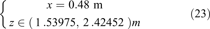
Since the external force and torque exerted to the robot terminal are known, the force and torque of each joint can be solved following the order that from the terminal to the base. Specifically inertial force, joint force, inertial torque, and driving torque of each link are expressed as $(i = 5, 4, 3, 2, 1)$

F_{C i +1} = m_{i + 1} {\dot{v}}_{C i + 1}

f_{i} = {}_{i + 1}^{i}R f_{i + 1} + F_{C i}

N_{C i + 1} = I_{C i + 1} {\dot{w}}_{i + 1} + w_{i + 1} \times I_{C i + 1} w_{i + 1}

n_{i} = N_{C i} + {}_{i + 1}^{i}R n_{i + 1} + e_{C i} \times F_{C i} + {}^{i}e_{i + 1} \times {}_{i + 1}^{i}R f_{i + 1}

τ_{i} = n_{i}^{T} Z_{i}

where f _i and n _i are force and torque vectors that the link i − 1 acts on the link i in coordinate system i; $I_{C i}$ is the inertial matrix of the link i relative to the mass center in coordinate system i (unit: kg ⋅ m); $F_{C i}$ and $N_{C i}$ : inertia force and torque of link i about the mass center.

The reaction force and torque that the industrial robot exerted on the flexible supported teleplatform are solved according to the force and torque of the robot base and can be expressed as

F_{0} = {}_{1}^{0}R f_{1} + F_{C 1}

T_{0} = N_{C 0} + {}_{1}^{0}R n_{1} + e_{C 0} \times F_{C 0} + {}^{0}e_{1} \times {}_{1}^{0}R f_{1}

There are no external force or torque for the spraying robot, and $f_{6} = {[\begin{matrix} 0 & 0 & 0 \end{matrix}]}^{T}$ and $n_{6} = {[\begin{matrix} 0 & 0 & 0 \end{matrix}]}^{T}$ .

In order to verify the established dynamic model, simulation comparison between the deduced dynamics model and the ADAMS software is carried out. The terminal trajectory is given as

{\begin{matrix} x = \sqrt{1.175} (1 - \frac{3}{2 T^{2}} t^{2} + \frac{1}{T^{3}} t^{3}) \\ y = \sqrt{1.175} (\frac{3 \sqrt{3}}{2 T^{2}} t^{2} - \frac{2 \sqrt{3}}{2 T^{3}} t^{3}) \\ z = - 0.8252 \\ n_{X} = 0; n_{Y} = 0; n_{Z} = - 1 \end{matrix}

where the total time is 1 s (T = 1 s), $[0, - 0.1, 0.2, 0, 0, 0]$ is the initial joint angle deduced with the initial body position and posture analysis (dynamic parameters are presented in Appendix 1).

Joint driving torques are shown in Figure 6, while the reaction force and torque that robot exerted on the flexible supported teleplatform is illustrated in Figure 7. Figures indicate that the calculation result with the deduced dynamic model is consistent with the ADAMS [2015 version] simulation results, and the correctness of the established dynamic model is well verified.

Figure 6.

Joint driving torques.

Figure 7.

Reaction force and torque.

Analysis of body accuracy

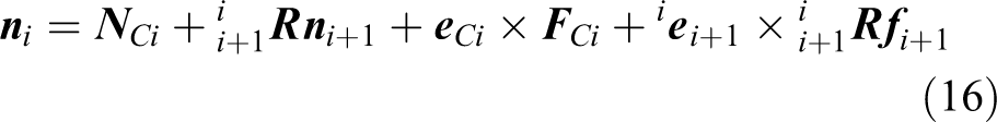
The first three joints are in the form of rotating joint-driven pendulum. The joint rotation error will be amplified, and the position accuracy is difficult to guarantee. The last three joints are mainly used to achieve posture, whereas accuracy depends directly on the accuracy of joints. Thus, body accuracy mainly refers to the position precision analysis of the industrial robot in the workspace and is determined by the first three joints. The LCI is used to analyze the precision. The condition number of the Jacobian matrix can be expressed as

K = \frac{σ_{max}}{σ_{min}}

where σ_max and σ_min are maximum and minimum singular values of the Jacobian matrix, and 1 ≤ K < ∞. The LCI of the robot is defined as the reciprocal of the Jacobian matrix condition number, that is, Γ = 1/K. When the value of LCI is large, the robot terminal has good position accuracy. Otherwise, the accuracy of the robot terminal is poor.

According to the previous analysis, joints 2 and 3 determine the boundary of the reachable workspace in the XOZ plane for the 6R industrial robot. Then, the entire reachable workspace of the robot is formed with the rotation of joint 1. Therefore, distribution analysis of the LCI value is carried out on the XOZ section of the reachable workspace, as shown in Figure 8. Considering potential interference between the motion platform and the TX250 robot, lower part of the reachable workspace is not included in the analysis. The initial body position and posture used in this analysis is the same as the gray link pose in Figure 5(a), which is in the range of $θ_{2} \in (- π / 2, 0.83)$ and $θ_{3} \in (0, 1.13)$ .

Figure 8.

LCI distribution on XOZ plane. LCI: local conditioning index.

From Figure 8, we can see that the LCI value increases first and then decreases as the terminal moves from the outer boundary to the base. The minimal LCI value appears around the outer boundary, and the minimum LCI value is located at the top left corner with small X value and large Z value. Generally, when the robot terminal moves near the outer boundary of the workspace, the accuracy of the robot body is poor.

Reaction ellipsoid indices and workspace analysis

For the flexible supported industrial robot, the motion of the robot will produce reaction force and torque on the flexible supported teleplatform, which could cause vibration of the flexible supported teleplatform and deterioration of the terminal accuracy. At present, the driving and control modules of the industrial robot are highly solidified. The vibration suppression control methods, such as input filtering, are difficult to implement. Interruptions of the spraying operation as a cost of internal force vibration suppression are not allowed. In this section, reaction force and torque exerted on the flexible supported teleplatform, which are mainly caused by the acceleration of the robot, is investigated. By controlling reaction force and torque within the reasonable ranges, excessive vibration and terminal error are avoided, thus presenting a practical engineering solution to suppress vibration and improve terminal accuracy.

Posture mechanism of the industrial robot is small with lightweight and has little contribution to the reaction force and torque, which is also illustrated in the dynamic simulation result of joints 4 to 6 in “Dynamic modeling and simulation” section. In this section, joints 1, 2, and 3 are mainly considered to establish the reaction force and torque ellipsoids under the terminal unit acceleration requirement. Lengths of long axes of the reaction force and torque ellipsoids are considered as evaluation indices of reaction force and torque exerted to the flexible supported teleplatform. The high-quality workspace is decided by the LCI of last section and reaction ellipsoid indices together.

Reaction ellipsoid indices

The terminal position of the industrial robot is expressed as $P = {[\begin{matrix} x & y & z \end{matrix}]}^{T}$ , while the terminal acceleration unit vector is $\dot{V} = {[\begin{matrix} \ddot{x} & \ddot{y} & \ddot{z} \end{matrix}]}^{T}$ . The reaction force that exerted on the flexible supported teleplatform is $F_{0} = {[\begin{matrix} F_{0X} & F_{0Y} & F_{0Z} \end{matrix}]}^{T}$ . Then, the mapping between reaction force and terminal unit acceleration can be illustrated as

F_{0} = A \dot{V}

Matrix A can be determined based on the previously established dynamics model. With the singular-value decomposition, eigenvalues and eigenvectors of matrix A can be deduced, which determine length and direction of each axis of the reaction force ellipsoid. The length of the longest axis is considered as the reaction force ellipsoid index. The value distribution of this index in the XOZ section of the reachable workspace is obtained and shown in Figure 9. The index values range from 70 N to 120 N, and the maximum value appears in the upper left corner. Generally, as the robot terminal moves from the outer boundary to the base, the index value decreases and then increases, and the index value of the inner boundary near the base is large.

Figure 9.

Value distribution of reaction force ellipsoid index.

Similarly, the reaction torque ellipsoid of the robot can be obtained by establishing the mapping relationship between the reaction torque and the terminal unit acceleration. The length of the longest axis is the reaction torque ellipsoid index. The value distribution of this index can be determined and shown in Figure 10. The torque ellipsoid index values range from 70 Nm to 200 Nm. The maximum value also appears in the upper left corner, and the minimum value lies in the lower part. The overall value distribution of the torque index is similar to that of the reaction force ellipsoid index. When the robot moves near the boundary, the reaction force and torque are larger and cause greater vibration with worse terminal accuracy.

Figure 10.

Value distribution of reaction torque ellipsoid index.

High-quality workspace

According to the actual accuracy requirements of the industrial robot, value ranges of LCI and reaction spherical indices can be determined. In the follow-up analysis, constraints are given as follows: LCI value ≥2.5, value of the reaction force ellipsoid index ≤90 N, and value of the reaction torque index ≤120 Nm. Above requirements are illustrated in the XOZ section of reachable workspace and shown in Figure 11.

Figure 11.

Boundaries of LCI and reaction ellipsoid indices. LCI: local conditioning index.

In the figure, the Fw curve illustrates the flexible workspace boundary, the Fe curve shows the boundary of the reaction force ellipsoid index, the Te curve is the boundary of the reaction torque ellipsoid index, and the Aw curve is the reachable workspace boundary. Intersection of above available areas is the high-quality workspace that meets the terminal accuracy requirements.

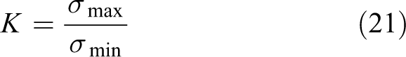
Boundary of the high-quality workspace shown in Figure 11 is irregular and difficult to describe in algebra, which is not conducive to the analysis of robot station and trajectory plan. The regularized high-quality workspace is the interior space between concentric spheres and becomes a ring in the XOZ section, as shown in Figure 12. The center is located at (0, 0, 0.55) m, and inside and outside radius are 1.1 m and 1.935 m, respectively. Besides, the upper and lower boundary can be expressed as cylinder and cone. The expressions of the upper and lower boundaries in the XOZ section can be respectively expressed as

{\begin{matrix} x = 0.48 m \\ z \in (1.53975, 2.42452) m \end{matrix}

{\begin{matrix} z = 7 x - 6.2 \\ x \in (0. 706967, 0. 867702) m \end{matrix}

Figure 12.

Boundaries of regularized high-quality workspace.

The regularized high-quality workspace of the industrial robot can be established as shown in Figure 13.

Figure 13.

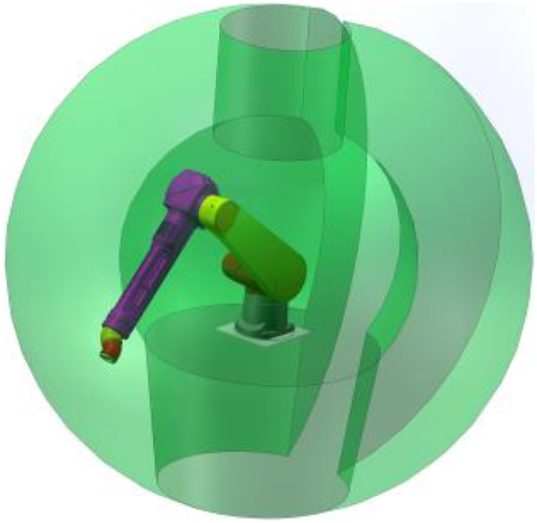
Regularized high-quality workspace.

Simulations

The numerical simulation is used to verify the effectiveness of the deduced high-quality workspace in terms of limiting the reaction force and torque acting on the flexible supported teleplatform during the motion of industrial robot. As shown in Figure 14, there are eight straight lines and five points evenly distributed on each line in the XOZ section of the reachable workspace (point locations are listed in Appendix 2). For each line, points 1 and 5 are outside the regularized high-quality workspace, while points 2, 3, and 4 are inside it. The terminal of the industrial robot is located at each point with the acceleration of 2 m/s² along three coordinate axes of the base coordinate system. Reaction force and the torque exerted on the flexible supported teleplatform corresponding to each point are organized and shown in Figures 15 and 16.

Figure 14.

Locations of lines and points.

Figure 15.

Simulation results of reaction force.

Figure 16.

Simulation results of reaction torque.

In Figure 15, reaction forces at points 1 and 5 on each line are larger than those at points 2, 3, and 4 and reflect the inhibitory effect of the high-quality workspace on limiting the amplitude of the reaction force. In addition, the reaction force of point 1 is greater than that of point 5, which is in accordance with the value distribution of the reaction force ellipsoid index in Figure 9. The mean of reaction forces of points in the regularized high-quality workspace is 119.0278 N, which is only 49.54% of the average value of reaction force of points outside the workspace.

Figure 16 illustrate that the reaction torques at points 1 and 5 are greater than the reaction torques generated at points 2, 3, and 4, which reflects the effect of high-quality workspace on reducing reaction torque. The average reaction torque of points within the regularized high-quality work space is 136.6002 Nm, which is only 48.02% of the average value of points outside the workspace.

Conclusions

Terminal precision of the flexible supported industrial robot was investigated in this study. The reachable workspace for the industrial robot was established based on the virtual wrist. The position accuracy of the robot was analyzed with the LCI. Simulation results showed that as the robot terminal moved from the outer boundary of the reachable workspace to the base, the LCI value increased and then decreased, and the minimal LCI values appear near the outer boundary.

The reaction force and torque ellipsoids are proposed on the basis of the terminal unit acceleration. Lengths of ellipsoid long axes were adopted as indices to evaluate the reaction force and torque that the industrial robot exerted on the flexible supported teleplatform. Value distributions of reaction force and torque ellipsoid indices in the workspace were analyzed. As the robot terminal moved from the outer boundary of the workspace to the base, index values decreased and then increased, and larger values appears on the inner boundary. Finally, a high-quality workspace was established, considering the comprehensive requirements of LCI and reaction ellipsoid indices.

The effectiveness of the high-quality workspace is validated through numerical simulation. Results showed that the average reaction force of points in the regularized high-quality workspace was 119.0278 N, which was only 49.54% of that of points outside the workspace. The mean of reaction torques of points in the regularized high-quality workspace was 136.6002 Nm, which was only 48.02% of that of points outside the workspace. The proposed method avoids modifications of the robot control system, ensures motion continuity, and provides a practical solution to improve the terminal accuracy of the flexible supported industrial robot.

Footnotes

Declaration of conflicting interests

The authors declared no potential conflicts of interest with respect to the research, authorship, and/or publication of this article.

Funding

The authors disclosed receipt of following financial support for the research, authorship, and/or publication of this article: This research is jointly sponsored by the National Natural Science Foundation of China (No. 51575292), National Science and Technology Major Project of China (No. 2016ZX04004004), and National Intelligent Manufacturing Project of China (Application of intelligent manufacturing new mode on a new generation of high-efficiency photovoltaic cell).

ORCID iD

Lian Chen

Zhufeng Shao

Appendix 1

Kinematic and dynamic parameters of the Staubli TX250 industrial robot.

1. Mass of each link (kg):

Appendix 2

Table 2H.

Point locations and simulation results of line 8.

_Point	_{Force (N)}	_{Torque (Nm)}	_{Coordinate (m)}
1	291	313	(0.723, 0, −0.713)
2	77	63	(0.941, 0, −0.611)
3	116	69	(1.262, 0, −0.462)
4	148	93	(1.641, 0, −0.285)
5	205	167	(2.110, 0, −0.066)

References

Shao

Tang

Wang

. Dynamic modeling and wind vibration control of the feed support system in fast. Nonlinear Dynamics 2012; 67(2): 965–985.

Zhao

. The development status and challenge of industrial robots in China. Aero Manufact Technol 2012; (12): 27–29.

Shao

Tang

Wang

. A fuzzy PID approach for the vibration control of the FSPM. Int J Adv Robot Sys 2013; 10(59): 1–8.

NIST RoboCrane® Cuts Aircraft Maintenance Costs. https://www.nist.gov/news-events/news/2007/07/nist-robocrane%C2%AE-cuts-aircraft-maintenance-costs (2010, accessed 31 July 2018).

Liu

Chen

Shao

. Research on terminal accuracy guarantee of FAST feed support system. J Mech Eng 2017; 53(17): 50–59.

Yuan

. Workspace analysis of cable-driven continuum manipulators based on static model. Robot Comp Int Manuf 2018; 49: 240–252.

Ren

Omisore

Han

. A Master-Slave control system with workspaces isomerism for teleoperation of a snake robot. In: 2017 39th annual international conference of the IEEE engineering in medicine and biology society (EMBC), 11–15 July 2017, Seogwipo, South Korea, pp. 4343–4346. IEEE.

Heo

Choi

Park

. Workspace analysis of a 6-DOF cable-driven parallel robot considering pulley bearing friction under ultra-high acceleration. Microsyst Technol 2017; 23(7): 2615–2627.

Ryu

. A multi-subband Monte Carlo study on dominance of scattering mechanisms over carrier transport in sub-10-nm Si nanowire FETs. Nanoscale Res Lett 2016; 11(1): 36.

10.

Choi

Park

Kim

. A manipulator workspace generation algorithm using a singular value decomposition. In: International conference on control automation and systems, Seoul, South Korea, 14–17 October 2008, pp. 163–168. IEEE.

11.

Sauvet

Laliberte

Gosselin

. Design, analysis and experimental validation of an ungrounded haptic interface using a piezoelectric actuator. Mechatronics 2017; 45: 100–109.

12.

Goyal

Sethi

. An analytical method to find workspace of a robotic manipulator. J Mech Eng 2010; 41(1): 25–30.

13.

Kwon

Youm

. General algorithm for automatic generation of the workspace for n-link redundant manipulators. In: International conference on advanced robotics 1994, Pisa, Italy, 19–22 June 1991, pp. 1722–1725. New York, NY: IEEE.

14.

Yang

Miao

. Inverse kinematics of a class of 7R 6-DOF robots with non-spherical wrist. In: International conference on mechatronics and automation 2013, Takamatsu, Japan, 4–7 August 2013, pp. 69–74. New York, NY: IEEE.

15.

Azad

Babič

Mistry

. Dynamic manipulability of the center of mass. A tool to study, analyse and measure physical ability of robots. In: 2017 IEEE international conference on robotics and automation (ICRA), 29 May–3 June 2017, Singapore, pp. 3484–3490. IEEE.

16.

Zhang

Liang

Wang

. Manipulability measure of a dual-arm space robot and its application to configuration optimization. J Astronaut 2016; 128: 322–329.

17.

Khan

Angeles

. The kinetostatic optimization of robotic manipulators. J Mech Des 2006; 128(1): 168–178.

18.

Merlet

. Jacobian, manipulability, condition number and accuracy of parallel robots. J Mech Des 2006; 128(1): 199–206.

19.

Gosselin

. Determination of the workspace of 6-DOF parallel manipulators. J Mech Des 1990; 112(3): 331–336.

20.

Primrose

EJF

. On the input-output equation of the general 7R-mechanism. Mech Mach Theory 1986; 21(6): 509–510.

21.

Wang

Yang

Zhang

. An inverse kinematics algorithm of the general 6-DOF robot based on Newton-Raphson iteration. Trans Microsyst Technol 2010; 178(178): 123–131.

22.

Kennedy

Eberhart

. Particle swarm optimization. In: IEEE international conference on neural networks, Perth, Australia, 27 December 1995, pp. 1942–1948. IEEE.

23.

Tang

Shao

. Trajectory planning and tracking control of a multi-level hybrid support manipulator in FAST. Mechatronics 2013; 23(8): 1113–1122.

24.

Sciavicco

Siciliano

Villani

. Lagrange and Newton-Euler dynamic modeling of a gear-driven robot manipulator with inclusion of motor inertia effects. Adv Robot 1995; 10(3): 317–334.

25.

Miller

Clavel

. The Lagrange-based model of Delta-4 robot dynamics. Robotersysteme 1992; 8: 49–54.

26.

Hao

Guan

Wang

. Dynamic feedforward control of the 2-DOFs parallel manipulator of a hybrid machine tool. In: 8th IEEE International Conference on Control and Automation (ICCA 2010), Xiamen, China, 9–11 June 2010, pp. 528–533. IEEE.

27.

Wang

. Motion control of the 2-DOF parallel manipulator of a hybrid machine tool. Robotica 2010; 28(6): 861–868.

28.

https://www.ctisystems.com/references/aviation-teleplatforms/teleplatform-cranes-airbus/ (accessed 31 July 2018).

29.

https://en.wikipedia.org/wiki/St%C3%A4ubli (accessed 31 July 2018).

Analysis of flexible supported industrial robot on terminal accuracy

Abstract

Keywords

Introduction

Workspace and forward kinematics

Inverse kinematics

Initial body position and posture analysis

Iterative calculation of inverse kinematics

Dynamic modeling and simulation

Analysis of body accuracy

Reaction ellipsoid indices and workspace analysis

Reaction ellipsoid indices

High-quality workspace

Simulations

Conclusions

Footnotes

Declaration of conflicting interests

Funding

ORCID iD

Appendix 1

Appendix 2

References