Sage Journals: Discover world-class research

Abstract

This article proposes a collision detection algorithm without external sensors that can detect potential collisions in man–robot interaction. The algorithm is based on a modified first-order momentum deviation observer that also takes friction into account. The collision detection algorithm uses joint angles, angular velocities, and torques during the detection process, without any need to consider angular acceleration. The algorithm also uses an accurate friction model that is based on a Stribeck model with second-order Fourier series compensation. The friction model is applied in advance so that compensation can be made in real time during collision detection. Identification data are filtered through a first-order low-pass filter to reduce high-frequency noise. In order to verify the algorithm, a simulation and experiment were carried out using a collaborative robot experimental platform. The results confirmed that collisions can be detected by setting appropriate threshold values. Different possible responses can be implemented according to different response strategies, with the ultimate arbiter being that collision forces are kept strictly within ordinary human tolerances. This makes sure that safety can be preserved in man–robot interaction processes.

Keywords

Collision detection momentum deviation friction identification external torque observer collaborative robot

Introduction

With industrial robots becoming more popular in the 3C (computer, communication and consumer electronics) industry, collaborative robots with lightweight, flexible movements, and simple controls have great development potential. However, as collaborative robots share the working environment with people, this makes man–robot interaction inevitable, producing a real risk of accidental man–robot contact. As a result, safety is an important feature in man–robot collaboration algorithms.^1,2 Safety controls require that robots have the ability to detect possible collisions and respond, making unexpected collisions less likely.³ This article focuses on collision detection algorithms.

There is a lot of research on collision detection algorithms for collaborative robots, centered on the use of different kinds of external sensors.^4,5 Sensors used to detect collisions include visual sensors,⁶ tactile sensors,⁷ laser sensors,⁸ and different types of torque sensors.^9,10 Detection algorithms using external sensors have a number of advantages, including high sensitivity and precision, but the control algorithms are complex. Detecting where collisions might happen often involves multi-sensor combinations, increasing the complexity of the physical structure, threading difficulties, and ultimately, the cost of the robot. This makes collision detection algorithms hard to apply.

Key to overcoming these issues is the elimination of external sensors. Elastic joint modules can limit collision damage using elastic elements while ensuring angular precision,¹¹ but this has many shortcomings and lacks flexibility. When collision detection algorithms with no external sensors are used, detection is feasible using just observed values calculated using parameters of motion and torque. These can be obtained using internal sensors that collect current values of servo motor and encoder data. The observed values have to meet certain requirements, which are as follows: (1) the value is equal or close to 0 for “no collision”; (2) the value increases very rapidly when collisions occur and with little delay; and (3) the value decays quickly when a collision is terminated. In practice, an appropriate threshold value has to be set. When an observed value exceeds the threshold, a collision is assumed to be happening and a response strategy is implemented. So, detection sensitivity depends on keeping the threshold values to a minimum, which makes it necessary to keep “no collision” observed values as small as possible.

In this regard, making observed values equal to the difference between the torque calculated by the motion parameters and the actual torque has been proposed by Yamada et al.¹² However, this is influenced by acceleration and is hard to apply if the velocities change frequently. A collision detection algorithm based on a disturbance observer was proposed by Haddadin et al. and has been widely applied.¹³ However, angular acceleration obtained by differentiating angular velocity is necessary for this. Another detection algorithm based on energy conservation was established by De Luca et al.,¹⁴ but here accuracy and rapidity are interdependent and cannot be optimal at the same time.

When angular acceleration is obtained using differentials, the data has a lot of noise and delay. This has recently led to the development of detection algorithms based on generalized deviation of momentum instead of angular acceleration, resulting in greater stability. Relevant research here includes the first-order algorithm proposed by De Luca et al.,¹⁵ which has excellent responsivity and accuracy, and the second-order algorithm proposed by He et al. that has more adjustable parameters.¹⁶ This improves the filtering but makes the parameter adjustment more complex. D’Ippolito et al. compared the momentum-based method and an error-based method and proposed a reaction control law to reduce the impact of a collision.¹⁷ Meanwhile, the first-order detection algorithm has been modified by Cho et al. to enable differentiation between intended contact and unexpected collision, using the rate of change of observed values.¹⁸ The second-order detection algorithm was modified to allow for the import of an adjustment function that can improve the performance of the observer tracking for the external torque.

However, none of the above-mentioned algorithms consider friction torque. As a result, observed values depend on superimposed torques for friction and collision, which means that the threshold value cannot be set universally and has to be adjusted for different working processes. Some research regarding collision detection in recent years has incorporated aspects of friction into its algorithms. These algorithms mostly use a simple first-order observer with Coulomb and viscous friction compensation^19
–21 and are able to improve the performance to some extent with better collision detection. However, the adopted friction models do not consider the influence of joint angles. This undermines the detection accuracy for collaborative robots that have large assemblies or that are very heavy.

Another issue here is that detection algorithms based on generalized momentum deviation observers require the development of dynamic models. Traditional calculations of observed values do not consider how internal rotating components will impact on the inertia tensor of the joints. However, compensation for inertial forces is essential.

In this article, we present a collision detection algorithm that takes joint friction into account without using external sensors. The algorithm is based on a first-order momentum deviation observer and the need to low-pass filter data in advance. Identification of the friction model is carried out beforehand, and compensation for friction is processed in real time. The friction model is Stribeck model with second-order Fourier series compensation and is suitable when robot joints run at either low or high speeds. To verify the validity of the algorithm, we conducted an experiment using a lightweight modular lab-designed collaborative robot. The results show that the algorithm can accurately calculate observed values, with an observed value close to 0 for “no collision,” and a value approximately equal to the external torque when a collision occurs, making collaborative robot collision detection possible for any position.

External torque observer

Design of the external torque observer

The momentum deviation observer can be applied to the identification of friction torques as well. When a collaborative robot has a collision with its external surroundings, there will be torque affecting the joints in front of the collision point because of the collision force. This means that the dynamic equation for a robot with n degrees of freedom (DOFs) can be expressed as

M (q) \ddot{q} + C (q, \dot{q}) \dot{q} + G (q) + τ_{f} = τ_{d} - τ_{c}

where q , $\dot{q}$ , and $\ddot{q}$ are vectors with n × 1 of joint angles, angular velocities, and angular acceleration. M ( q ) is the inertia matrix for the robot. $C (q, \dot{q})$ is the matrix containing Coriolis and centrifugal terms, and G ( q ) is the gravity vector. τ _f is the joint friction torque vector produced by transmission; τ _d is the joint driving torque, which is approximately equal to the product of the motor torque and the reduction ratio; and τ _c is the joint collision torque produced by an external collision force, which can be calculated thus

τ_{c} = J^{T} F_{c}

where J is the Jacobian matrix, and F_c is the collision force.

There are many ways to build the dynamic model in equation (1). In order to express the model explicitly, a dynamic model can be built using a Lagrangian equation.²² Figure 1 provides a three-dimensional (3-D) model of the target robot, which is a kind of 6 Rotational-joints (6R) nonorthogonal modular collaborative robot.

Figure 1.

3-D model of the experimental robot. 3-D: three-dimensional.

In order to make the processing of the torque more straightforward, an external torque vector τ _e was defined. This includes the joint friction torque and the equivalent torque for collision force when transmitted by a harmonic reducer. So

τ_{e} = τ_{c} + τ_{f}

Combined with equation (1), the external torque can now be expressed as

τ_{e} = τ_{d} - (M (q) \ddot{q} + C (q, \dot{q}) \dot{q} + G (q))

In order to solve equation (4), while avoiding noise in the process of collecting robot angular acceleration $\ddot{q}$ at the same time, an external torque observer was designed based on the principle of the conservation of generalized momentum.

The conservation of generalized momentum for a robot can be expressed by

p = M (q) \dot{q}

where p is the generalized momentum of the robot, M ( q ) is a positive symmetric matrix, and $\dot{M} (q) - 2 C (q, \dot{q})$ is an antisymmetric matrix.²³ $\dot{M} (q)$ can therefore be expressed as

\dot{M} (q) = C^{T} (q, \dot{q}) + C (q, \dot{q})

Combining equations (4), (5), and (6), the time derivative of p can be expressed by

\dot{p} = τ_{d} - τ_{e} + C^{T} (q, \dot{q}) \dot{q} - G (q)

In order to estimate the external torque τ _e, the vector r by n × 1 is defined as

r = K_{r} (\hat{p} - p)

where K _r is the gain matrix of the external torque observer, and $\hat{p}$ is the estimated value of p . Combined with equation (7), $\hat{p}$ can be expressed by

\dot{\hat{p}} = τ_{d} - r + C^{T} (q, \dot{q}) \dot{q} - G (q)

Integrated with time on both sides of equation (9), the model can be combined with equation (8) and rewritten as

r (t) = K_{r} {\int_{0}^{t} [τ_{d} + C^{T} (q, \dot{q}) \dot{q} - G (q) - r] - p}

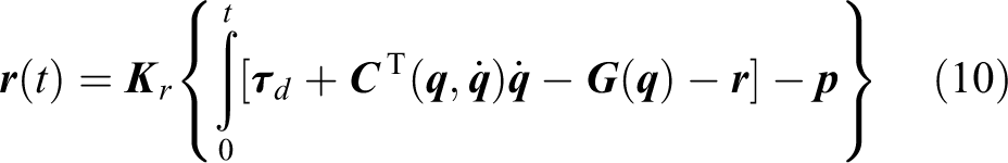
The external torque observer shown in equation (10) is the criterion used to judge whether a collision has taken place or not. The observer only requires the collection of angles, angular velocities, and torques of joints. There is no need to calculate joint angular acceleration.

Algorithmic optimization

If we take the derivative with respect to time on both sides of equation (8), it can be combined with equations (7) and (9) and rewritten as

\dot{r} = K_{r} (- r + τ_{e})

Using a Laplace transformation on both sides gives

\frac{r (s)}{τ_{e} (s)} = \frac{K_{r}}{K_{r} + s}

As shown in equation (12), when K _r → ∞, if there is no collision, the observer r converges to τ _f according to the exponent rule. If a collision occurs, r converges to τ _e. This gives the algorithm two directions: the identification of friction torques and the assessment of collision torques after friction compensation.

The observer also works as a kind of first-order low-pass filter, so an appropriate gain value has to be designed to improve responsivity and ensure robustness.

The collision algorithm being first order, there is just one adjustable parameter. This makes it difficult to provide both accuracy and speed at the same time. A proportional element is therefore introduced: the gain K. The transfer function now reads as

\frac{r (s)}{τ_{e} (s)} = \frac{K_{d}}{K_{r} + s}

where K_d = KK_r.

Identifying friction in the joint

Building the friction model

Harmonic reducers are widely used in various kinds of robots because they have no gear teeth flank interval and can reach high load/weight ratios. Most robot joints therefore use a combination of servo motors and harmonic reducers. There is a lot of research on modeling and identifying friction. Many models have been proposed, for example, the Coulomb and viscous friction model,⁵ the LuGre friction model,²⁴ the Stribeck friction model,²⁵ the cubic polynomial model, and the generalized maxwell slip (GMS) model.^26,27 Torque can be identified by obtaining data from a joint torque sensor or calculated using a dynamic model. Here, however, we present a novel method of identification which uses an external torque observer that does not change a robot’s physical structure or import any differential noise.

The modified Coulomb and viscous friction model adopted by Lee and Song¹⁹ is the one that is most often used in man–robot interaction control. It divides friction compensation into three states: static states, quasi-startup states, and running states. These are distinguished by assessing whether the actual speed and setting speed are 0 or not. The disadvantage of this approach is that the impact of the joint angles on the friction torques is not considered. The form of transmission used by harmonic reducers means their friction depends on both angular velocities and the angles themselves. Friction here includes Coulomb and viscous friction. It also depends on cyclical fluctuations of the joints at low speed. This necessitates additional compensation using a second-order Fourier series. For a collaborative robot running at lower speeds, the Stribeck friction model is better able to capture the negative slope of the friction curve. We have therefore adopted a Stribeck model with second-order Fourier series compensation. The model is composed of two parts. The first relates to joint angles

F_{p} (q) = B_{1} sin q + B_{2} cos q + B_{3} sin (2 q) + B_{4} cos (2 q)

where F_p(q) is the friction torque related to joint angles, q is the joint angles, and B₁, B₂, B₃, B₂ are coefficient gains.

The other part relates to angular velocities

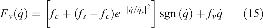
F_{v} (\dot{q}) = [f_{c} + (f_{s} - f_{c}) e^{- | \dot{q} / {\dot{q}}_{s} |^{2}}] sgn (\dot{q}) + f_{v} \dot{q}

where $F_{v} (\dot{q})$ is the friction torque related to angular velocities, f_c is the Coulomb friction force, f_s is the static friction force, $\dot{q}$ is the joint angular velocities, ${\dot{q}}_{s}$ is the Stribeck speed, and f_v is the viscous friction coefficient.

If we combine the two parts, the friction model for a harmonic drive joint can be expressed as

τ_{f} = F_{p} (q) + F_{v} (\dot{q})

where τ_f is the total friction torque of the joint.

Friction needs to be identified and processed for six joints independently. The joints have to run without load and external collision force, and the angles, angular velocities, and joint torques need to be collected. If the rotation axis of the joint is parallel to gravity, joint torque is equal to friction torque. To make the curve fit better in a MATLAB [Version R2015a] environment, the fitting function can be rewritten as

τ_{f} = a \dot{q} + b + c exp (- d {\dot{q}}^{2}) + e sin (q) + f cos (q) + g sin (2 q) + h cos (2 q)

where a, b, c, d, e, f, g, h are the fitting coefficients, τ_f is the friction torque of the joint, $\dot{q}$ is the angular velocity of the current joint, and q is its angle.

Friction identification experiment

Filtering preprocessing

Information such as angles, angular velocities, and joint torques, collected by collaborative robots in real time, contain noise with different frequencies, especially high-frequency noise produced by the sampling process. Some filtering therefore has to be conducted in advance. Commonly used low-pass filters include average filters, Kalman filters,²⁸ and the multi-order filter proposed by Gandhi et al.²⁹ Here, the filtering processing is carried out after collecting the information, rather than after the calculation of observed values, thereby avoiding any cumulative error and providing greater robustness and a lower wrong detection ratio.

Average filters have been proved to have low offset and a simple structure, but their filtering effect is poor. Kalman filters were first proposed for flight guidance and quickly spread to other fields. They obtain a true value by estimating the prior value and observing the current value. These necessitate much less storage capacity, making them suitable for real-time applications. However, high-frequency sampling significantly increases the amount of calculation, and the cumulative error causes data distortion. Multi-order filters work by changing amplitude in the frequency domain. This requires a simple algorithm, has good real-time capability, and produces a value very close to the true value. The structure of the filter model is

Q (s) = \frac{\sum_{k = 0}^{M} α_{k} {(τ s)}^{k}}{{(τ s + 1)}^{N}}

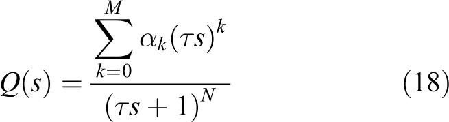
where $α_{k} = \frac{N!}{(N - k)! k!}$ is the binomial coefficient, N is the denominator order, and M is the numerator order. N − M is the relative order, and τ is the filter’s time coefficient.

The trajectory of a robot is set in advance, and the motion parameters and torque information are collected through the drive program of the controller, whose sampling interval is 0.01 s. The torque curve before and after filter processing is shown in Figures 2 and 3, respectively. Increasing the order of the filter reduces stability and affects the observed value. The filter therefore uses a stable first-order filter where the time coefficient is equal to five times the sampling time, that is, 0.05 s. The transfer function is

Q (s) = \frac{1}{0.05 s + 1}

Figure 2.

Joint torque curve before filtering.

Figure 3.

Joint torque curve after filtering.

It can be seen in Figure 3 that the filtering effect is obvious and noise fluctuations are low. As required, the model is close to the true value. Thus, the selected low-pass filter filters the noise effectively and provides a smooth curve. The calculated value after filtering has a data error of under 10%.

Joint friction identification

The torques generated by friction account for a large part of the torque overall, so it is important to identify and compensate for joint friction torque. Friction torque is generated mostly by the secondary reduction transmission in the reducer and contact between the belt and the wheel.

The friction model here relates to the direction of the joint’s angular velocity, so identification has to be carried out twice, on either side of the direction. The following is an example of identification processing for joint 1 in a positive direction. The adopted trajectory used uniform acceleration and deceleration. This made it easier to collect the torque information for different angular velocities and it could be fitted to the friction curve more effectively. A single identification experiment collected 2048 data points; 1212 data points were stored during the joint 1 identification after setting the trajectory, collecting the information, filtering, and taking out the point of greatest deflection. The data points were fitted using the least square method with a MATLAB toolbox. The fitting function adopted the model expressed in equation (17). The results are shown in Figure 4, and the fitting coefficients for all joints are shown in Table 1.

Figure 4.

Fitting curve generated by the novel friction model.

Table 1.

Coefficients of the joint friction model.

Joint	a	b	c	d	e	f	g	h	RMSE
1(+)	144.2648	−130.321	134.1	0.6634	1.237	−0.685	1.236	1.516	4.8807
1(−)	122.7848	136.8963	−107.6	0.5817	−1.535	−15.92	1.908	9.705	6.1725
2(+)	152.7403	−90.7014	112.1	0.8145	−20.09	1.063	6.851	−3.91	8.1174
2(−)	223.5203	185.9694	−175.3	1.364	15.1	0.563	4.157	3.241	7.3984
3(+)	120.8043	−73.2608	96.43	0.9752	5.209	−36.23	−7.561	12.5	4.4799
3(−)	88.96432	101.1555	−53.78	1.258	−0.6949	−57.99	−4.246	22.75	5.207
4(+)	24.9537	−24.1569	26.56	0.7047	−0.343	−2.047	0.1992	1.386	1.3013
4(−)	25.5837	32.6924	−27.47	0.7166	0.8445	1.48	−0.2779	−0.653	1.4811
5(+)	20.1068	−17.7585	20.02	0.7355	0.2354	−2.161	0.2264	1.141	1.0422
5(−)	21.4568	29.4476	−23.94	0.6574	0.08862	−0.849	0.1261	0.4484	0.996
6(+)	35.9754	−30.1688	31.82	1.474	0.5355	−2.096	−0.0123	1.648	1.4789
6(−)	30.0054	42.9461	−35.33	0.7766	0.5489	−3.393	−0.7691	0.773	1.8933

RMSE: root mean square error.

Figure 5 is the fitting curve for the model adopted in the study by Lee and Song.¹⁹ The root mean square error (RMSE) here is equal to 8.827. In novel model, it is 4.88. This confirms that the novel model is able to fit the joint friction curve more effectively, with an RMSE that is reduced by an average of 40% after calculation.

Figure 5.

Fitting curve generated by the Coulomb and viscous friction model.

Having compensated for friction torque, an observed value curve for external torque is shown in Figure 6. The curve fluctuates around 0, making it in line with the original requirements. The fluctuations are caused by many factors, such as variance in the dynamic model, manufacture deviations, collected information variance, variance in the friction model, and so on. These deviations can be controlled by setting an appropriate threshold value for the collision detection observer.

Figure 6.

Effect of friction compensation.

Collision detection algorithm

Algorithm construction and inertia compensation

Our collision detection algorithm was built using the momentum deviation observer discussed in the previous section. Specifically, it involves rewriting equation (10) as

{\begin{matrix} r^{'} (t) = K_{r} (z - \int_{0}^{t} r^{'} - p) \\ r (t) = K r^{'} (t) \\ p = M (q) \dot{q} \\ z = \int_{0}^{t} [τ_{d} + C^{T} (q, \dot{q}) \dot{q} - G (q)] \end{matrix}

where r (t) is the collision judgment index.

Inertia compensation is based on the structure of the joint model. The lightweight lab-built collaborative robot was designed using modularization. The robot had six DOFs (6-DOF), which meant there were six modules that could run independently. The structure of the modules is shown in Figure 7. The whole joint was hollow and vertical, so that the servo motor and brake were parallel and could transmit torque to the reducer belt wheel using a synchronous cog belt. This joint has a compact structure and is lightweight and very accurate, producing excellent reliability. The series of hollow collaborative robots proposed here generally have a high load/weight ratio, simple assembly, and a reliable structure.

Figure 7.

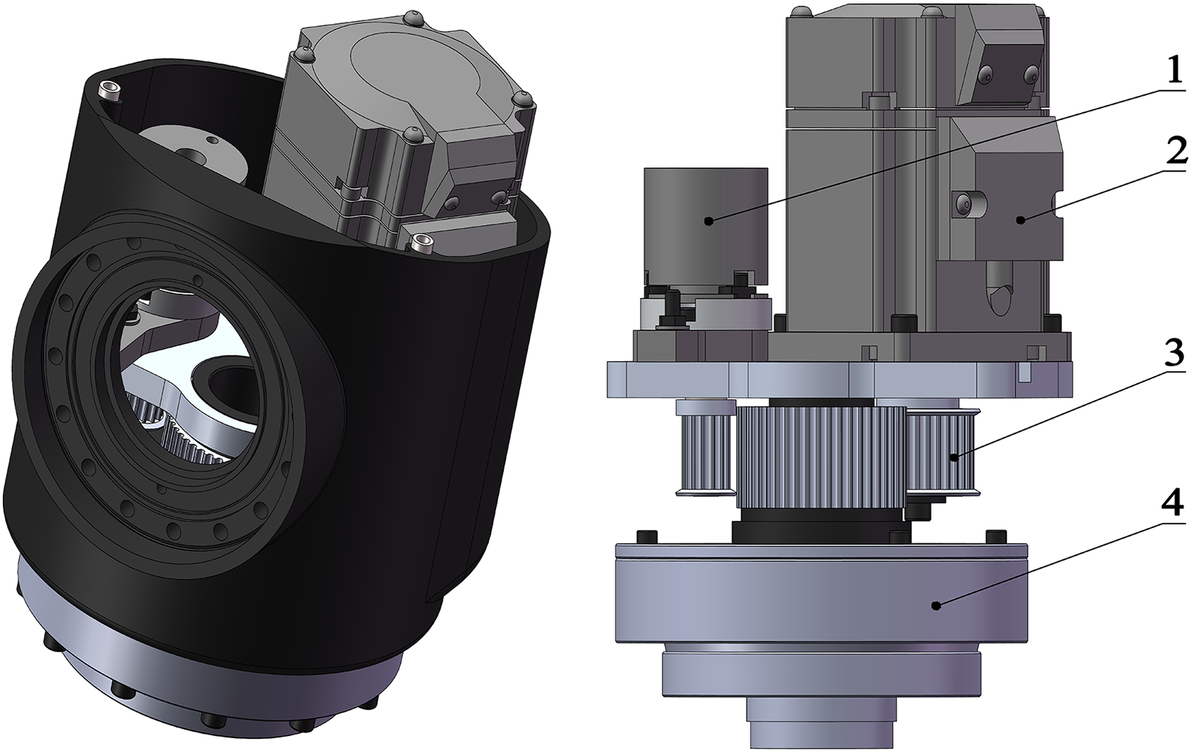
3-D joint model for the experimental robot. 1—power-off brake; 2—servo motor; 3—belt wheel; 4—harmonic reducer. 3-D: three-dimensional.

As shown in Figure 7, when the robot is running, the brake and motor charge at the same time, so the brake belt wheel is in a free state, and the reducer wheel rotation is driven by the motor wheel. When the robot stops, the brake and motor lose electricity at the same time, and without drive from the motor, the reducer wheel stops rotating because the brake wheel is fixed. The inertia tensor was measured by SolidWorks software [SolidWorks Premium 2013 SP4.0], so it’s necessary to consider inertia compensation for the rotating components. In order to acquire an accurate dynamic model of the running robot, the moment of the motor, reducer belt wheel, and other transmission segments need to be considered as equivalent to the output of the reducer for joint i. So, the inertia momentum Iz_i of joint output can be expressed by

I z_{i} = I_{reducer} + (I_{motor} + I_{belt1}) \cdot {i_{m}}^{2} + I_{belt2} \cdot {i_{b}}^{2}

where I_reducer is the inertia momentum of the reducer, I_motor is the inertia momentum of the motor, I_belt1 is the inertia momentum of the belt wheel of the motor, i_m is the reducing ratio between the belt wheel of the motor and the belt wheel of the reducer, I_belt2 is the inertia momentum of the belt wheel of the brake, and i_b is the reducing ratio between the belt wheel of the brake and belt wheel of the reducer.

Simulation using the collision detection algorithm

Our collision detection algorithm based on the momentum deviation observer was proposed above. In order to verify the model’s validity and optimize it, we simulated application of the algorithm.

Unified simulation processing was carried out in a motion/SolidWorks and a Simulink/MATLAB environment. The angles, angular velocities, and torques of the joints were obtained using simulation in the motion environment. Numerical simulation was then carried out in the Simulink environment using the motion parameters. The simulation workflow is shown in Figure 8.

Figure 8.

Simulation flow chart for collision detection.

Physical simulation was carried out in the motion environment. This has the advantage of being straightforward and comprehensive. The angle movement function was provided for each joint. The angles of the initial point and endpoint are shown in Table 2, and the whole trajectory curve for the joint is shown in Figure 9.

Table 2.

Robot angles for initial point and endpoint.

Joint	1	2	3	4	5	6
P1 (°)	0	0	0	0	0	0
P2 (°)	90	−30	100	60	−90	180

Figure 9.

Trajectory of the robot.

Collision force was added at the wrist joint as shown in Figure 10. A vertical upward force F_c equal to 10 N was added after 3 s and lasted for 1 s. The motion information and joint torques were then obtained.

Figure 10.

Schematic illustration of collision force.

The collision detection observer was built in a Simulink environment as shown in Figure 11. Then, the simulation was carried out.

Figure 11.

Collision detection observer.

Figures 12 and 13 show the collision detection observed value curves for joints 2 and 3. There is an obvious peak in both figures. The observed values tracked the actual torque curve effectively, so the algorithm was verified, showing both excellent responsiveness and accuracy.

Figure 12.

Simulation curve for observed value (joint 2).

Figure 13.

Simulation curve for observed value (joint 3).

The relationship between collision force and joint collision torque was expressed in equation (2). This can therefore be used to calculate the joint torque produced by collision force. The observed values can track joint collision torque better with adjusted parameters. In the results shown in the figures above, the parameters K₁ and K₂ were equal to 25 and 0.95, respectively.

Because there was no friction force during the simulation, the external torque was equal to the collision torque. The final overshoot of the observer model needs to be decreased as much as possible to ensure responsiveness. To this end, the parameters can be adjusted to specific working conditions, thus improving the robustness of the observer.

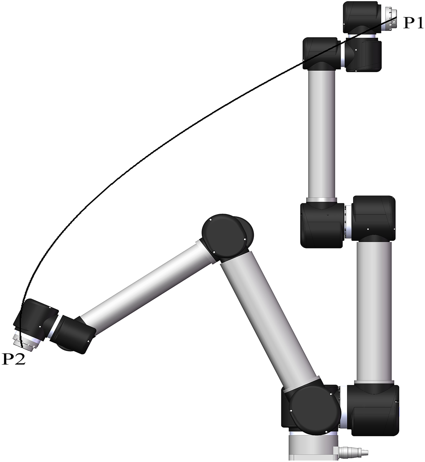
The novel detection algorithm uses joints as collision detection units. This is unaffected by the number of joints, strengthening the scope of its potential applicability. The observed values for the joints are calculated separately and a collision is considered to be happening if any joint values exceed the threshold. This makes the approach suitable for many kinds of jointed robots. In order to prove the sensitivity and scope of the algorithm, a second simulation based on the well-known 7-DOF collaborative robot KUKA (Germany) iiwa R820 was carried out. The model considered friction using the parameters obtained for the 3-D model that were modified according to the works of Jubien et al.³⁰ The coefficients of the observer were the same as in the first simulation. The trajectory was set to point–to-point mode, and the collision force was horizontal and equal to 8 N. This was applied at the sixth joint, as shown in Figure 14. The observed value curves without and after friction compensation are shown in Figures 15 and 16, respectively.

Figure 14.

KUKA iiwa R820.

Figure 15.

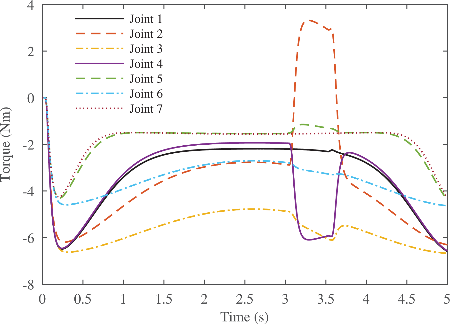
Observed value curve without friction compensation.

Figure 16.

Observed value curve after friction compensation.

It can be seen from the comparison that the collision torque was disrupted by the friction torque when there was no compensation. Additionally, the small collision force never reached the threshold value of 8 Nm. After compensation, the threshold value was set much lower (i.e. 1 Nm), and the collision was able to be detected. In fact, the threshold values for each different joint can be set to something different, thus achieving better sensitivity and overstepping any possible blocking of the collision detection.

Experimental analysis

In order to verify the practical applicability of the collision detection algorithm, an experiment was set up. The equipment used was a lab-built hollow collaborative robot as shown in Figure 17. A C# program was written in the Microsoft Visual Studio environment, which included filter processing, calculation of observed values, collision judgment, and response strategies.

Figure 17.

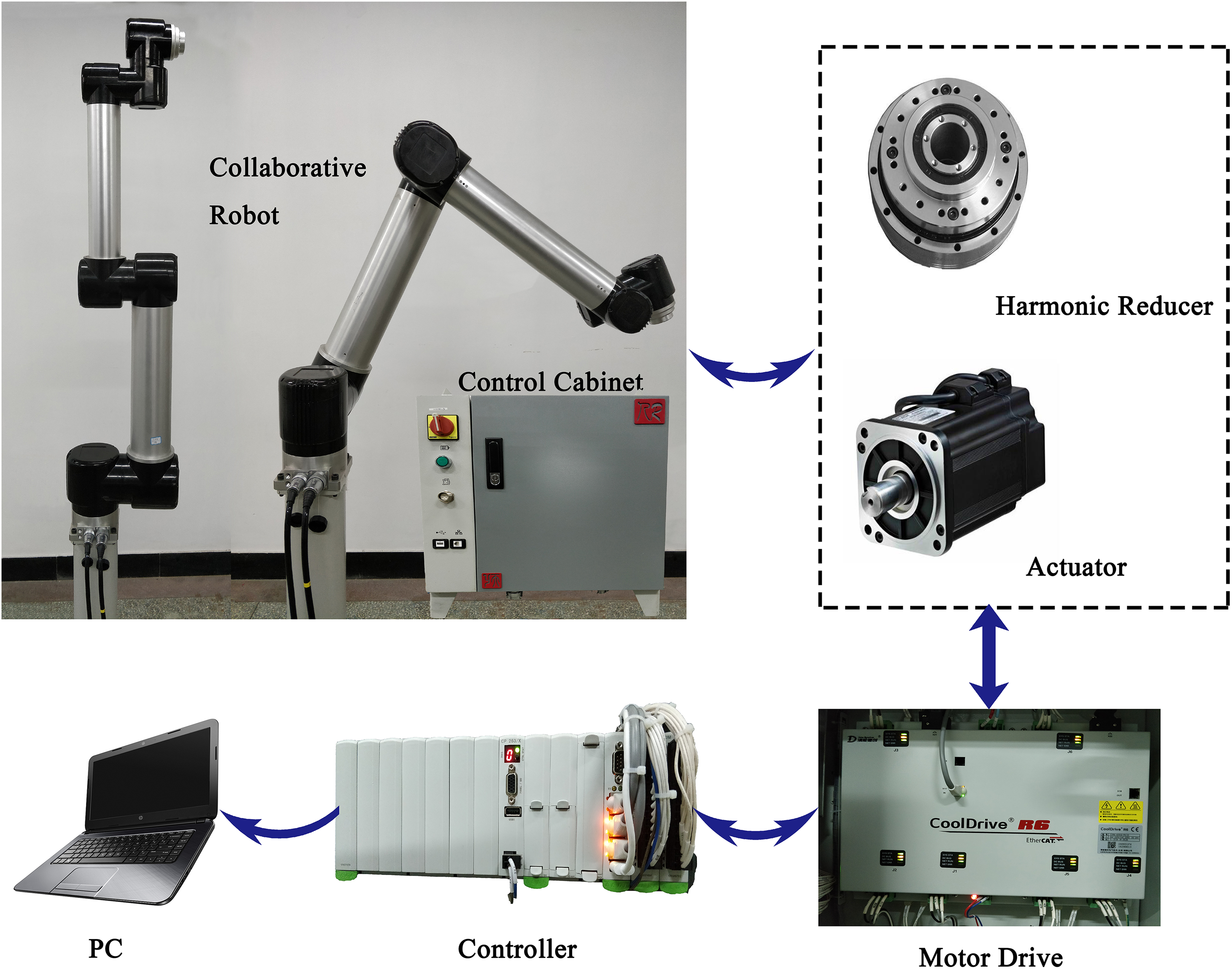
Collaborative robot experimental platform.

By producing an actual collision with a collaborative robot, it was possible to acquire final results and verify the algorithm. Robots move in different directions with different velocities and acceleration, and it is possible to get a range of observed values. The extremes of these values decide at what level the threshold value needs to be set to avoid erroneous detection without external interference.

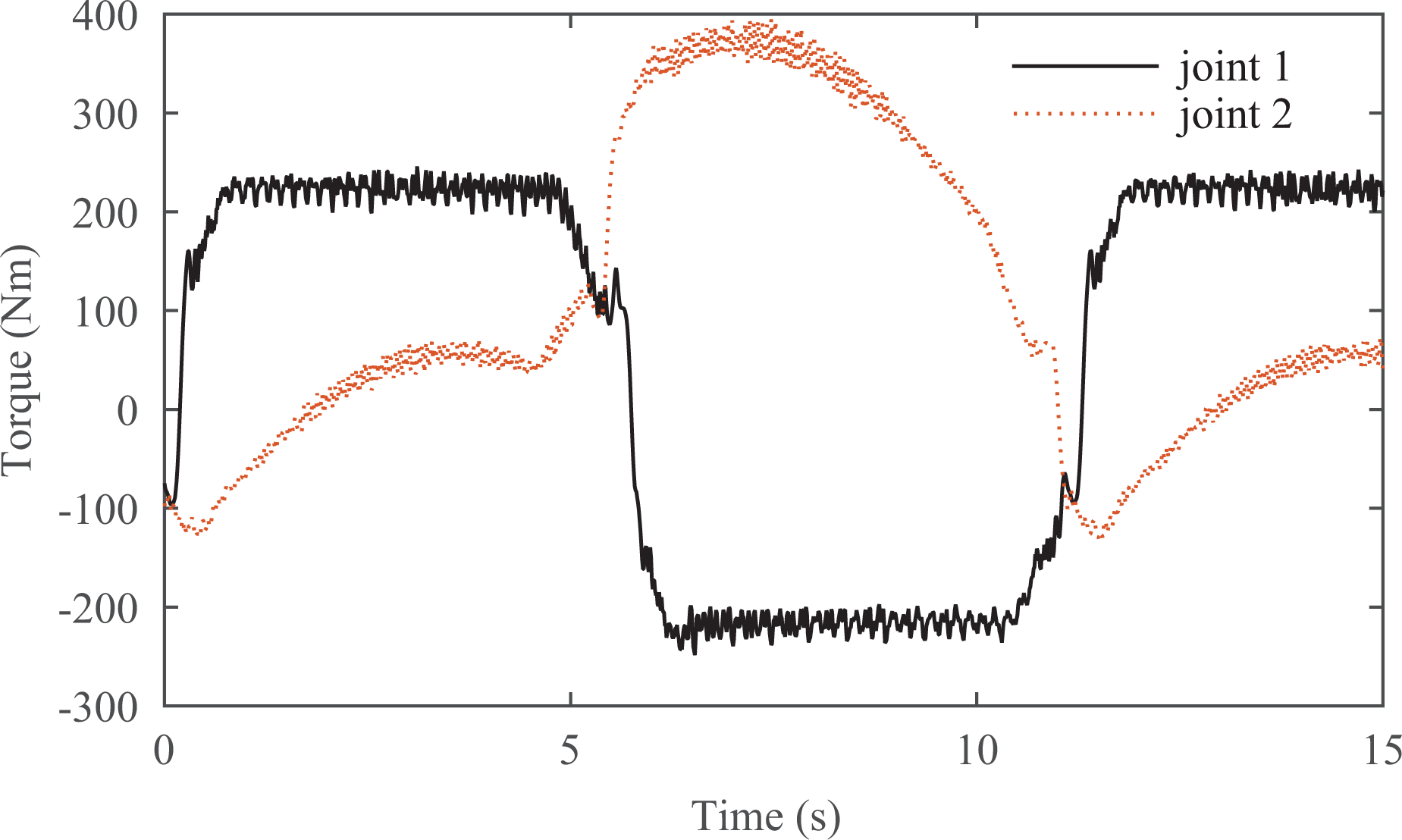
The collision experiment was conducted in the same way as the first simulation. The start and end postures for the trajectory are shown in Figure 17. The observed value curves without and after friction compensation are shown in Figures 18 and 19, respectively. When there was no compensation, the shifts in the curve are nowhere near as obvious as they are in Figure 19. According to the results, the algorithm meets the requirements effectively. If the observed value exceeded the threshold, the robot adopted a response strategy. Different response strategies produce different results, ensuring man–robot collaboration safety.

Figure 18.

Observed value curves without compensation for the experiment.

Figure 19.

Observed value curves after compensation for the experiment.

In Figure 19, joints 2 and 3 are sensitive to this type of collision force depending on its position and direction. This enables the collision position to be detected.

If the collision force was increased and the experiment rerun, the observed values increased as well. In Figure 20, the threshold value was set at 7 Nm.

Figure 20.

Comparison of observed values according to different collision forces.

As shown in Figures 21 and 22, the collision force was measured using a push-pull dynamometer (made by Yueqing Handpi Instruments Co., Ltd, China). The collision forces were measured at different tool center point (TCP) velocities using different threshold values shown in Table 3. The measurements were carried out using the algorithms with and without friction compensation, and two typical forces were applied. Joints 2 and 3 are more sensitive under vertical forces and joint 1 is more sensitive under lateral forces. The smaller the threshold values, the more easily the collision can be detected and the collision forces reduced. The threshold values can be set to be the same, because the observed values are small enough after compensation. However, the threshold value must be set differently if there is no compensation. Without compensation, the sensitivity of the observer to the forces in different directions changes. For example, the lateral negative force is equal to 38 Nm, but the positive force is up to 58 N. This is because, when the collision torque is in an opposite direction to the friction torque, the observed values decrease and the collision can’t be detected. After compensation, the sensitivity of the observer is stable, which leads to a better performance. In summary, then, the overall collision forces can be affected by the threshold values, the force types, and the velocities of the TCP. The forces were measured 10 times for each velocity and calculated in average. The experiment verified that the actual measured average collision forces were lower than the human tolerance limit of 65–165 N, so safety can be ensured.

Figure 21.

Collision force measurement.

Figure 22.

Collision force curve measured by the dynamometer.

Table 3.

Average collision forces under different conditions.

Collision force	Threshold value(Nm)\TCP velocities (mm s⁻¹)	After friction compensation			No friction compensation¹⁶
Collision force	Threshold value(Nm)\TCP velocities (mm s⁻¹)	7	20	35	Set separately
Vertical force (N)	100(+)	14.92	16.87	23.17	19.28
	250(+)	21.25	22.13	27.43	25.37
	350(+)	31.74	35.47	40.58	33.53
	450(+)	40.43	40.58	52.60	46.73
	550(+)	49.36	56.87	59.77	51.64
	350(−)	34.13	39.62	47.67	49.75
Lateral force (N)	350(+)	36.77	37.68	49.18	58.37
Lateral force (N)	350(−)	34.91	37.73	48.75	38.16

TCP: tool center point.

Conclusion

In order to ensure the safety of human interactions with collaborative robots, a collision detection algorithm was proposed that takes friction into account. The algorithm can detect collisions without changing a robot’s physical structure and adding external sensors. The algorithm displays good accuracy and real-time performance. The associated model is able to adjust parameters and achieve both excellent responsiveness and decreased overshoot. A friction compensation model was adopted that considers the actual running condition of the robot in order to ensure that observed values are only affected by collision torque. The inertial forces produced by rotating components were compensated for using software analysis, thereby achieving the goal of improved accuracy for both the dynamic model and the collision detection algorithm. Filter processing was used to reduce high frequency noise, thus eliminating interference from other factors and enhancing reliability. Using software simulation and actual experiments, the collision detection algorithm was shown to track collision torque effectively. Observed values fluctuate around 0 without collision. A suitable threshold values were set to make the robot run normally under non-collision conditions. The algorithm uses joints as detection units, so that a variety of response strategies can be established. The algorithm has a simple structure and wide adaptability, so its application value is significant.

Footnotes

Acknowledgements

The authors gratefully acknowledge Zhitao Zhang, Hongye Liu, and Wenbin Duan of Tianjin Yangtian Technology Co., Ltd for their helpful discussion.

Declaration of conflicting interests

The author(s) declared no potential conflicts of interest with respect to the research, authorship, and/or publication of this article.

Funding

The author(s) disclosed receipt of the following financial support for the research, authorship, and/or publication of this article: This study was supported in part by the major projects of Tianjin intelligent manufacturing science and technology (grant no.16ZXZNGX00140) and the National Natural Science Foundation of China (grant no. 91648202).

ORCID iD

Qiulong Zhang

References

Bicchi

Bavaro

Boccadamo

. Physical human-robot interaction: dependability, safety, and performance. In: AMC ‘08: 2008 10th IEEE international workshop on advanced motion control (1–2), Trento, Italy, 26–28 March 2008, pp. 9–14. IEEE.

Pedrocchi

Vicentini

Matteo

. Safe human-robot cooperation in an industrial environment. Int J Adv Robot Syst 2013; 10. DOI: 10.5772/53939.

Haddadin

Albu-Schaffer

Frommberger

. The “DLR Crash Report”: towards a standard crash-testing protocol for robot safety – part II: discussions. In: ICRA: 2009 International Conference on Robotics and Automation, Vol. 1–7, Kobe, Japan, 12–17 May 2009, pp. 280–287. IEEE.

De Luca

Mattone

. Sensorless robot collision detection and hybrid force/motion control. In: 2005 2009 International Conference on Robotics and Automation, Vol. 1–4, Barcelona, Spain, 18–22 April 2005, pp. 999–1004. IEEE.

Povse

Koritnik

Kamnik

. Industrial robot and human operator collision. In: IEEE international conference on systems, man and cybernetics (SMC 2010), Istanbul, Turkey, 10–13 October 2010.

Ebert

Henrich

. Safe human-robot-cooperation: image-based collision detection for industrial robots. In: 2002 International conference on intelligent robots and systems, proceedings, Vol. 1–3, Lausanne, Switzerland, 30 September–4 October 2002, pp. 1826–1831. IEEE.

Zhu

Liu

. A flexible capacitive tactile sensor for robot skin. In: IEEE ICARM 2016 – 2016 international conference on advanced robotics and mechatronics (ICARM), Macau, China, 18–20 August 2016, pp. 207–212. IEEE.

Cao

. A laser-based multi-robot collision avoidance approach in unknown environments. Int J Adv Robot Syst 2018; 15. DOI: 10.1177/1729881418759107.

Chung

Velinsky

. Human-robot collision detection and identification based on wrist and base force/torque sensors. In: Proceedings – IEEE international conference on robotics and automation, Barcelona, Spain, 18–22 April 2005, pp. 3796–3801. IEEE.

10.

Chung

. Collision detection enabled weighted path planning: a wrist and base force/torque sensors approach. In: 2005 12th international conference on advanced robotics, Seattle, WA, USA, 18–20 July 2005, pp. 165–170. IEEE.

11.

Park

Kim

Song

. Safe robot arm with safe joint mechanism using nonlinear spring system for collision safety. In: ICRA: 2009 IEEE international conference on robotics and automation, Vol. 1–7, Kobe, Japan, 12–17 May 2009, pp. 571–576. IEEE.

12.

Yamada

Hirasawa

Huang

. Human-robot contact in the safeguarding space. IEEE/ASME Trans Mech 1997; 2(4): 230–236. DOI: 10.1109/3516.653047.

13.

Haddadin

Albu-Schäffer

Hirzinger

. Safety evaluation of physical human-robot interaction via crash-testing. In: Robotics: Science and Systems, Atlanta, GA, USA, 27–30 June 2007, pp. 217–224. MIT Press.

14.

De Luca

Albu-Schäffer

Haddadin

. Collision detection and safe reaction with the DLR-III lightweight manipulator arm. In: IEEE International Conference on Intelligent Robots and Systems, Beijing, China, 9–15 October 2006, pp. 1623–1630. IEEE.

15.

De Luca

Mattone

. Actuator failure detection and isolation using generalized momenta. In: Proceedings – IEEE international conference on robotics and automation, Taipei, Taiwan, 14–19 September 2003, pp. 634–639. IEEE.

16.

. A momentum-based collision detection algorithm for industrial robots. In: 2015 IEEE international conference on robotics and biomimetics, IEEE-ROBIO, Zhuhai, China, 9–6 December 2015, pp. 1253–1259. IEEE.

17.

D’Ippolito

Alonge

Cucco

. Contact estimation in robot interaction. Int J Adv Robot Syst 2014; 11. DOI: 10.5772/58688.

18.

Cho

Kim

. Collision detection algorithm to distinguish between intended contact and unexpected collision. Adv Robot 2012; 26(16): 1825–1840. DOI: 10.1080/01691864.2012.685259.

19.

Lee

Song

. Sensorless collision detection based on friction model for a robot manipulator. Int J Prec Eng Man 2016; 17: 11–17. DOI: 10.1007/s12541-016-0002-3.

20.

Lee

Kim

Song

. Sensorless collision detection for safe human-robot collaboration. In: 2015 IEEE/RSJ international conference on intelligent robots and systems (IROS), Hamburg, Germany, 28 September–2 October 2015, pp. 2392–2397. IEEE.

21.

Chen

Luo

. A universal algorithm for sensorless collision detection of robot actuator faults. Adv Mech Eng 2018; 10: 1–10. DOI: 10.1177/1687814017740710.

22.

Craig

. Introduction to robotics: mechanics and control, 3rd ed. Boston, USA: Addison-Wesley Pub. Co., 2005, pp. 263–264.

23.

Murray

Sastry

A mathematical introduction to robotic manipulation. Boca Raton, USA: CRC Press Inc, 1994, p. 292.

24.

Zheng

. Parameter identification of LuGre friction model for robot joints. Adv Mater Res 2012; 479–481: 1084–1090. DOI: 10.4028/www.scientific.net/AMR.479-481.1084.

25.

Han

Lee

. Friction and uncertainty compensation of robot manipulator using optimal recurrent cerebellar model articulation controller and elasto-plastic friction observer. IET Control Theory A 2011; 5(18): 2120–2141. DOI: 10.1049/iet-cta.2010.0389.

26.

Grami

Gharbia

. GMS friction compensation in robot manipulator. In: IECON 2013 – 39th annual conference of the IEEE industrial electronics society, Vienna, Austria, 10–13 November 2013, pp. 3555–3560. IEEE.

27.

Martinez-Rosas

Alvarez-Icaza

Noriega-Pineda

. Model-based dynamic friction compensation in robot actuators. Int J Robot Autom 2015; 30: 1–12. DOI: 10.2316/Journal.206.2015.1.206–3607.

28.

Welch

Bishop

. An introduction to the Kalman filter. Chapel Hill: University of North Carolina, 2013, pp. 127–132.

29.

Gandhi

Ghorbel

Dabney

. Modeling, identification, and compensation of friction in harmonic drives. In: Proceedings of the IEEE conference on decision and control, Las Vegas, NV, USA, 10–13 December 2002, pp. 160–166. IEEE.

30.

Jubien

Gautier

Janot

. Dynamic identification of the KUKA lightweight robot: comparison between actual and confidential KUKA’s parameters. In: 2014 IEEE/ASME international conference on advanced intelligent mechatronics, Besacon, France, 8–11 July 2014, pp. 483–488. IEEE.

Collision detection algorithm for collaborative robots considering joint friction

Abstract

Keywords

Introduction

External torque observer

Design of the external torque observer

Algorithmic optimization

Identifying friction in the joint

Building the friction model

Friction identification experiment

Filtering preprocessing

Joint friction identification

Collision detection algorithm

Algorithm construction and inertia compensation

Simulation using the collision detection algorithm

Experimental analysis

Conclusion

Footnotes

Acknowledgements

Declaration of conflicting interests

Funding

ORCID iD

References