Sage Journals: Discover world-class research

Abstract

Chinese river crabs are important aquatic products in China, and the accurate operation of aquatic plants cleaning workboat is an urgent need for solving various problems in the aquaculture process. In order to achieve the accurate navigation positioning, this article introduces the visual-aided navigation system and combines the advantages of particle filter in nonlinear and non-Gaussian systems. Meanwhile, the generalized regression neural network is used to adjust the particle weights so that the samples are closer to the posterior density, thus avoiding the phenomenon of particle degradation and keeping the diversity of particles. In order to improve the network performance, the fruit fly optimization algorithm is introduced to adjust the smoothing factor of transfer function for the generalized regression neural network model layer. On this basis, the location filtering navigation method based on fruit fly optimization algorithm-generalized regression neural network-particle filter is proposed. According to the simulation results, the mean_R of root-mean-square error of the proposed fruit fly optimization algorithm-generalized regression neural network- particle filter method decreases by 12.39% and 6.87%, respectively, compared with those of particle filter and generalized regression neural network methods, and the mean_T of running time decreases by 16.04% and 9.14%, respectively. From the repeated experiments on the aquatic plants cleaning workboat in crab ponds, the latitude error of the proposed method decreases by 23.45% and 12.68%, respectively, and that the longitude error decreases by 29.11% and 17.65%, respectively, compared with those of particle filter and generalized regression neural network methods. It is proved that our proposed method can effectively improve the navigation positioning accuracy of aquatic plants cleaning workboat.

Keywords

Crab farming aquatic plants cleaning workboat visual navigation particle filter generalized regression neural network fruit fly optimization algorithm

Introduction

As an important aquaculture species in China, Chinese river crabs are rich in nutrition and have high economic value.^1,2 In the process of river crab farming, farmers generally take the aquaculture mode of planting aquatic plants. Aquatic plants not only provide favorite food and habitats for crabs but also improve the survival environment of crabs through increasing the dissolved oxygen level, decreasing harmful substances, adsorbing heavy metals, and purifying the water.^3,4 In river crab farming, the general required height from the top of aquatic plants to water surface is about 20 cm. In view of this, the cleaning and maintenance of aquatic plants always play a key role in successful crab farming.⁵

At present, the cleaning of aquatic plants in river crab farming is mainly accomplished through manual operation, which means heavy labor intensity and high cost.⁶ In order to reduce the labor intensity, it is of great significance to design an intelligent automatic workboat for cleaning aquatic plants in crab farming. Currently, the aquatic plants cleaning workboat mainly relies on the global positioning system (GPS) navigation mode.⁷ However, under this kind of navigation mode, the workboat can only navigate along the preset artificial route, whereas aquatic plants are not always in the preset route. As a result, the errors between the workboat sailing trajectory and actual aquatic positioning are usually large, and the cleaning effect on aquatic plants is not desirable. In this study, a more advanced visual navigation is introduced to obtain the visual information through the camera and complete the auxiliary navigation work.⁸ Visual navigation is a hot issue in current navigation research, especially in agricultural machinery. In the navigation route extraction algorithm of visual navigation system, a navigation route detection method based on improved genetic algorithm was proposed. Genetic optimization selected the individuals with the highest fitness as the straight line coding of crops and then got the navigation line.⁹ In order to effectively and quickly identify the navigation and location of parallel lines in farmland, a parallel line recognition based on machine vision was proposed, and an improved parallel recognition algorithm based on Hough transform was used to identify and locate ridge lines.¹⁰ Meanwhile, in order to ensure the system reliability in the complex background environment of aquaculture ponds, this study combines the advantages of visual navigation and GPS navigation and establishes an integrated navigation method to improve the positioning accuracy and workboat efficiency.^11,12

In navigation and positioning filtering, the particle filter (PF) method is often used to improve positioning accuracy and reduce positioning error.^13,14 PF is a kind of filtering technique based on Monte Carlo’s thought,¹⁵ and its state function and observation function are both based on nonlinear and non-Gaussian hypothesis. Hence, this method is widely used in the field of nonlinear and non-Gaussian navigation and target tracking.^16,17 Gordon et al. proposed a resampling algorithm. However, this method can easily lead to particle depletion and thus affect the accuracy of particle filtering.¹⁸ Torma and Szepesvári proposed an adaptive adjustment PF algorithm based on likelihood distribution.¹⁹ The algorithm selected the importance density function as the priori density and neglected the influence of the latest measurement information in the system. Although the filtering stability was improved to some extent, new particles would be generated when the non-normalized likelihood function values were more than the preset threshold. So the navigation accuracy was relatively low. Zhao et al. proposed a fast quasi-Monte Carlo (QMC)-based PF algorithm. However, this method relied on the spatial location of the parent particle, and the selection of the subspace size still needed to be optimized.²⁰ Guo and Wang proposed a sequential QMC algorithm to achieve higher estimation accuracy by randomizing the QMC samples in the sample space, but this method had too high computational complexity for convenient applications.²¹ In the study by Talantzis,²² a novel speaker tracking framework of PF based on information theory was discussed. In the study by Zhong et al.,²³ an extended Kalman particle filtering (EKPF) approach for tracking nonconcurrent multiple talkers was proposed. Furthermore, a decentralized particle filter (DPF) method was presented based on the consensus filter over sensor networks to implement tracking task, in which each node performs a local PF and only interacts with its neighbor nodes to calculate a global state estimation.²⁴ Actually, DPF methods are more robust than the centralized PF ones.

Particle depletion and diversity issues are the main problems that affect the accuracy and localization of particle filtering. In order to solve these problems, intelligent algorithms are often introduced to optimize the PF. In navigation and positioning, the optimized particle filtering method is a hot research topic. Firefly algorithm is a popular intelligent optimization algorithm in recent years, which is proposed by Professor Yang of Cambridge University in 2009.²⁵ On this basis, Tian et al. proposed a PF based on firefly algorithm optimization, which dynamically optimized the particle set through brightness and attractiveness so as to solve the problem of particle depletion caused by resampling.²⁶ Chen et al. proposed a bat algorithm-optimized PF algorithm.²⁷ The simulation results show that this algorithm is superior to other population intelligent optimization algorithms. However, based on the population optimization algorithm, the optimal particles number of PF is set to a priori fixed value. But in actual use, in order to ensure the performance of the algorithm, a larger particle sampling size is usually used. As a result, the efficiency of the algorithm drops drastically. Due to the weighted summation step of the PF, much redundant particles would lead to the decrease of the calculation accuracy. At present, many advanced intelligent algorithms were used to optimize particle filtering and apply it to the research of navigation and positioning, especially in the applications of robots, target tracking, and so on. However, many optimization algorithms are still difficult to meet the system’s requirements, so the problem of navigation of the optimized PF deserves further study.

With the development of neural network technology, it is also a hot topic in the research of the optimization of PF. Tyan and Kim proposed a compact convolutional neural network (CNN)-based tracker in conjunction with a PF architecture. This method had higher positioning accuracy for the target tracker of motion, but because of the introduction of convolution operations, the amount of calculation was relatively large and the efficiency of the algorithm need to be improved.²⁸ Chen et al. proposed a new method, which used generalized regression neural network (GRNN) to calculate the weights of the offsprings. It can improve the precision and the speed of the filter. The experimental results showed that the algorithm can be used to track the radar target with higher computational accuracy than the standard QMC PF. However, the method did not optimize the transfer function of the model layer in the network, and it affects the performance of the network to some extent, so the stability of GRNN needs to be improved.²⁹ As a new intelligent algorithm, the fruit fly optimization algorithm (FOA) was appeared in recent years, which was put forward by Pan in 2012.³⁰ It has many advantages, such as the amount of calculation is smaller, operation time is shorter, and optimization precision is higher.³¹ In this study, we introduced the FOA to optimize the GRNN network, which was used to improve the stability of GRNN.

For the above-mentioned tracking methods based on the PF or DPF, the variance of particle weights generally increases with time extension. As a result, traditional PF methods in the positioning filter often encounter the phenomenon of particle depletion, which greatly affect the accuracy of state estimation.³² In this study, the importance density function is optimized by GRNN firstly.³³ Then, after the prediction step, in order to improve the filtering accuracy, the sample is adjusted by GRNN so that it is closer to the posterior density. For the model layer of GRNN, the smoothing factor of the transfer function has a great influence on the operation of network performance, so this study introduces the FOA to adjust the smoothing factor of GRNN in the space optimization.³⁰ In this study, an FOA method is proposed to adjust the smoothing factor of GRNN, and then PF is optimized to obtain the aquatic cleaning workboat navigation filtering method (FOA-GRNN-PF). Furthermore, the proposed method is verified through simulation and navigation experiments.

The rest of this article is organized as follows. “Materials and methods” section establishes the system model and the coordinate system and describes the principles of the FOA-GRNN-PF method. In “Experimental results and discussion” section, the performance results and related analysis are given from three aspects of image processing experiment, simulation experiment, and navigation experiment. Especially in the simulation, navigation experiment, and result analysis, the proposed method is compared with PF and GRNN-PF methods. Finally, some conclusions and suggestions for further work are summarized in “Conclusions and future work” section.

Materials and methods

System model

In order to obtain accurate navigation and positioning effect, an optimized PF is used to locate and filter the integrated navigation.³⁴ Hence, the basic model of the system should be established firstly. The most important thing is to obtain the location information of the aquatic plants-cleaning workboat. Since the workboat sails in the crab pond, it can be approximated as a pure azimuth tracking model. Thus, the state equation and the measurement equation can be established by the target position and velocity as follows.

State equation

For studying the aquatic plants-cleaning workboat, it is necessary to establish the visual coordinate system and the world coordinate system when the workboat is sailing. The coordinate system is established as shown in Figure 1.

Figure 1.

The coordinate system.

In Figure 1, we select the current location and the target location of the workboat as the objects. For generating the navigation point, it is actually the position information of the workboat and target location. We assume that the state vector of the navigation system is X_k, and then the system state equation can be defined as follows

X (k) = ϕ X (k - 1) + ψ Η (k - 1)

In the process of establishing the navigation system model of this study, the position information is obtained through the state equation. And the state equation is composed of $x_{c} (k T), y_{c} (k T), u_{x_{k}}, v_{y_{k}}, x_{p} (k T)$ , and y_p(k_T). $x_{c} (k T), y_{c} (k T)$ are the coordinate values of the target in the coordinate system X and Y, respectively, which can be obtained in real time through GPS; u_xk and v_yk represent the speed of the workboat corresponding to the coordinate system X and Y, respectively, which are also acquired by the GPS model. x_p(k_T) and y_p(k_T) represent the position coordinates of the target point in the coordinate system X and Y, respectively. The vision system can calculate the coordinate position of the target point through the obtained image information and the camera parameters.

In formula (1), T is the sampling period and k = 1, 2, ⋯ n. ϕ represents a state transition matrix from the time k − 1 to k. ψ represents the system state noise matrix. ϕ and ψ are, respectively, as follows

ϕ = [\begin{matrix} 1 & 0 & T & 0 & 0 & 0 \\ 0 & 1 & 0 & T & 0 & 0 \\ 0 & 0 & 1 & 0 & 0 & 0 \\ 0 & 0 & 0 & 1 & 0 & 0 \\ 0 & 0 & 0 & 0 & 1 & 0 \\ 0 & 0 & 0 & 0 & 0 & 1 \end{matrix}]

ψ = [\begin{matrix} 1 & 0 \\ 0 & 1 \\ 1 & 0 \\ 0 & 1 \\ 1 & 0 \\ 0 & 1 \end{matrix}]

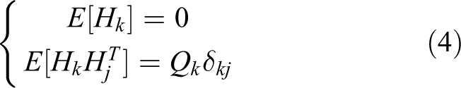
Moreover, $H (k - 1) = {[\begin{matrix} {H_{x}}_{_{k - 1}} & {H_{y}}_{_{k - 1}} \end{matrix}]}^{T}$ represents the model error and system noise caused by disturbance. ${H_{x}}_{_{k - 1}}$ and ${H_{y}}_{_{k - 1}}$ , respectively, denote the system noise in the X and Y directions at time k−1. Among them, the system noise is zero-mean Gaussian white noise, which satisfies the following formula

{\begin{matrix} E [H_{k}] = 0 \\ E [H_{k} H_{j}^{T}] = Q_{k} δ_{k j} \end{matrix}

where Q_k denotes the symmetric nonnegative variance matrix of system noise, δ_kj is the function of Kronecker-δ, E[H_k] is the mean of system noise, and $E [H_{k} H_{j}^{T}]$ is the system noise variance estimation matrix.

Measurement equation

In Figure 1, the angle between $\vec{P G}$ and $\vec{P Q}$ is defined as the azimuth, which is denoted as θ. It can be calculated as follows

θ (k T) = arctan (\frac{x_{p} - x_{c}}{y_{p} - y_{c}})

Then, the measurement equation of the operating vessel navigation system can be expressed as

θ (k T) = arctan (\frac{x_{p} - x_{c}}{y_{p} - y_{c}}) + v (t)

where ν(k) is the system measurement noise. Among them, the system measurement noise is zero-mean Gaussian white noise, which satisfies the following formula

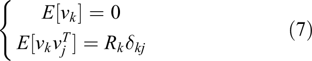
{\begin{matrix} E [v_{k}] = 0 \\ E [v_{k} v_{j}^{T}] = R_{k} δ_{k j} \end{matrix}

where R_k denotes the variance matrix of measurement noise; and δ_kj is the function of Kronecker-δ.

Principles of FOA-GNRR-PF

PF is a widely used filtering method in related studies of navigation and positioning. Its basic idea is resampling algorithm that PF samples with large weights will be repeated, whereas small-weight samples will be directly discarded. This feature of PF not only easily leads to particle depletion but also results in the loss of particle diversity.³⁵ To avoid the phenomenon of particle depletion and maintain particle diversity, GRNN is introduced to adjust particle weights so that the samples can be made closer to the posterior density. For GRNN parameters, we only need to adjust the smoothing factor σ in the model kernel function, since the suitable σ value has a great influence on the GRNN performance. In this study, we introduce FOA in the spatial search to find the best σ value using the keen sense of smell and visual function of fruit fly.

Basic principles of PF

PF is an approximate Bayesian filtering algorithm based on Monte Carlo’s idea.³⁶ This method uses a number of discrete and random particles to approximate the probability density function of random variables in the system and replaces the integral operation by averaging the samples to obtain the minimum variance estimate of the state. The Monte Carlo method collects the weight of particle sets (sample sets) from the posteriori probability sampling, and then uses the particle sets to represent the posterior distribution.^16,24

In two-dimensional target positioning system, according to the state equation (1) and the measurement equation (5) of the workboat system, PF algorithm is implemented, which is as follows:

Step 1. Sampling

In this study, the prior probability density function is chosen as the importance function, and its expression formula is

X_{k}^{i} \sim P (X_{k} | X_{k - 1}^{(m)})

After sampling, we get the particle setting as ${{X_{k}}^{(m)}}_{m = 1}^{N}$ at the time k, m = 1, 2, ⋯, N. The workboat state formulas are as follows

x_{c, k}^{(m)} = x_{c, k - 1}^{(m)} + u_{x_{k - 1}}^{(m)} + H_{x_{k - 1}}^{(m)}

y_{c, k}^{(m)} = y_{c, k - 1}^{(m)} + u_{y_{k - 1}}^{(m)} + H_{y_{k - 1}}^{(m)}

u_{x_{k}}^{(m)} = u_{x_{k - 1}}^{(m)} + H_{x_{k - 1}}^{(m)}

v_{x_{k}}^{(m)} = v_{x_{k - 1}}^{(m)} + H_{y_{k - 1}}^{(m)}

x_{p, k}^{(m)} = x_{p, k - 1}^{(m)} + H_{x_{k - 1}}^{(m)}

y_{p, k}^{(m)} = y_{p, k - 1}^{(m)} + H_{y_{k - 1}}^{(m)}

Step 2. Normalized weight calculation

In this system, the measurement noise is set to zero mean Gaussian white noise. The weight is calculated as

\begin{array}{l} w_{k}^{(m)} = w_{k - 1}^{(m)} p (θ_{k} {| x}_{k}^{(m)}) \\ = w_{k - 1}^{(m)} \frac{1}{\sqrt{2 π δ_{v}^{2}}} exp {- \frac{1}{2 δ_{v}^{2}} [θ_{k} - arctan (\frac{x_{p, k}^{(m)} - x_{c, k}^{(m)}}{y_{p, k}^{(m)} - y_{c, k}^{(m)}})]} \end{array}

When the weight of each particle is calculated, the weights are normalized as

{w_{k}^{(m)}}^{*} = \frac{w_{k}^{(m)}}{\sum_{m = 1}^{N} w_{k}^{(m)}}

Step 3. Re-sampling

The resampling algorithm is used to get a new set of particles ${{\tilde{X}}_{k}^{(m)}, {\tilde{w}}_{k}^{(m)}}_{m = 1}^{N}$ .

Step 4. Estimate of output state

The position coordinate of the workboat, the speed values in the X and Y directions, and the values of the target point position coordinate are determined as follows:

{\hat{x}}_{c, k}^{(m)} = \sum_{m = 1}^{N} {w_{k}^{(m)}}^{*} x_{c, k}^{(m)}

{\hat{y}}_{c, k}^{(m)} = \sum_{m = 1}^{N} {w_{k}^{(m)}}^{*} y_{c, k}^{(m)}

{\hat{u}}_{c, k}^{(m)} = \sum_{m = 1}^{N} {w_{k}^{(m)}}^{*} u_{c, k}^{(m)}

{\hat{v}}_{c, k}^{(m)} = \sum_{m = 1}^{N} {w_{k}^{(m)}}^{*} v_{c, k}^{(m)}

{\hat{x}}_{p, k}^{(m)} = \sum_{m = 1}^{N} {w_{k}^{(m)}}^{*} x_{p, k}^{(m)}

{\hat{y}}_{p, k}^{(m)} = \sum_{m = 1}^{N} {w_{k}^{(m)}}^{*} y_{p, k}^{(m)}

Through the PF algorithm, the structure of the workboat navigation and positioning filtering system can be described as follows: Firstly, the PF system initializes the samples. The system determines the prior probability of the target state and assigns the corresponding initial value to each particle. At the next moment, the system carries out the transfer of running state and spreads its own state according to the state transition equation. The system is monitored to get the observed value, and the weights of all particles are calculated. Finally, the weights of all particles are obtained, and the output of the posterior probability is accomplished. After the sample is resampled, the system state is transferred to form a navigation positioning and filtering system.

By the above analysis, we can find that the adjustment of the weight is the key technology in the process of PF, which is the only input value in the whole algorithm. It is the azimuth of the target in the system. Each time a value of θ is entered, in order to obtain a state estimate, it will go through four steps: sampling, normalization weight calculation, resampling, and output of the state estimate. According to the whole algorithm steps, we know that for each measured value we need to deal with a large number of particles, and there are more steps to be performed. If the number of particles is large, the amount of algorithm calculation is also large, and the computation speed will be slower. To speed up the algorithm operation, it will sacrifice the diversity of particles, so it will be easy to cause particle depletion phenomenon.

FOA-GRNN network structure

By measuring the workboat azimuth to adjust the corresponding weights, it will greatly influence the speed and efficiency of the algorithm. But the GRNN has certain advantage in optimization PF. In this study, GRNN is introduced to adjust particle weights. After adjustment, the samples can be closer to the posterior density, thus avoiding particle dilution and maintaining particle diversity. GRNN is similar in structure to radial basis function neural network. It can be divided into four layers including input layer, pattern layer, summation layer, and output layer. The unit of the input layer is a simple linear unit. The model layer is also called the implicit regression layer, in which each unit corresponds to a training sample. The summation layer is composed of two units, of which one unit calculates the weighted sum of the output of each neuron in the model layer and the other calculates the sum of the output of each neuron in the pattern layer. The output layer divides the summation layer molecule unit by the denominator unit to obtain the output values.³⁷

The work process of GRNN does not need to adjust the weight between the layers. It only needs to adjust the parameters of the model layer transfer function, that is, the smooth factor σ. This parameter has a great impact on the network performance.^38,39 In this article, we try to introduce the FOA algorithm in the space search optimization, and the smoothing factor σ is used as the taste concentration judgment value S_i. Here, the mean square error (MSE) of the network target value and the actual value is the taste concentration judgment function, and it is also defined as the fitness function. Using the sensory smell and visual function of fruit fly, the smoothing factor σ is dynamically adjusted to optimize the GRNN model. The GRNN model is shown in Figure 2.

Figure 2.

Structural model of FOA to adjust the GRNN’s smoothing factor. FOA: fruit fly optimization algorithm; GRNN: generalized regression neural network.

In the training procedure of GRNN, the number of hidden layer neurons and the connection weights between layers are uniquely determined by the training samples. The value of the smoothing factor σ directly affects the performance of the neural network, so the training procedure of the network is to search the optimal smooth factor σ value. We assume that the position of the fruit fly in the three-dimensional space is ${Fly}_{(i)} (x_{i}, y_{i}, z_{i})$ , and then the distance between an individual fly and the origin is

D_{i} = \sqrt{x_{i}^{2} + y_{i}^{2} + z_{i}^{2}}

In the training process of the network, the corresponding S_i of fruit fly individuals are brought into the GRNN model as the smoothing factor σ, that is, the network model is obtained through the training sample of the network. Then, the difference between the target value and the actual measurement value of the training sample is calculated, which is used as the taste concentration of fruit fly individuals. The calculation formula is

S (i) = MSE (i) = \frac{1}{n} \sum (y_{output} - y)

where y_output is the output value, and y is the target value.

The number of neurons in GRNN is equal to the number of samples n, and the transfer function of each neuron is

P_{i} = exp [- \frac{{(X - X_{i})}^{T} (X - X_{i})}{2 σ^{2}}]

The taste concentration determination function is calculated to determine whether the current best taste concentration is better than the previous iteration of the best taste concentration. And the coordinates of best smoothing factor σ are reserved. Finally, according to the optimal σ value, determine whether the maximum number of iterations is satisfied. If yes, it substitutes into GRNN to optimize PF location filter, and the test samples and measured values can output.

FOA can optimize GRNN to obtain the best σ value, and then the best σ substitutes GRNN to optimize PF location filter. The flow chart is shown in Figure 3.

Figure 3.

FOA-GRNN flow chart. FOA: fruit fly optimization algorithm; GRNN: generalized regression neural network.

Procedure of the FOA-GRNN-PF algorithm

The proposed method can avoid the phenomenon of particle dilution and keep the diversity of particles. It can realize information sharing between particles, thus enhancing the global optimization ability of the algorithm and improving the efficiency of the filtering algorithm. In the workboat positioning system, the steps of this algorithm are as follows:

Step 1. Particle sample initialization

At the initial moment, N particles are sampled as the initial particles of the algorithm. The importance density function is represented by the formula (8).

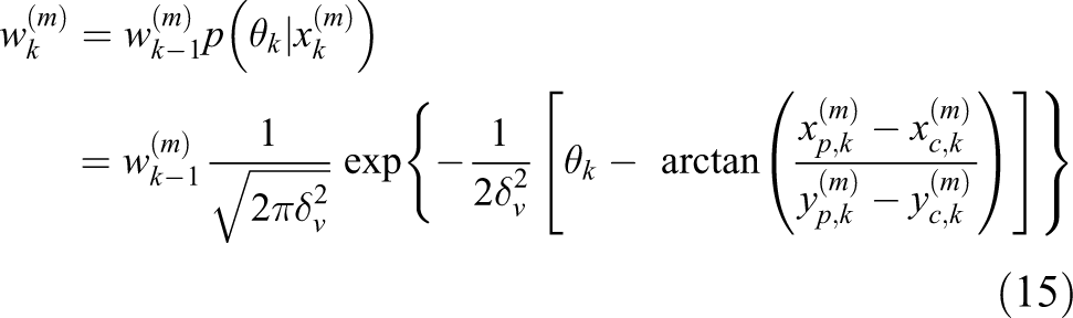
Step 2. Calculate the importance of the weight of each particle

It is calculated using formula (15).

Step 3. Optimize GRNN parameters according to FOA

Randomly generate the initial position, individual number, and maximum number of iterations of FOA population.

Randomly give the flying direction and distance of an individual fruit fly searching for food.

Calculate the distance and the taste concentration determination value between each individual and the atom and use them as distribution parameters.

Step 4. Optimize PF by GRNN and use GRNN to calculate the weights of the offspring particles

Construct the input value and target value to train the GRNN network. The structure is selected as 1 × q × 2 × 2, and the S(i) of individual flies are taken into the GRNN model as the smoothing factor σ. The S(i) of the sample training value and the experimental value are calculated.

After network training, the GRNN model is trained by the parent particles, and the weights of the offspring particles are obtained by GRNN. Then, the weights of the two generations of particles are combined to obtain the new weight matrix.

Step 5. Normalize the weights of all particles

The formula (16) is used to calculate the weights, which are normalized to obtain the new weights in the PF update process.

Step 6. Resampling techniques are applied to get a new set of particles

Step 7. System output

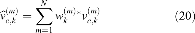
The estimate value of the state equation of the system by using the formulas (17) to (22), that is the result of output state estimate of optimization particle filtering. The estimate values of workboat position coordinates are calculated by the formulas (17) and (18), the estimate speed values in the X and Y directions are calculated by the formulas (19) and (20), and the estimate values of target point position coordinates are calculated by the formulas (21) and (22).

Step 8. Determine whether the maximum number of iterations is achieved

If the answer is right, exit the algorithm; else return to step 2.

Experimental results and discussion

Image processing experiment

Image collection

The image acquisition location is the crab farming base in Anfeng Town, Xinghua City, Jiangsu Province, China.

The simulation environment is as follows: CPU Intel Core2 Duo E7300 2.66 GHz, RAM 3.24GB, Intel ® G33/G31 ECF, MATLAB R2014a.

The image collection demand is as follows. Lens (China Shenzhen Jinghang Technology Co., Ltd.) is the megapixel industrial KBE-RT6200E/S lens. The focal length is 3.9–85.8 mm, and the view angle is −6°–54°. F1.6-C is the aperture parameter of the lens, and the aperture F is the ratio of lens’ focal length f to the diameter of the lens’ aperture D. We select C-type interface of the lens for this study. The surface size of image is 1/3, and the nearest distance is 0.15 m. The camera performs data transmission with the computer through USB2.0.

Image analysis

Floating aquatic plants generally exist in a variety of shapes in crab ponds. In this study, the aquatic plants present a striped distribution. In crab ponds, the collected aquatic images are generally affected by the diffuse reflection of water surface, especially when the light intensity is high. To reduce or eliminate the effect of surface reflection on the image acquisition quality, a polarizer is installed at the front of the camera, which can reduce the impact of water reflection on the collected images. Figures 4 and 5 show the comparison of images acquired with and without polarizer.⁴⁰

Figure 4.

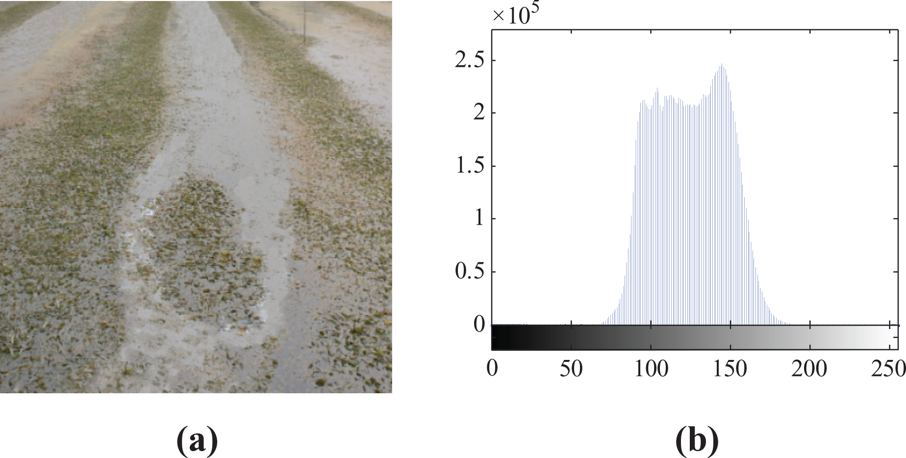
The original image and grayscale histogram without polarizer. (a) The original image and (b) grayscale histogram.

Figure 5.

The original image and grayscale histogram with polarizer. (a) The original image and (b) grayscale histogram.

From the visual perspective of Figures 4(a) and 5(a), the luminance of the original image collected after the installation of the polarizer is darken to some extent, and the brightness of the image is reduced. We can get the corresponding image histogram according to the original color image, as shown in Figures 4(b) and 5(b). The gray value of the corresponding histogram is also decreased to a great extent. We calculate the average gray value of the two images, we can get the gray value G ₁ = 126.71 of Figure 4(a) and the gray value G₂ = 109.32 of Figure 5(a), so the gray value is decreased by 13.72%. The comparison shows that the gray value of the image is reduced after the installation of the polarizer, the brightness of the image is also reduced to a certain extent, and the influence of the reflected light on the image quality can be reduced to a certain extent, which can reduce the difficulty of the image processing.

Image processing

In the visual system, the collected image information is used to segment the aquatic target, and the position of the aquatic area is determined. The straight line is fitted through the calculation of aquatic area, and then the visual navigation reference line is extracted. The main process of image processing is shown in Figure 6.

Figure 6.

The flow chart of image processing.

Navigation line extraction

In order to provide correct navigation information for the navigation system, the key is to use the image processing system to fit out the visual navigation baseline. Image segmentation is very important in image processing. In this study, we use the optimized pulse coupled neural network (PCNN) for image segmentation.^41,42 This method can not only optimize the weighted combination of PCNN maximum Shannon entropy and minimum cross entropy by particle swarm optimization (PSO) but also evaluate the optimization effect of parameters using the yield function, thus realizing the automatic optimization of network parameters and improving the operating efficiency and segmentation accuracy of PCNN.² For image de-noising, a 3 × 3 arithmetic mean filter window is used. In morphological treatment, a 1 × 3 template is used for expansion, and a 3 × 1 template is selected for corrosion.⁴³

In the process of extracting the navigation route, in order to reduce calculation time and memory usage of the Hough transform method, we choose to map the nonzero pixels in the binarized image to the accumulating units with large possibility rather than all accumulating units based on the traditional Hough transform algorithm, thus significantly reducing the computational complexity.^44,45 The image processing results are shown in Figure 7.

Figure 7.

Results of image processing: (a) grayscale, (b) de-noising image, (c) image segmentation, (d) morphological processing, (e) feature point extraction, and (f) extraction of navigation lines.

The experimental results are analyzed by the statistical analysis method. The image recognition accuracy rate γ is calculated by the following formula

γ = \frac{R}{N} \times 100 %

In the formula (26), R represents the number of images that can be correctly identified. N represents the total number of experiment collected images. We collected 60 images by the industrial camera. From the image processing experiment, it can be found that 49 images can accurately extract the navigation reference routes, and the recognition accuracy rate is 81.67%. Meanwhile, the average algorithm running time of an image is 653 ms. The accuracy rate and running time can meet the real-time and accuracy requirements for the automatic navigation system of aquatic plants-cleaning workboat.

Simulation experiment

In order to simulate the bearings-only tracking two-dimensional motion navigation model, the simulation of the state equation and measurement equation are shown in formulas (1) and (5). Three different navigation and positioning methods, that is, PF, GRNN-PF, and FOA-GRNN-PF, are used to conduct the comparative experiments by MATLAB R2014a.

The model parameters are set as follows: w(t) is the Gaussian system noise, which obeys the distribution of N(0, 0.1); v(t) is the observed noise, which obeys the distribution of N(0, 0.5); and X(0) = [5.5, 0.8, 3.5, 0.2] is the initial state. In the simulation experiment, we face more difficulty to get the true value of the initial moment, and we usually give the state value through the priori information, but there is usually a margin of error. In order to match the actual real value, we add a certain margin of random error on the basis of the real value and obtain the initial value of the state estimation. The size of the random error has a great influence on filtering performance in the front time, but PF has a certain feedback mechanism. The prediction error of the current moment will participate in the correction of the filtering result at the next moment, so the initial error has less influence on the filtering accuracy at a later moment. In this article, we set the initial time coordinate random error upper limit as 2.5 and the maximum random error rate as 0.1. The initial value range of the coordinate state is set to [−2, 2], and the initial value range of the velocity state is [−0.5, 0.5]. Finally, the particle swarm at the initial moment is obtained by the normal distribution. The root mean square error (RMSE) formula is as follows

RMSE = \sqrt{\frac{1}{T} \sum_{t = 1}^{T} {[θ_{(k t)} - \overset{\land}{θ_{(k t)}}]}^{2}}

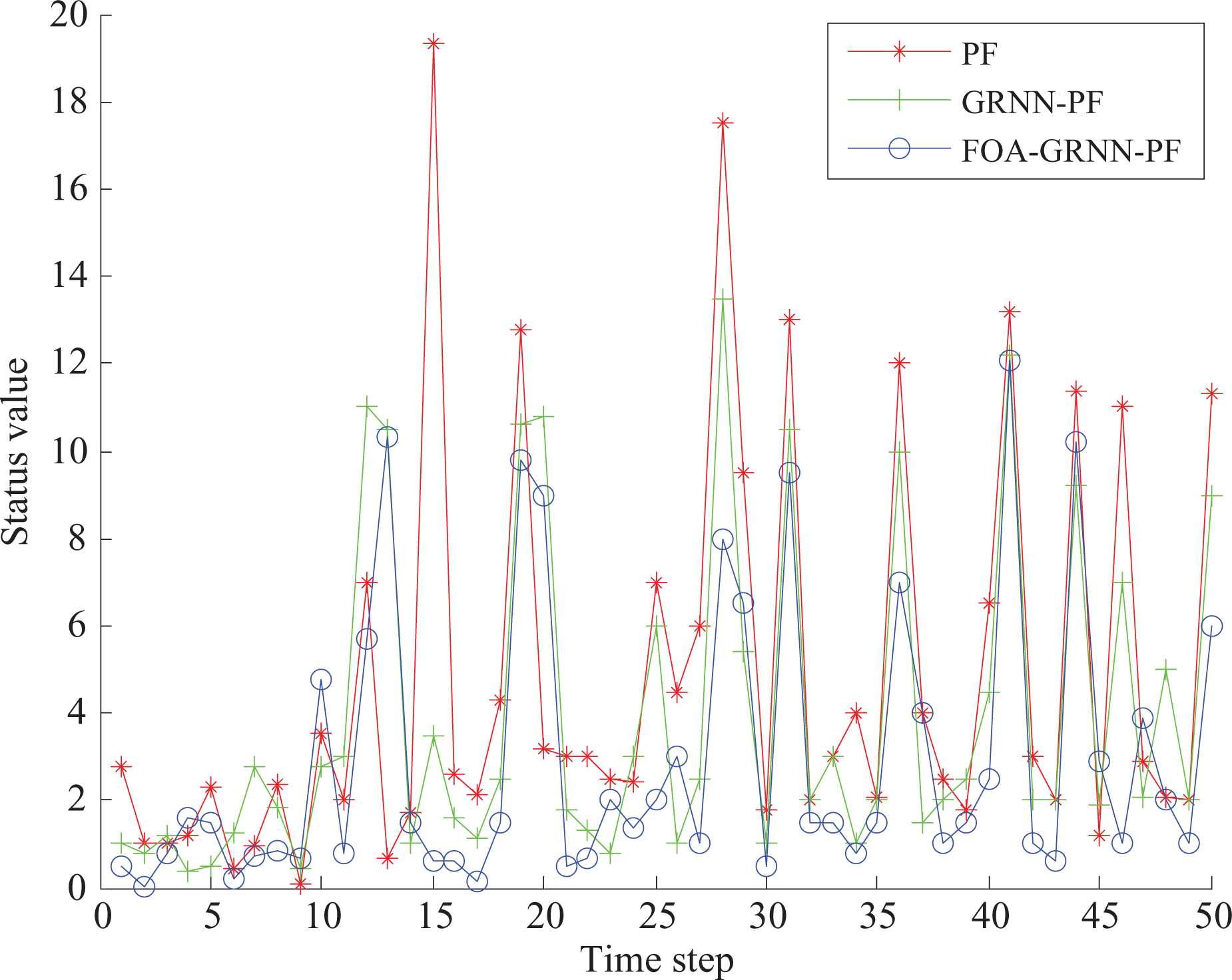
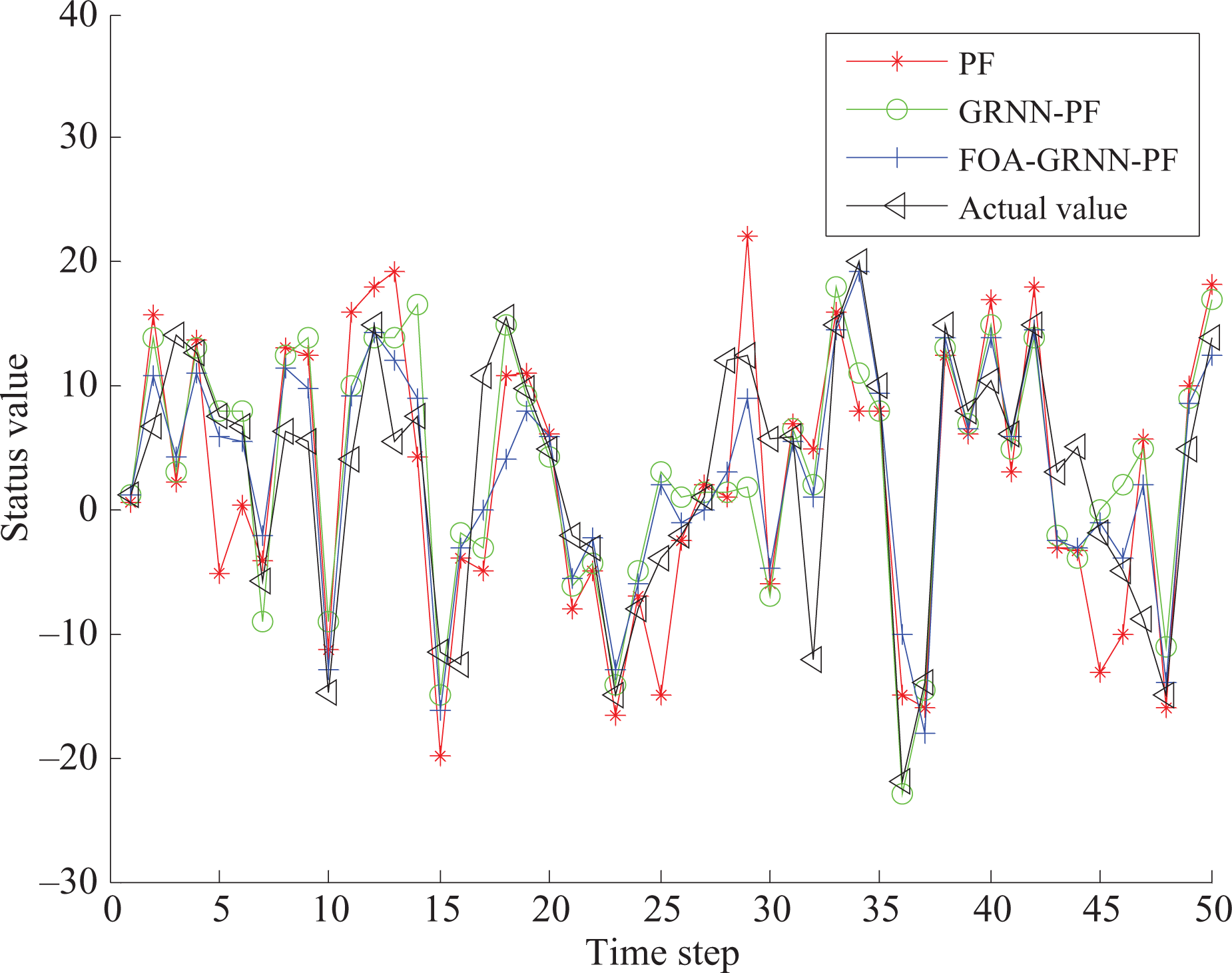
where θ_(kt) represents the measurement azimuth and $\overset{\land}{θ_{(k t)}}$ represents the estimated value of measurement azimuth.

For better testing the accuracy and efficiency of the proposed method, the numbers of the selected particles are set as N ₁ = 30, N ₂ = 60, and N ₃ = 100, respectively, and the sampling time step is set to 50 s. These experiments can be simulated separately to obtain the filter positioning status estimate and the absolute value of filter error. The results are shown in Figures 8 to 13.

Figure 8.

Status estimation of filter (N ₁ = 30).

Figure 9.

Absolute value of filter error (N ₁ = 30).

Figure 10.

Status estimation of filter (N ₂ = 60).

Figure 11.

Absolute value of filter error (N ₂ = 60).

Figure 12.

Status estimation of filter (N ₃ = 100).

Figure 13.

Absolute value of filter error (N ₃ = 100).

As can be seen in Figures 8 to 13, compared with the PF and GRNN-PF methods, the optimized σ value of GRNN can be obtained by FOA space optimization, and the particle state updating equation of PF can be further iterated by the optimized GRNN to improve the particle distribution.

The mean of RMSE and running time can be calculated from the simulation results of different particles filter methods and the number of particles. The results are shown in Table 1. From Table 1, the mean_R of RMSE of the FOA-GRNN-PF state values decreases by 12.39% and 6.87%, respectively, compared with those of PF and GRNN-PF. The mean_T of the running time decreases by 16.04% and 9.14%, respectively, compared with those of PF and GRNN-PF. It can be seen that the proposed method improves the accuracy of PF and the computational efficiency of the algorithm, which has certain advantages.

Table 1.

Experimental data of simulation.

Number of particles	RMSE			Number of particles	Running time (s)
Number of particles	PF	GRNN-PF	FOA-GRNN-PF	Number of particles	PF	GRNN-PF	FOA-GRNN-PF
30	7.1245	7.0346	6.3891	30	0.2143	0.2076	0.1679
60	7.3017	6.5354	6.3126	60	0.1810	0.1731	0.1595
100	9.1784	8.6378	7.9794	100	0.2687	0.2328	0.2301
Mean_R	7.8682	7.4026	6.8937	Mean_T	0.2213	0.2045	0.1858

RMSE: root mean square error; PF: particle filter; FOA: fruit fly optimization algorithm; GRNN: generalized regression neural network.

In theory, the running time of PF is approximately linear relation with the number of particles, that is, the more the number of particles, the longer the running time and the higher the precision. One of the purposes of this simulation experiment is to show that the proposed method can achieve the desired precision using fewer particles. By further analysis of Table 1, it can be found that the estimation accuracy results are close to each other when the numbers of particles are 30 and 60, which are better than the experimental results when the number of particles is 100. This also demonstrates that the proposed method can use fewer particles to achieve the required accuracy, and thus reduce the running time of algorithm.

In summary, through the simulation experiment, it can be obtained that the proposed method has advantages in operational accuracy and efficiency compared with PF and GRNN methods. In addition, the FOA-GRNN-PF method can achieve the required precision and efficiency in the fewer number of particles, therefore it has a higher comprehensive performance.

Navigation experiment and result analysis

Experimental object

Figure 14 illustrates the structure of aquatic plants-cleaning workboat in the navigation experiment. The workboat is mainly composed of a hull, two wheel propellers, the GPS sensor module, a cutting conveyor, a cutting depth regulator, the aquatic plants paving device, and other devices.

Figure 14.

Structure diagram of the workboat.

The digital photo of aquatic plants cleaning workboat is shown in Figure 15. The workboat has three working modes, including remote control, manual navigation, and autonomous navigation. It adopts the design of a single hull. The positive and negative wheels are installed on both sides of the hull as the power devices to achieve a spot turn of 360° of the workboat. The main controller uses 32-bit processor S3C2440A based on ARM920T from SAMSUNG Electronics Company (Giheung-Eup Yongin-City, Gyeonggi-Do, Korea), and is configured with the Linux operating system LCD can display battery power information and other information as well as user operation interfaces such as electronic map navigation interface, and navigation trajectory can also be scheduled on it. All devices of the system are driven by a 48 V lithium battery with a capacity of 120 AH. In order to get the navigation point information of the workboat system in real time, GPS navigation module used the BD982 model, and the navigation device is developed by the United States Trimble navigation company. Lens is the megapixel industrial KBE-RT6200E/S device which is developed by China Shenzhen Jinghang Technology Co., Ltd.

Figure 15.

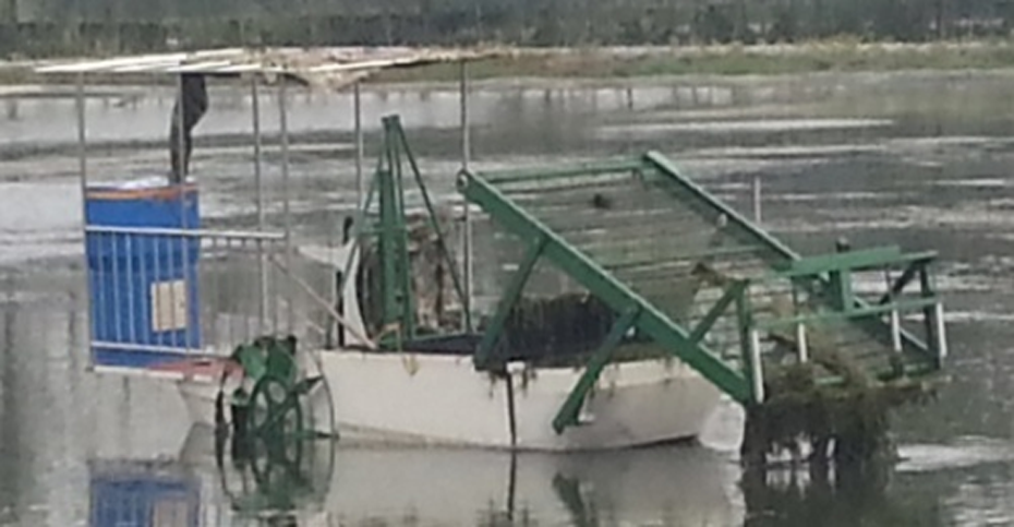
Digital photo of the aquatic plants cleaning workboat.

Navigation experiment design

According to the distribution characteristics of aquatic plants in crab ponds, the geographic information system can provide the latitude and longitude coordinates of pond water. The target waypoints, that is, the preset route, are set in the system interface. The system then uses the image detection visual navigation line to judge whether there are aquatic plants in the vicinity of the workboat and further chooses the navigation method according to the results of image detection. If there is no visual navigation route from image detection, it uses the GPS navigation; if there is visual navigation line, it uses the visual navigation. In the design process, the visual coordinates in the visual information need to be transformed into the earth coordinates, and the coordinate system must be unified. The position information in the unified coordinates is optimized by the proposed method to obtain the new position coordinates.

Navigation experiment

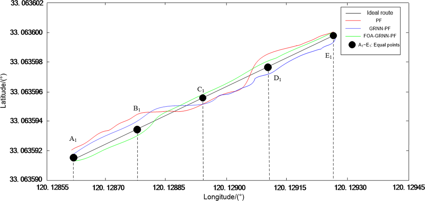
In order to further verify the method proposed in this study, we also use those above three methods in the simulation experiment to repeat the navigation experiment. The experiment site is selected from the crab farming base of Anfeng Town, Xinghua City, Jiangsu Province, China. Through the navigation experiment, we can get the corresponding latitude and longitude coordinates. Since the workboat sails on the water surface, the skyward direction is not taken into account in this study and the navigation route follows a two-dimensional trajectory. The latitude and longitude coordinates of the starting and ending points of the boundary for aquatic plants can be obtained manually by GPS. In crab ponds, the shape of floating aquatic plants is considered as a striped one, so the connection line between the starting and ending points can be approximated as the ideal route. To compare the visual effects with the objective data from the route, two groups of representative navigation experiment routes are selected for analysis, and the results are shown in Figures 16 and 17.

Figure 16.

Navigation experiment (1).

Figure 17.

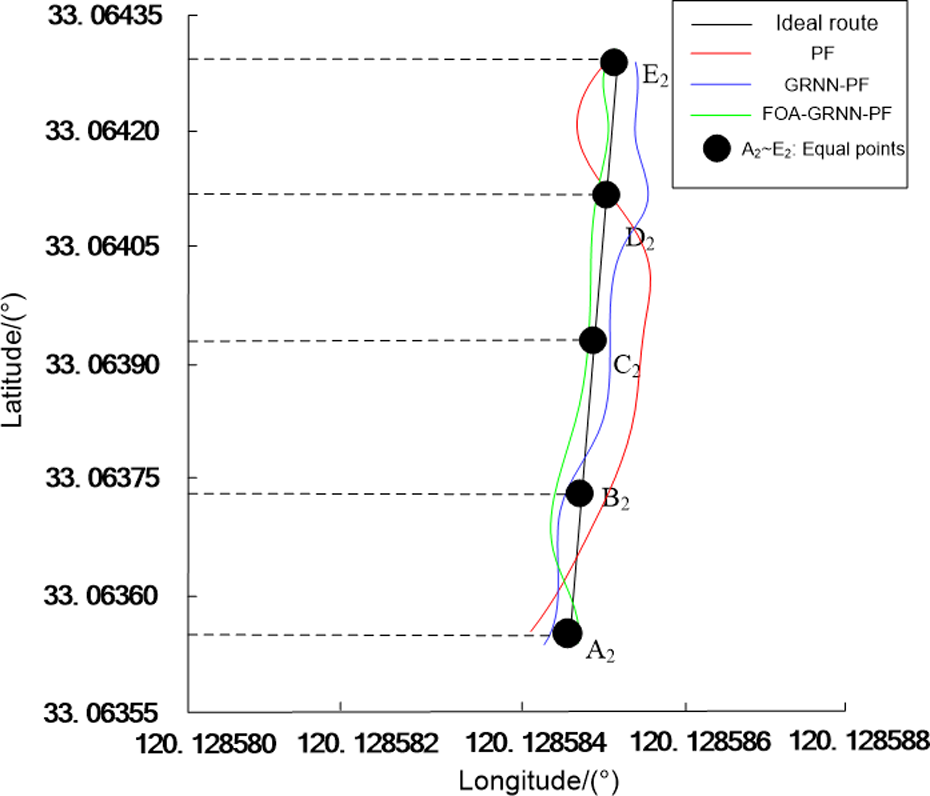
Navigation experiment (2).

These two groups of experiments are conducted in two different crab ponds. The crab area for navigation experiment (1) is about 28 acres, and the workboat sailing distance is about 85.12 m, with a sailing speed of 0.48 m/s. The crab area for navigation experiment (2) is about 20 acres, and the workboat sailing distance is about 58.36 m, with a sailing speed of 0.56 m/s. Because the width ranges of latitude and longitude coordinates are quite different, the corresponding coordinate unit scale is reduced when the navigation maps are drawn. The unit scale of latitude coordinate is narrowed to get Figure 16, and that of longitude is narrowed to get Figure 17. In order to evaluate the positioning effect of the three navigation methods relative to the objective data, five equal points (including the starting and ending points) are selected as the target points on the ideal route. The line connecting the black points is the ideal navigation route, and the red, blue, and green solid lines represent the navigation routes of PF, GRNN-PF, and FOA-GRNN-PF, respectively.

According to the visual effects of the route coordinates in Figures 16 and 17, PF, GRNN-PF, and FOA-GRNN-PF can all complete the navigation experiment. However, the distance between the trajectory route of the PF location method and the ideal route is the largest, and PF has the worst cleaning effect on the aquatic plants. GRNN-PF has passable navigation and positioning effect, but its cleaning effect on the aquatic plants needs to be improved. The FOA-GRNN-PF method has the best navigation and positioning effect, and the distance between the trajectory route and the ideal route is the smallest. Its navigation route is the closest to the ideal route, and the best cleaning effect on the aquatic plants can be achieved.

Result analysis

In Figure 16, A ₁–E ₁ are equal points that are used as the target position. We can get the actual route through all these three navigation experiment methods, and the actual latitude and longitude coordinates can be read through GPS. On one hand, there are some differences in the navigation path and navigation time between any two equal points for the three methods. On the other hand, according to Figure 16, the workboat sails roughly along the longitude direction, and the longitude coordinate varies rapidly as the workboat sails. Therefore, it is difficult to compare the positioning error of the three methods by the longitude error for the navigation experiment (1). In view of this, we choose the latitude error as the calculation object. In the three navigation methods, the longitude value of the equal point is used as the reference, and the latitude value of each method can be obtained as the measured latitude value. The measured latitude value minus the target latitude value is the latitude error. The measured latitude values and latitude errors of the three methods are given in Table 2.

Table 2.

Measured latitude values and error values (º).

Position	Measured latitude values				Absolute error (×10⁻⁸)
Position	Target position	PF	GRNN-PF	FOA-GRNN-PF	PF	GRNN-PF	FOA-GRNN-PF
A ₁	33.06359115	33.06359238	33.06359203	33.06359024	123	88	91
B ₁	33.06359373	33.06359451	33.06359475	33.06359324	78	102	49
C ₁	33.06359631	33.06359562	33.06359568	33.06359684	69	63	53
D ₁	33.06359889	33.0635997	33.06359832	33.06359951	81	57	62
E ₁	33.06360147	33.06360203	33.06360104	33.06360202	56	43	55
Mean	33.06359631	33.06359685	33.06359636	33.06359637	81	71	62

PF: particle filter; FOA: fruit fly optimization algorithm; GRNN: generalized regression neural network.

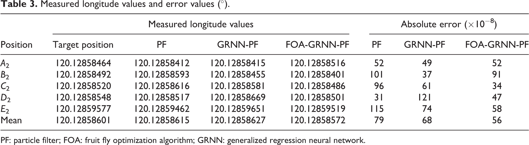
In Figure 17, A ₂–E ₂ are equal points that are used as the target position. For the selected navigation experiment (2), the workboat generally sails along the latitude direction, and the latitude coordinate varies rapidly as the workboat sails. Therefore, it is difficult to compare the positioning error of the three methods by the latitude error. In view of this, we choose the longitude error as the calculation object. The measured longitude value subtracts the target longitude as the longitude error. The measured longitude values and longitude errors of the three methods are given in Table 3.

Table 3.

Measured longitude values and error values (º).

Position	Measured longitude values				Absolute error (×10⁻⁸)
Position	Target position	PF	GRNN-PF	FOA-GRNN-PF	PF	GRNN-PF	FOA-GRNN-PF
A ₂	120.12858464	120.12858412	120.12858415	120.12858516	52	49	52
B ₂	120.12858492	120.12858593	120.12858455	120.12858401	101	37	91
C ₂	120.12858520	120.12858616	120.12858581	120.12858486	96	61	34
D ₂	120.12858548	120.12858517	120.12858669	120.12858501	31	121	47
E ₂	120.12859577	120.12859462	120.12859651	120.12859519	115	74	58
Mean	120.12858601	120.12858615	120.12858627	120.12858572	79	68	56

PF: particle filter; FOA: fruit fly optimization algorithm; GRNN: generalized regression neural network.

It can be seen from Table 2, with the ideal target position as the reference, PF has the largest latitude error while FOA-GRNN-PF has the smallest. Compared with those of PF and GRNN-PF, the latitude error of FOA-GRNN-PF decreases by 23.45% and 12.68%, respectively. Similarly, according to Table 3, the longitude error of FOA-GRNN-PF decreases by 29.11% and 17.65%, respectively, compared with those of PF and GRNN-PF.

To further compare the positioning effect of these three methods, the distance error is calculated. The length of the vertical line segment between the actual position coordinate point and the ideal path is defined as the distance error d, which can be obtained by the following method.

In Figure 18, the position information can be directly read according to the latitude and longitude coordinates of GPS. P(x ₁,y ₁) is the current position of the workboat, and A(x ₂,y ₂) and E(x ₃,y ₃) are the starting and ending points of the target route. Q(x ₄,y ₄) is the vertical projection point of P on the AE line. Among them, x_i (i = 1 to 4) is the longitude coordinate of each position, y_i (i = 1 to 4) is the latitude coordinate of each position, the unit is degree. In addition, the direction of the waterway is A→E, d is the distance error.

Figure 18.

Schematic of the distance error.

Once the hull deviates from the waterway, one can draw a line from point P along the direction perpendicular to the route AE, which intersects with the route AE at the point Q(x₄,y₄). Then the coordinates of Q can be derived according to formulas (28) and (29) that describe the perpendicular distance from a point to a line.

x_{4} = \frac{(y_{1} - y_{2}) [x_{1} (y_{3} - y_{2}) + x_{2} (y_{1} - y_{3})] + y_{3} {(x_{1} - x_{2})}^{2}}{{(x_{2} - x_{3})}^{2} + {(y_{2} - y_{3})}^{2}}

y_{4} = \frac{(x_{1} - x_{2}) [y_{2} (x_{1} - x_{3}) - y_{1} (x_{2} - x_{3})] + y_{3} {(y_{1} - y_{2})}^{2}}{{(x_{2} - x_{3})}^{2} + {(y_{2} - y_{3})}^{2}}

Considering the spherical coordinate plane, it is more accurate through calculating the haversine distance error as the distance error. Thus, the distance between the points P and Q can be derived through the formula of computing the distance between two points based on longitudinal and latitudinal coordinates:

d = 2 \cdot R \cdot arcsin {\sqrt{{sin}^{2} [\frac{(y_{1} - y_{4}) π}{360}] + cos (\frac{y_{1} \cdot π}{180}) \cdot cos (\frac{y_{4} \cdot π}{180}) \cdot {sin}^{2} [\frac{(x_{1} - x_{4}) π}{360}]}}

where R = 6,378,137 m is the radius of the earth, and the unit of d is m.

The calculated distance d is the distance error. Using the above method, we can obtain the distance error curves of the three navigation methods respectively. The results for navigation (1) and (2) experiments are shown in Figure 19(a) and (b), respectively.

Figure 19.

Distance error curves of PF, GRNN-PF, and FOA-GRNN-PF. (a) Navigation experiment (1) and (b) navigation experiment (2). PF: particle filter; FOA: fruit fly optimization algorithm; GRNN: generalized regression neural network.

According to the experimental results, the distance error of PF is the largest, followed by that of GRNN-PF, and that of the proposed method is the smallest. From the perspectives of navigation time and work efficiency, the PF method has relatively longer actual route distance and its working time is the longest, which means the lowest working efficiency. In contrast, the proposed method has the shortest actual route distance due to its smallest distance error, and its working time is the shortest, which means the highest working efficiency.

Through the above simulation and navigation experiments, it can be concluded that the navigation accuracy of the proposed navigation filtering method can be further improved compared with that of PF and GRNN-PF; meanwhile, the RMSE of the proposed method is reduced. These results confirm that the proposed FOA-GRNN-PF method has certain practicability and feasibility.

Conclusions and future work

The smoothing factor σ of transfer function for the GRNN model layer is obtained by FOA space optimization, which can improve the global optimization ability of particles by iterating the particle state updating equation through the optimized GRNN. The new method can avoid particle dilution and keep its diversity. Compared with those of PF and GRNN-PF, the RMSE of FOA-GRNN-PF state values decreases by 12.39% and 6.87%, respectively, and the running time decreases by 16.04% and 9.14%, respectively.

Through repeated navigation experiments for the aquatic plants-cleaning workboat in the river crab ponds, it is found that the latitude error of the proposed method decreases by 23.45% and 12.68%, respectively, and that the longitude error decreases by 29.11% and 17.65%, respectively, compared with those of PF and GRNN-PF.

The proposed method has further improved the positioning accuracy of the aquatic plants-cleaning workboat. It has certain practicability and feasibility, and can improve the level of accurate operation in cleaning aquatic plants of crab farming in China.

Image processing technology is the key technology in our navigation positioning system. In this study, we only focus on the image processing system where the aquatic plants present a striped distribution in the sunny weather with good lighting conditions. In fact, it is a complex problem to investigate the image processing system with different lighting conditions, weather conditions, and water ripples, and further efforts should be made on this issue in the future.

The proposed method in this article is applied to aquatic plants-cleaning workboat in crab farming. It is of great significance to improve the navigation and positioning accuracy and work efficiency of the workboat. In the future work, through combining with the method model, the proposed method can be used in other agricultural robots, such as unmanned rice transplanter, weeding robot, and so on. It can also be used in the navigation and positioning study of other industrial robots, such as underwater robot, automated guided vehicle, and so on.

Footnotes

Declaration of conflicting interests

The authors declared no potential conflicts of interest with respect to the research, authorship, and/or publication of this article.

Funding

The authors disclosed receipt of the following financial support for the research, authorship, and/or publication of this article: This work is supported by the National Natural Science Foundation of China (no. 31571571); Natural Science Foundation of Fujian Province (no. 2018J01471); Priority Academic Program Development of Jiangsu Higher Education Institutions (PAPD); Ordinary University Graduate Student Research Innovation Projects of Jiangsu Province (no. KYLX15_1075); Natural Science Foundation of Jiangsu Province (no. BK20170536); The Key R&D Project (Modern Agriculture) of Jiangsu Province (no. BE2017331); Jiangsu Province Ocean and Fishery Technology I&P Project (no. Y2017-36); The College Student Innovative Training Project of Fujian Province (no. 201710397047). The Science and Technology Project of Fujian Province Education Department (no. JAT160506); and The Science and Research Fund of Wuyi University (no. 201504).

ORCID iD

Chengzhi Ruan

References

Sun

Zhao

Hong

. Design of automatic and uniform feeding system carried by workboat and effect test for raising river crab. Trans Chin Soc Agric Eng 2015; 31(11): 31–39.

Ruan

Zhao

. Aquatic plants image segmentation based on PSO-PCNN in crab farming. Int Agric Eng J 2017; 26(1): 199–211.

Shang

. Design on 9GSCC-1.4H type submerged plants harvesting boat. Trans Chin Soc Agric Mach 2006; 37(1): 59–62.

Liu

Zhao

Sun

. Control system for automatic aquatic plant cleaning ship. Trans Chin Soc Agric Mach 2014; 45(S1): 281–286.

Ruan

Zhao

Liu

. Integrated navigation positioning method based on IPSO-UKF for aquatic plants cleaning workboat. Trans Chin Soc Agric Mach 2017; 48(7): 38–45.

Ruan

Zhao

Sun

. Design and testing of a control system associated with the automatic feeding boat for farming Chinese river crabs. Comput Electron Agric 2018; 150: 14–25.

Jaldehag

Johansson

Davis

. Geodesy using the Swedish permanent GPS network: effects of snow accumulation on estimates of site positions. Geophys Res Lett 2013; 23(13): 1601–1604.

Gui

Wang

. A review of visual inertial odometry from filtering and optimisation perspectives. Adv Robot 2015; 29(20): 1289–1301.

Meng

Zhang

Qiu

. Navigation line detection for farm machinery based on improved genetic algorithm. Trans Chin Soc Agric Mach 2014; 45(10): 39–46.

10.

Jiao

Jiang

. Crop rows detection based on parallel characteristic of crop rows using visual navigation. Trans Chin Soc Agric Eng 2009; 25(12): 107–113.

11.

Güzel

. Autonomous vehicle navigation using vision and mapless strategies: a survey. Adv Mech Eng 2013; 234747: 1–10.

12.

Yang

Scherer

. Multi-camera visual SLAM for autonomous navigation of micro aerial vehicles. Robot Auton Syst 2017; 93: 116–133.

13.

Ristic

Arulampalam

Gordon

. Beyond the kalman filter-particle filters for tracking applications. IEEE Trans Aeros Elect Syst 2003; 19(7): 37–38.

14.

Sun

Tang

. Improved particle filter algorithm for INS/GPS integrated navigation system. Control Theory Appl 2010; 34(4): 2392–2396.

15.

Zhang

Liu

. Positioning method of vehicle navigation system based on improved particle filter. Trans Chin Soc Agric Eng 2011; 27(8): 227–231.

16.

Ahmed

Rutten

Bessell

. Detection and tracking using particle-filter-based wireless sensor networks. IEEE Trans Mobile Comput 2010; 9(9): 1332–1345.

17.

Yin

Zhu

. Intelligent particle filter and its application to fault detection of nonlinear system. IEEE Trans Ind Electron 2015; 62(6): 3852–3861.

18.

Gordon

Salmond

Smith

AFM

. Novel approach to nonlinear/non-Gaussian Bayesian state estimation. IEE Proc F - Radar Signal Process 1993; 140(2): 107–113.

19.

Torma

Szepesvári

. Local importance sampling: a novel technique to enhance particle filtering. J Multi 2006; 1(1): 32–43.

20.

Zhao

. A fast Quasi-Monte Carlo-based particle filter algorithm. Acta Autom Sin 2010; 36(9): 1351–1356.

21.

Guo

Wang

. Quasi-Monte Carlo filtering in nonlinear dynamic systems. IEEE Trans Signal Process 2006; 54(6): 2087–2098.

22.

Talantzis

. An acoustic source localization and tracking framework using particle filtering and information theory. IEEE Trans Audio Speech Lang Process 2010; 18(7): 1806–1817.

23.

Zhong

Hopgood

. Particle filtering for TDOA based acoustic source tracking: nonconcurrent multiple talkers. Signal Process 2014; 96(5): 382–394.

24.

Hlinka

Hlawatsch

Djuric

. Distributed particle filtering in agent networks: a survey, classification, and comparison. IEEE Signal Process Magaz 2012; 30(1): 61–81.

25.

Yang

. Firefly algorithm, stochastic test functions and design optimisation. Int J Bio Inspir Comput 2010; 2(2): 78–84.

26.

Tian

Chen

. Firefly algorithm intelligence optimized particle filter. Acta Autom Sin 2016; 42(1): 89–97.

27.

Chen

Tian

. Intelligent particle filter based on bat algorithm. Acta Phys Sin 2017; 66(5): 1–10.

28.

Tyan

Kim

. Convolutional neural network with particle filter approach for visual tracking. KSII Trans Int Inform Syst 2018; 12(2): 693–709.

29.

Chen

. Quasi-Monte Carlo particle filter algorithm for target tracking based on GRNN. Inform Control 2012; 41(6): 760–773.

30.

Pan

. A new fruit fly optimization algorithm: taking the financial distress model as an example. Know Base Syst 2012; 26(2): 69–74.

31.

Guo

. A hybrid annual power load forecasting model based on generalized regression neural network with fruit fly optimization algorithm. Know Base Syst 2013; 37(2): 378–387.

32.

Carpenter

Clifford

Fearnhead

. Improved particle filter for nonlinear problems. IEEE Proc Radar Sonar Navig 1999; 146(1): 2–7.

33.

Yap

Lim

Abidin

. A hybrid ART-GRNN online learning neural network with a ε-insensitive loss function. IEEE Trans Neural Netw 2008; 19(9): 1641–1646.

34.

Gustafsson

. Particle filter theory and practice with positioning applications. IEEE Aerosp Electron Syst Magaz 2010; 25(7): 53–82.

35.

Goodall

Kadirkamanathan

. Estimation of parameters in a linear state space model using a Rao-Blackwellised particle filter. IEE Proc Control Theory Appl 2004; 151(6): 727–738.

36.

Koval

Pollard

Srinivasa

. Pose estimation for planar contact manipulation with manifold particle filters. Int J Robot Res 2015; 34(7): 4541–4548.

37.

Pan

. Using fruit fly optimization algorithm optimized general regression neural network to construct the operating performance of enterprises model. J Taiyuan Univ Technol 2011; 29(4): 1–5.

38.

Lin

. Analysis of service satisfaction in web auction logistics service using a combination of fruit fly optimization algorithm and general regression neural network. Neural Comput Appl 2013; 22(3–4): 783–791.

39.

Mousavi

Alikar

Niaki

STA

. An improved fruit fly optimization algorithm to solve the homogeneous fuzzy series–parallel redundancy allocation problem under discount strategies. Soft Comput 2016; 20(6): 2281–2307.

40.

Sasagawa

Shishido

Ando

. Image sensor pixel with on-chip high extinction ratio polarizer based on 65-nm standard CMOS technology. Opt Express 2013; 21(9): 11132–11140.

41.

Wang

Cheng

. Review of pulse-coupled neural networks. Image Vis Comput 2010; 28(1): 5–13.

42.

Kuntimad

Ranganath

. Perfect image segmentation using pulse coupled neural networks. IEEE Trans Neural Netw 1994; 2(3): 591–598.

43.

Bang

Piao

. Noise reduction in digital hologram using wavelet transforms and smooth filter for three-dimensional display. IEEE Photonics J 2013; 5(3): 6800414.

44.

Oja

Kultanen

. A new curve detection method: randomized Hough transform (RHT). Pattern Recognit Lett 1990; 11(5): 331–338.

45.

Walsh

Raftery

. Accurate and efficient curve detection in images: the importance sampling Hough transform. Pattern Recognit 2002; 35(7): 1421–1431.

A new optimization particle filtering navigation location method for aquatic plants cleaning workboat in crab farming

Abstract

Keywords

Introduction

Materials and methods

System model

State equation

Measurement equation

Principles of FOA-GNRR-PF

Basic principles of PF

Step 1. Sampling

Step 2. Normalized weight calculation

Step 3. Re-sampling

Step 4. Estimate of output state

FOA-GRNN network structure

Procedure of the FOA-GRNN-PF algorithm

Step 1. Particle sample initialization

Step 2. Calculate the importance of the weight of each particle

Step 3. Optimize GRNN parameters according to FOA

Step 4. Optimize PF by GRNN and use GRNN to calculate the weights of the offspring particles

Step 5. Normalize the weights of all particles

Step 6. Resampling techniques are applied to get a new set of particles

Step 7. System output

Step 8. Determine whether the maximum number of iterations is achieved

Experimental results and discussion

Image processing experiment

Image collection

Image analysis

Image processing

Navigation line extraction

Simulation experiment

Navigation experiment and result analysis

Experimental object

Navigation experiment design

Navigation experiment

Result analysis

Conclusions and future work

Footnotes

Declaration of conflicting interests

Funding

ORCID iD

References