Sage Journals: Discover world-class research

Abstract

To improve the modeling accuracy and efficiency of the tool wear monitoring system, a generalized regression neural network is adopted to build the tool wear prediction model because its excellent performance on learning speed and fast convergence to the optimal results whether the sample data are small or large. The low predictive accuracy and efficiency are caused by traditionally manual adjustment of the spread parameters in generalized regression neural network and then the improved fruit fly optimization algorithm is proposed to optimize the spread parameters of regression neural network automatically. Combining the improved fruit fly optimization and generalized regression neural network, the tool wear prediction method is proposed in the paper. Various experiments are carried out to validate the proposed method and the comparison results show a good agreement. In addition, the proposed method is compared to the tool wear prediction method in the literature, and the comparison results also show that the proposed method can achieve better performance.

Keywords

Tool wear monitoring generalized regression neural network improved fruit fly optimization algorithm particle swarm optimization

Introduction

Tool wear condition plays an important role in the machined surface quality and machine reliability during metal cutting,¹ as tool wear is inevitable, and has great influence on the cutting forces and temperature, which will affect the surface roughness and residual stresses.² Abundant research shows that tool condition monitoring not only can improve the tool utilization rate, but also avoid errors caused by damage of tool scrap.³ Therefore, a tool wear monitoring system with useful information being extracted from the measured signals is necessary for industry to maintain the desired machining requirement. Usually, the core requirement of a tool wear monitoring system is analysis of the measured signal to determine the tool wear condition. In terms of the approaches to acquire the signals, tool wear monitoring system could be generally categorized into direct methods and indirect methods.⁴ Direct methods include optical, radioactive, and electrical approaches, which focus on the direct measurement of the tool wear, while the indirect methods aim at measuring related parameters, such as cutting forces, vibrations, temperature, to “predict” the tool wear.

Among direct methods, optical measurement is the mainstream. Aiming at monitoring the flank wear, Cakan⁵ taps a photo sensor to detect the diameter change of workpiece. Barreiro et al.⁶ use image analysis technique to derive a geometrical descriptor; industrial high-speed cameras-based systems were also proposed to monitor tool wear.^7–9 Although the direct methods have high accuracy, they also cause interruptions of manufacturing process, which lead to lack of convenience and the on-line monitoring capability.

In contrast, indirect methods could estimate the tool wear by analyzing the relevant parameters without cutting off the manufacturing process. In the last few years, researchers focused on finding the law between tool wear and process parameters, as they are believed to contribute to the derivation of tool wear. For example, as a result of different wear modes, the cutting force needed to remove the material of workpiece increases gradually and the rubbing between the chip and workpiece against the tool produce vibration thus cutting force and vibration are believed to be the crucial features and are widely concerned by researchers^10,11 for their established theory. Other parameters, such as the temperature, spindle power/current, and emitted sound, also play roles in tool wear. Furthermore, cutting conditions, such as cutting speed, cutting depth, and feed rate, are also quite important since they could be coupled into signals like cutting force, vibrations, and so on. More often than not, it is hard to predict the tool wear only based on one or two features mentioned above; thus, sensor fusion model was widely concerned and adopted to establish the monitoring system.

Artificial intelligence technology, including the neural network, the support vector machine, and the generative adversarial network, has become so popular these years and machine learning methods have been wildly applied to many fields, for instance, memristor-based multilayer neural networks for pattern recognition,¹² memristor-based echo state network for time-series forecasting,¹³ and generative adversarial neural networks for video generation.¹⁴ Artificial intelligence technology is used to establish the black-box model between input variables and output variables. Machine learning methods are also widely applied to predict the tool wear/life using multiple input features. PS Paul and AS Varadarajan¹⁵ use back-propagation (BP) neural network to predict tool lives and failure modes for experiments not used in training, which showed a satisfying precision. But BP neural network has its own weaknesses. It would easily fall into a local optimum and is slow in convergence and weak in generalization ability. Shi and Gindy¹⁶ use multiple sensors to extract features from manufacturing process and establish a least squares support vector machine–based model to predict the broaching tool wear. But it has a high computational complexity which need more calculating time. In this article, the general regression neural network (GRNN), a kind of memory-based neural network and effective regression method proposed by Specht,¹⁷ is adopted to build the prediction model due to its dynamic learning characteristic, straightforward internal structure, and high fault tolerance ability. The GRNN has excellent performances on approximation ability and learning speed, and it is fast learning and convergence to the optimal regression surface as the number of sample data becomes very large. When the number of sample data is small, the GRNN still has a good forecasting result.¹⁸ However, the shortcoming of applying the GRNN model is that it is very difficult to select the spread parameter properly. Polat and Yıldırım¹⁹ use genetic algorithm to optimize the spread parameter of the GRNN for pattern recognition, and this optimized GRNN can provide higher recognition ability compared with the unoptimized GRNN.

Recently, a kind of drosophila inspired optimization algorithm has been developed, called fruit fly optimization algorithm (FOA),²⁰ which is a novel evolutionary computation and optimization technique. The FOA is a new approach for finding global optimization based on the swarm behavior of fruit fly. The main inspiration of FOA is that the fruit fly itself is superior to other species in sensing and perception. The FOA technique has the advantages of being easy to understand and to be written into program code which is not too long compared with genetic algorithm and particle swarm optimization (PSO) algorithm. Meanwhile, the PSO method may fall into local optimum easily which results in a low-precision forecast, as it is difficult to select parameters to solve different discrete and combinatorial optimization problems. Although the FOA method has shown its merit in many optimization problems, it still has some insufficiency. In the original optimization process, once the optimal individual is found, all the files will fly to that direction and find the next optimum through the random value in distance equation. Therefore, it will reduce the diversity of the population and the optimum individual may not be the global optimum. If the random value is not set appropriately, it will trap the flies in the local optimum, reducing the convergence precision and the speed of convergence. To resolve this problem, this article proposes an improved fruit fly optimization algorithm (IFOA) by introducing escaping parameter and control parameter. Therefore, this article uses the IFOA to automatically select the spread parameter value of the GRNN for improving the GRNN’s forecasting accuracy in predicting the tool wear/life.

In this article, the GRNN was adopted to build the prediction model and its spread parameter was optimized by the IFOA. The rest of this article is organized as follows: the GRNN model and the theory of IFOA are introduced in section “Introduction.” Section “IFOA-GRNN-based tool wear prediction model ” gives the detail settings of the prediction model. Section “Model setting ” proposes the evaluation criteria used to evaluate the prediction model. Section “Case study” makes two case study to verify the ability of the proposed prediction model and ultimately, section “Conclusion” concludes this article.

IFOA-GRNN-based tool wear prediction model

The output of GRNN is calculated according to the Parzen window estimation.²¹ Considering independent variable x and its function y are both random variables, assume the X is a real measured value of the random variable x and then, the conditional mean of y of the given X could be presented as

\hat{Y} = E (y | X) = \frac{\int_{- \infty}^{\infty} yf (X, y) dy}{\int_{- \infty}^{\infty} f (X, y) dy}

(1)

Assuming the $f (x, y)$ is contributed to the normal distribution, equation (1) could then be

\hat{Y} = \frac{\sum_{i = 1}^{n} Y_{i} \exp [- \frac{{(X - X_{i})}^{T} (X - X_{i})}{2 σ^{2}}]}{\sum_{i = 1}^{n} \exp [- \frac{{(X - X_{i})}^{T} (X - X_{i})}{2 σ^{2}}]}

(2)

The GRNN is totally consisted of four layers;²² each layer consists of one or more neurons. For example, taking the depth of cut, cutting speed, feed rate, and cutting time as the inputs, a GRNN-based tool wear prediction model is shown in Figure 1.

Figure 1.

The architecture of GRNN.

Therefore, the GRNN model has only one parameter $σ$ that needs to be determined, which is very important in using GRNN for forecasting. The spread parameter $σ$ determines how closely the network approximates the sample data; however, there are few empirical methods to choose the spread parameter $σ$ . It is often obtained by manual adjustment or using the hold out method, which is lack of efficiency and accuracy, especially when the sample becomes very large, it will take numerous computing time. Therefore, we should develop an automatically efficiently method for selecting the appropriate spread parameter in the GRNN model. Meanwhile, based on the principles of the GRNN, another effective form of Parzen window called city block distance metric is also adopted, which is the sum of the absolute difference between the pattern and the input vector in all dimensions.¹⁹

The spread parameter in GRNN model can be selected by optimization search algorithms, such as PSO and genetic algorithm, but in this article, we developed an IFOA to select the optimal spread parameter. The basic FOA is a novel evolutionary algorithm to find the global optimization based on the forage behavior of the fruit fly.^23,24 This kind of forage behavior is able to gradually approach the food source until the expectation is achieved by the acute vision and the gathered smell information through companions. The iteration of the process to find the food is shown in Figure 2. Compared to PSO, it is much easier to implement for programming and understanding. However, in the original optimization process, once the optimal individual is found, all the files will fly to that direction and find the next optimum through the random value in distance equation. This reduces the diversity of the population and the optimum individual may not be the global optimum. If the random value was not set appropriately, it will trap the flies in the local optimum, reducing the convergence precision and the speed of convergence. To resolve this problem, escaping parameter and control parameter are proposed to improve the original FOA in this article, in which escaping parameter can make population search beyond the optimum individual and the control parameter can increase the diversity of searching direction. The IFOA is used to select the appropriate spread parameter in the GRNN model and city block distance metric. It has the advantages of FOA and can avoid falling into local optimum.

Figure 2.

Food researching process of fruit flies.

Compared with the SFOA-GRNN model proposed by R Hu et al.,²⁵ we developed control parameter to increase the diversity of search direction of each population according to individual optimum by appropriately increasing the step size and escaping parameter to avoid the smell concentration S(i) attracting global population, which can cause falling into local optimum. The steps of the IFOA-GRNN model could be concluded as follows (each step is presented as pseudo-code):

Step 1: Generate the initial locations of fruit fly which consist of three-dimensional coordinates and randomly distribute the direction and distance from the food source.

Step 2: Increase the diversity of the population by the control parameter c, and calculate the search direction, distance value of each fruit fly. In the early stage, smaller step size will first make IFOA find individual optimum quickly and with the increase of the number of iterations, the step size should be bigger. The bigger step size will make IFOA have a great probability to find the global optimum to prevent IFOA falling into the local optimum problem finally. Therefore, we first improved the efficiency of search approaches and at the end of the iteration, the global optimization ability is enhanced. But according to multiple tests, the results show that the accuracy of the algorithm is poor in the later stage if the step size is too large, we chose the value of c from 0.8 to 1.4 to maintain the high efficiency, accuracy, and great global optimization ability. In this article, we set parameters as follows:

$t = 1$ ; $c = 1.2$

$for g = 1 : maxgen$

$t = t * c$

$for i = 1 : sizepop$

\begin{matrix} X (i) / Y (i) / Z (i) = X / Y / Z_axis \\ + t * p 1 * (2 * rand () - 1) \end{matrix}

where maxgen means the maximum generation and sizepop means the size of the population in each generation.

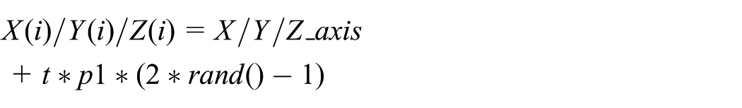
The distance of the fruit fly can then be obtained by

D (i) = (X (i)^2 + Y (i)^2 + Z (i)^2)^0.5

The smell concentration S(i) of the food is related to the distance function, which is utilized to guide the fruit fly to find the food

S (i) = abs (1 / D (i) + B_{1} - B_{2})

B is performed as an escaping factor to prevent the procedure from falling into the local minimum, which is initially set as 0 and calculate with the maximum and minimum location of each generation, the result of $B_{1} - B_{2}$ . It could act as a punishment factor to prevent overfitting and help the flies jump out from the local optimum area

Dis t_{\max} = \max (D (i)); Dis t_{\min} = \min (D (i))

B_{1 / 2} = 0.12 * Dis {t_{\max}}_{/ \min} * (0.5 - rand ())

Step 3: According to the fitness function and smell, the best individual could be obtained. The S(i) calculated before will be used as the input parameter of the fitness function which verifies the performance of each fruit fly, which is often set as the function of RMSE. In this case, the smaller the Smell(i) is, the better performance will be. Finally, the best location of this generation will be saved to judge whether the fruit fly should change the direction in the next run

Smell (i) = RMSE (S (i))

Step 4: According to the fitness function, update the best smell value. If the maximum generation is reached, the iteration will then end. If not, the procedure will turn to Step 5. At the same time, if the smell value is smaller than the expectation value(error), the procedure will be stopped to prevent the over-training problem.

Step 5: Update the best individual location and return to Step 2.

Model setting

Preprocessing of the sample data

Considering the computing time and over-training problem, regularization should be applied, which constrains the learning algorithm to reduce out-of-sample error, especially when noise is present.²⁶ In this article, to be brief, we regularize the training and testing data set to the range of [–1, 1]. The parameters for the IFOA are: the control parameter: 1.2 and the initial escaping factor $B_{1} - B_{2}$ is set to 0.

Selection of fitness function

The RMSE function is adopted as the fitness function, which is widely used in other research. Since the difference is first squared before averaged, it is sensitive to large errors and thus is appropriate to be chosen as the fitness function

RMSE = \sqrt{\frac{\sum_{i = 1}^{n} {(Y_{i} - {Y'}_{i})}^{2}}{n}}

(3)

where $Y_{i}$ is the measured value and $Y'_{i}$ is the predicted value.

Evaluation criteria

To verify the prediction ability of the prediction model comprehensively, in this article, more than one criterion was adopted, such as the RMSE, accuracy, and coefficient of determination; the formulas of each criterion are listed as follows:

Fitness parameter

Fitness = \min (Smell (i))

(4)

Accuracy

A c c u r a c y = 1 - \frac{1}{m} \sum_{i = 1}^{m} | \frac{y_{i} - {y^{'}}_{i}}{y_{i}} | \times 100 %

(5)

Coefficient of determination

R^{2} = \frac{m {(\sum_{i = 1}^{m} {y'}_{i} y_{i} - \sum_{i = 1}^{m} {y'}_{i} \sum_{i = 1}^{m} y_{i})}^{2}}{{(m \sum_{i = 1}^{m} {y'}_{i})}^{2} - {(\sum_{i = 1}^{m} {y'}_{i})}^{2} (m \sum_{i = 1}^{m} {(y_{i})}^{2} - {(\sum_{i = 1}^{m} y_{i})}^{2})}

(6)

Case study

In real cutting process, tool wear usually consists of three different phases: the break in-period phase, the steady-state wear phase, and the failure phase. In the failure phase, the wear shows an exponential curve with the increasing tool temperature resulting in rapid deterioration of the machined workpiece. Thus, different cutting conditions with time feature are capable to reflect the tool flank wear.

The turning process was conducted by CK6143/100 CNC machine on ZMn13 high manganese cast steel whose diameter is 90 mm, with a carbide alloy tool whose rake angle γ = 2°, relief angle α = 8°, cutting edge angle kr = 35°. The experimental setup is shown in Figure 3, in which the strain gauge sensor is used to measure the cutting force, thermal couple (assembled in the cutter) is used to measure the cutting temperature, and laser displacement sensor is used to measure the tool vibration. Considering the importance of the cutting conditions, three parameters of cutting conditions were involved to build the prediction model: the cutting speed, feed rate, and depth of cut. In order to verify the validation of the proposed model with the effect of types of measured features. Two cases are presented. Case 1 is designed for the tool wear prediction with less features while Case 2 is designed for the tool wear prediction with more measured features. The details of the experimental setup can refer to Yang et al.²⁷

Figure 3.

Experimental setup.

Case 1

Four features were abstracted to train the model: the cutting speed, feed rate, and depth of cut and cutting time, after finishing the experiment. Each of them has two different levels to present the diversity of cutting conditions as shown in Table 1. Since the profile of the cutting tool wear is usually uneven, the maximum tool flank wear VB_max was selected as the monitoring object of this experiment, which is directly measured by the microscope. Every time the cutting tool followed the same cutting path and after one run, a new tool will be installed to continue with the new cutting condition.

Table 1.

Cutting conditions for Case 1.

No.	D (mm)	V (m/min)	F (mm/r)	Cutting times (s)
1	1.5	21	0.05	18
2	1.5	43	0.05	6
3	1.5	21	0.7	27
4	1.5	43	0.7	3
5	0.5	21	0.05	30
6	0.5	43	0.05	30
7	0.5	21	0.7	21
8	0.5	43	0.7	12

The training data are scaled into [–1, 1]; the city block distance is adopted due to the better performance than Gaussian kernel in this simulation. Seventy-two sample data are used for training, while the other eight sample data with different cutting conditions are used for validating the prediction model. Then different evaluation criteria were used to verify the prediction accuracy. With limited amount of sample data and to prevent the over-training problem, the training process was conducted 10 times and the average performance was recorded to avoid the randomness. In each training time, eight samples with different cutting conditions were selected for validating.

The comparison between the predicted tool wear using IFOA-GRNN and measured tool wear is listed in Table 2. To visually reflect the comparison between the predicted and measured tool wear, comparison results for No. 1 and No. 2 are shown in Figure 4. It should be noted that the PSO and original FOA method are used to optimize the spread parameters for GRNN. The comparison results using IFOA-GRNN, FOA-GRNN, and PSO-GRNN are also listed in Table 2. It is clear that the GRNN method can be used to predict the tool wear with an acceptable accuracy. Furthermore, prediction accuracy δ using each method is calculated by $δ = 1 - | {VB}_{\max}^{Predicted} - {VB}_{\max}^{Measured} | / {VB}_{\max}^{Predicted}$ , and the calculated results are listed in Table 2. We can see that the prediction accuracy using IFOA-GRNN achieves the best performance compared to the other two methods. The average prediction accuracy using the proposed IFOA-GRNN method is 93.67% while the average prediction accuracy using the other two methods are 92.66% and 88.71%, respectively. However, it should be noted that the prediction accuracy for No. 4 and No. 6 is smaller than 90% even using IFOA-GRNN, which means the prediction results are not so stable with the small input information (only the machining information). In order to show the effectiveness of the proposed method, the prediction results using least squares support vector machine (LSSVM) method are also compared in Table 2. The prediction accuracy using LSSVM is 90.16%, which is larger than that using IFOA-GRNN. The fitness parameter optimization process of IFOA-GRNN is shown in Figure 5, which demonstrates that this algorithm has a great ability to search global optimum quickly, and the R² is 0.8583 showing that the predicted results have a high accuracy.

Table 2.

Comparison of predicted and measured tool wear for Case 1 (mm).

No.	1	2	3	4	5	6	7	8	Mean
Measured wear	0.4	0.25	0.6	0.25	0.61	0.75	0.42	0.35	–
VB_max of IFOA-GRNN	0.4302	0.2677	0.6213	0.2752	0.6107	0.6175	0.4212	0.335	–
VB_max of FOA-GRNN	0.4006	0.2897	0.5947	0.2808	0.6027	0.5915	0.4426	0.3572	–
VB_max of PSO-GRNN	0.4183	0.3112	0.5671	0.2839	0.5631	0.5288	0.4161	0.3349	–
VB_max of LSSVM	0.413	0.2246	0.6217	0.2543	0.4651	0.5682	0.4643	0.35	–
Accuracy of IFOA-GRNN	92.45	92.92	96.45	89.92	99.85	82.33	99.71	95.71	93.67
Accuracy of FOA-GRNN	99.85	84.42	99.12	87.68	98.8	78.87	94.62	97.94	92.66
Accuracy of PSO-GRNN	95.42	75.72	94.52	86.44	92.31	70.51	99.08	95.69	88.71
Accuracy of LSSVM	96.75	89.84	96.38	98.28	76.25	75.76	89.45	98.57	90.16

IFOA: improved fruit fly optimization algorithm; GRNN: general regression neural network; FOA: fruit fly optimization algorithm; PSO: particle swarm optimization; LSSVM: least squares support vector machine.

Figure 4.

Predicted and measured tool wear for each model in Case 1: (a) for No. 1 and (b) for No. 2.

Figure 5.

Optimization process of fitness parameter in Case 1.

Case 2

In the second case, more features obtained from multi-sensor were taken into consideration. The main cutting force, average cutting temperature, and the displacement of tool vibration were measured through diverse sensors during each run of the experiment. Cutting speed, feed rate, and depth of cut were designed with three different levels, as shown in Table 3.

Table 3.

Cutting conditions for Case 2.

No.	D (mm)	V (m/min)	F (mm/r)	Measured wear
1	0.3	60	0.05	0.1
2	0.3	70	0.07	0.17
3	0.3	70	0.05	0.155
4	0.5	70	0.05	0.185
5	0.3	50	0.05	0.07
6	0.3	50	0.06	0.08
7	0.3	50	0.07	0.09
8	0.4	50	0.05	0.08
9	0.4	50	0.06	0.08
10	0.4	50	0.07	0.105
11	0.5	50	0.05	0.085
12	0.5	50	0.06	0.095
13	0.5	50	0.07	0.11
14	0.3	60	0.06	0.12
15	0.3	60	0.07	0.155
16	0.4	60	0.05	0.105
17	0.4	60	0.06	0.135
18	0.4	60	0.07	0.17
19	0.5	60	0.05	0.12
20	0.5	60	0.06	0.14
21	0.5	60	0.07	0.18
22	0.3	70	0.06	0.155
23	0.4	70	0.05	0.18
24	0.4	70	0.06	0.16
25	0.4	70	0.07	0.175
26	0.5	70	0.06	0.185
27	0.5	70	0.07	0.19

Similar to the procedure in Case 1, the training process was conducted 10 times and the average performance was recorded. Each time four samples with different cutting conditions were randomly selected to validate the prediction model. The comparison between the predicted and measured tool wear is listed in Table 4. To visually reflect the comparison between the predicted and measured tool wear, comparison results for No. 1 and No. 2 are shown in Figure 6. It is clear that the GRNN method still can predict the tool wear. Similarly, IFOA-GRNN, FOA-GRNN, and PSO-GRNN method are compared and the comparison results are listed in Table 4. We can see that IFOA-GRNN still achieves the best performance compared to the other two methods. The average prediction accuracy is 96.37% while the accuracy for the other two methods are 92.74% and 91.06%, respectively. Compared to the accuracy in Case 1, the prediction accuracy is significantly improved. The reason is clear that more related information imported, better prediction accuracy achieved. The fitness parameter optimization process of IFOA-GRNN is shown in Figure 7 and the R² is 0.8799.

Table 4.

Comparison of predicted and measured tool wear (mm).

No.	Measured wear	VB_max of IFOA-GRNN	VB_max of FOA-GRNN	VB_max of PSO-GRNN	Accuracy of IFOA-GRNN	Accuracy of FOA-GRNN	Accuracy of PSO-GRNN
1	0.10	0.107	0.11	0.115	94.79	90	84.91
2	0.17	0.166	0.155	0.162	97.65	91.18	95.29
3	0.155	0.164	0.165	0.159	95.49	93.55	97.42
4	0.185	0.176	0.198	0.165	95.74	92.97	89.19
5	0.07	0.072	0.076	0.079	97.15	91.43	87.14
6	0.08	0.084	0.087	0.089	95	91.25	88.75
7	0.09	0.089	0.088	0.085	98.89	97.78	94.44
8	0.08	0.083	0.085	0.087	96.25	93.25	91.25
Mean					96.37	92.74	91.06

IFOA: improved fruit fly optimization algorithm; GRNN: general regression neural network; FOA: fruit fly optimization algorithm; PSO: particle swarm optimization.

Figure 6.

Predicted and measured tool wear for each model in Case 2: (a) for No. 1 and (b) for No. 2.

Figure 7.

Optimization process of fitness parameter in Case 2.

From these two case studies, some results can be concluded: (1) GRNN can be used to predict the tool wear with small or larger features under an acceptable accuracy; (2) more features added into the tool wear prediction model can improve the prediction accuracy; (3) IFOA method can automatically select the spread parameters for GRNN, which make the tool wear prediction model more automatically and accurate. In addition, the computation time for both cases using IFOA-GRNN is smaller than 1 s, which implies that the proposed method can be employed in the industry to monitor the tool wear condition with an acceptable computation time.

Conclusion

In this article, the generalized regression neural network (GRNN) is applied to solve the tool wear prediction/monitoring due to its excellent performance on learning speed and fast convergence to the optimal results regardless of whether the sample data are small or large. In order to avoid the low efficiency and accuracy caused by traditionally manual adjustment of the spread parameters in GRNN, the IFOA is proposed to optimize the spread parameters automatically considering different cutting conditions and relative parameters. Based on the proposed tool wear prediction method, the tool wear monitoring system can be established to guarantee that the cutting tool is always working under predefined tool wear criterion.

The proposed method is validated by various experiments and compared to the tool wear prediction method in the literature, that is, LSSVM. The comparison results show that the proposed method can predict the tool wear with a better performance.

As the spread parameters are automatically selected by IFOA, the computation time of the proposed method is below 1 s. In addition, the other optimization methods, PSO and FOA, are used to optimize the spread parameters in GRNN to verify the effectiveness of the proposed IFOA. From the comparison, IFOA-GRNN shows a better prediction ability than the PSO-GRNN and FOA-GRNN.

Although the proposed IFOA-GRNN can successfully predict the tool wear with small or large input information under an acceptable accuracy, we should acknowledge that the prediction accuracy may be quite large in some condition (17.67% in No. 6 of Case 1). However, this can be avoided with more input data including the measured force, temperature, and tool vibration signals using more sensors.

Footnotes

Handling Editor: Raffaella Sesana

Declaration of conflicting interests

The author(s) declared no potential conflicts of interest with respect to the research, authorship, and/or publication of this article.

Funding

The author(s) disclosed receipt of the following financial support for the research, authorship, and/or publication of this article: The study is supported by Chinese Universities Scientific Fund (grant no. 2018CDQYJX0013), National Natural Science Foundation (grant no. 51635003), and Innovation Team Development Program of the Ministry of Education (no. IRT_15R64).

ORCID iD

Ling Kang

References

Ghasempoor

Moore

Jeswiet

On-line wear estimation using neural networks. Proc IMechE, Part B: J Engineering Manufacture 1998; 212: 105–112.

Sick

On-line and indirect tool wear monitoring in turning with artificial neural networks: a review of more than a decade of research. Mech Syst Signal Pr 2002; 16: 487–546.

Fadare

Oni

AO.

Development and application of a machine vision system for measurement of surface roughness. J Eng Appl Sci 2009; 4.

Inoue

Konishi

Imai

Surface defect inspection of a cutting tool by image processing with neural networks. Mem Fac Eng—Okayama Univ 2009; 43: 55–60.

Cakan

Real-time monitoring of flank wear behavior of ceramic cutting tool in turning hardened steels. Int J Adv Manuf Technol 2011; 52: 897–903.

Barreiro

Castejón

Alegre

et al . Use of descriptors based on moments from digital images for tool wear monitoring. Int J Mach Tool Manuf 2008; 48: 1005–1013.

Xiong

Liu

Avila

Cutting tool wear measurement by using active contour model based image processing. In: Proceedings of the 2011 international conference on mechatronics and automation (ICMA), 2011, pp.670–675. IEEE.

Chelladurai

Jain

Vyas

NS.

Development of a cutting tool condition monitoring system for high speed turning operation by vibration and strain analysis. Int J Adv Manuf Technol 2008; 37: 471–485.

Chen

Huang

et al . Turning tool wear monitoring based on fuzzy cluster analysis. Lect Note Electr Eng 2010; 67: 739–745.

10.

Rangwala

Dornfeld

Sensor integration using neural networks for intelligent tool condition monitoring. J Eng Ind 1990; 112: 219–228.

11.

Dornfeld

Devries

MF.

Neural network sensor fusion for tool condition monitoring. CIRP Ann Manuf Technol 1990; 39: 101–105.

12.

Wen

Xiao

Yan

et al . Adjusting learning rate of memristor-based multilayer neural networks via fuzzy method. IEEE Trans Comput Aid Des Integ Circuit Syst 2018.

13.

Wen

Yang

et al . Memristor-based echo state network with online least mean square. IEEE Trans Syst Man Cyber Syst 2018; 1–10.

14.

Wen

Liu

Yang

et al . Generating realistic videos from keyframes with concatenated GANs. IEEE Trans Circuit Syst Video Technol 2018.

15.

Paul

Varadarajan

AS.

A multi-sensor fusion model based on artificial neural network to predict tool wear during hard turning. Proc IMechE, Part B: J Engineering Manufacture 2012; 226: 853–860.

16.

Shi

Gindy

NN.

Tool wear predictive model based on least squares support vector machines. Mech Syst Sig Proc 2007; 21: 1799–1814.

17.

Specht

DF.

A general regression neural network. IEEE Trans Neur Netw 1991; 2: 568–576.

18.

Aliustaoglu

Ertunc

Ocak

Tool wear condition monitoring using a sensor fusion model based on fuzzy inference system. Mech Syst Sig Proc 2009; 23: 539–546.

19.

Polat

Yıldırım

. Genetic optimization of GRNN for pattern recognition without feature extraction. Expert Syst Appl 2008; 34: 2444–2448.

20.

Xia

Lei

Wang

et al . GRNN short-term load forecasting model and virtual instrument design. Energy Procedia 2011; 13: 9150–9158.

21.

Ivic

Ibric

Betz . Optimization of drug release from compressed multi unit particle system (MUPS) using generalized regression neural network (GRNN). Arch Pharmacal Res 2010; 33: 103–113.

22.

Chen

Zhang

Long

et al . Research on surface roughness prediction model for high-speed milling inclined plane of hardened steel. Adv Mater Res 2010; 97–101: 2044–2048.

23.

Pan

WT.

A new fruit fly optimization algorithm: taking the financial distress model as an example. Knowl Based Syst 2012; 26: 69–74.

24.

Lin

. A novel 3D fruit fly optimization algorithm and its applications in economics. Neural Comput Appl 2015: 1–23.

25.

Wen

Zeng

et al . A short-term power load forecasting model based on the generalized regression neural network with decreasing step fruit fly optimization algorithm. Neurocomputing 2016; 221: 24–31.

26.

Xiao

Yang

Xing

et al . Clustering algorithm based on fruit fly optimization. Rough sets and knowledge technology. 2015, pp.408–419. Springer International Publishing.

27.

Yang

Wang

et al . A novel monitoring method for turning tool wear based on support vector machines. Proc Inst Mech Eng Part B J Eng Manuf 2016; 230.

Tool wear monitoring using generalized regression neural network

Abstract

Keywords

Introduction

IFOA-GRNN-based tool wear prediction model

Model setting

Preprocessing of the sample data

Selection of fitness function

Evaluation criteria

Case study

Case 1

Case 2

Conclusion

Footnotes

Declaration of conflicting interests

Funding

ORCID iD

References