Sage Journals: Discover world-class research

Abstract

The main objective of this article is to present a controller capable of maintaining a chain formation of platooning type, among a set of non-holonomic mobile robots, keeping a time-gap separation between each pair of consecutive robots at the platoon. It is intended that the whole set of robots asymptotically follows any feasible trajectory described by the leader robot. Under these conditions, the distance between any pair of consecutive robots, that is, the i-th robot and the (i + 1)-th robot, depends on the velocity of the i-th robot. Only position measurements are available, such that, to avoid using approximate velocity estimations, the chain formation problem is solved by considering a delay observer strategy. Based on the measurements of the positions of the robots, along the platoon, a delay observer is built for the i-th robot that provides a virtual reference for the (i + 1)-th robot, and this reference corresponds to the i-th robot trajectory delayed specific units of time, corresponding to the desired time-gap separation. Convergence of the (i + 1)-th robot to its desired delayed trajectory, which implies convergence of the chain formation, is formally proved by means of a Lyapunov stability approach and supported by numerical simulations and real-time experiments.

Keywords

Mobile robots observer based feedback intelligent robots time-gap separation

Introduction

The control problem of a set of mobile robots has been studied for several years, multiple related problems have been considered, for example, consensus, formation or synchronization of a set of robots, subject to specific constraints, which could be related to position or velocity relations among the robots. In particular, consensus, formation and synchronization problems have been considered in several works in the literature under a variety of formation conditions^1
–3; also in a more involved situation, the nonlinear case has been considered.⁴ The case when a set of robots, in a particular formation, has to follow the same path described by a leader robot is especially important when the robots must follow a predetermined trajectory inside a factory ambient or in archaeological exploring tasks where a leader robot goes through a tunnel or follows a specific path. This approach can be extended to vehicles, where traffic conditions can be seen as a platoon formation problem.

In the case of a pair of vehicles, the leader–follower formation has been studied using the relative distance between robots⁵; based on local motion sensors to perform the formation⁶ or by means of camera on board, the follower robot determines the relative distance between the vehicles.

Most of the solutions to the leader–follower formation problem consider a constant desired longitudinal distance and an angle between robots,^5,7

–11 for that reason, normally occurs that the follower robot hardly tracks the same path described by the leader robot, as in Cruz-Morales et al.,⁸ where a discrete time approach, camera on board, and a fixed distance between robots are used to perform the formation; here it is evident that when the leader robot tracks a curved path, the follower robot tends to describe a parallel path instead of the path described by the leader robot.

The leader–follower formation has also been extended for a set of follower robots, similar to the case of a pair of robots, where the formation is performed using a desired longitudinal distance and a desired angle between any pair of robots,^9,11

–15 where it is also considered using local sensors,^16,17 roof cameras,^18,19 or camera on board in the follower robots.²⁰ The use of GPS to obtain the position of the follower robots and performing the formation has also been studied.²¹

Following the same path executed by the leader vehicle could be of paramount importance, for instance, in the case of a chain formation of a set of vehicles in real traffic situations. The idea of vehicles following a predetermined road has been studied as a platoon formation, using a leader–follower string. Different controllers for a set of robots are given in previous studies,^10,22 where a formation is performed with a specific distance between robots that track the same path. In Klancar et al.,²³ two different approaches are shown: one uses a constant distance between mobile robots, and the other one uses a constant time separation approach to perform the platoon control.

The idea of having a time-gap separation between vehicles has been considered on the adaptive cruise control (ACC),^24

–27 where normally the platoon formation control starts when the vehicles are in linear formation after the initial tracking error have converged to zero by means of an additional control strategy; also, to maintain the formation, a bounded linear velocity is required. The main objectives of the ACC are described by Marsden et al.,²⁴ where a minimum time separation between vehicles is considered based on simulations and real-time driving conditions. In ACC, the goal is to control the translational velocity to enforce time and safe distance separation between vehicles and letting the steering task to the driver. Commonly, mass point and acceleration models are used at ACC to design the control strategy. The use of double integrator model for the vehicles together with a linear control strategy is presented by Swaroop and Rajagopal,²⁵ while Liu et al.²⁶ consider a linear velocity model including time-delay communication in the vehicle platoon. Also, a velocity model is considered by Bareket et al.,²⁷ where a discrete time approach is taken into account. The ACC strategy has shown that maintaining a time-gap separation is safer than keeping a fixed distance between vehicles.²³ Nevertheless, following a practical perspective, some limitations of the ACC are pointed out by Seppelt and Lee.²⁸

Looking for enhancing the performance of ACC, vehicle-to-vehicle communication (V2V) has been incorporated, yielding the so-called cooperative adaptive cruise control (CACC).²⁹ The exchange of information between vehicles renders the cooperative behavior, allowing smaller time and distance separation than ACC, while increasing safety. Nonetheless, there are some stability issues related to communication failure, delays at communication, information packet loss, and so on.³⁰ As mentioned in ACC and CACC, each vehicle at the platoon keeps a constant headway and safe distance with respect to its predecessor, which makes maneuvers such as merging or splitting of vehicles difficult. To help executing such maneuvers not only communication between vehicles has been considered, but also the behavior between the vehicles at the platoon and the rendering consensus at the formation.³¹

In the proposed approach, translational and rotational velocities are controlled at a differential mobile robot for not only keeping a time separation as in ACC and CACC but also simultaneously ensuring that the follower robot tracks the path of its predecessor at the platoon in position and orientation. For that, instead of considering a simplified or approximated model of the vehicles, in this article a solution for a platoon chain formation of a set of non-holonomic, differentially driven, mobile robots based on its kinematic model is proposed. It is intended that all the vehicles follow the same path described by the leader robot on the working space, considering a time gap between any pair of consecutive robots, instead of a constant distance. The formulation of the problem can be seen as a time-gap separation problem among vehicles in the formation. To solve the described problem, based on the measurement of the position of the i-th robot, a delayed observer that is able to provide the position and velocities of the i-th robot delayed τ units of time is proposed. This delayed estimated trajectory will serve as a desired reference for the (i + 1)-th robot in the platoon formation. In this way, the proposed strategy is able to maintain a given time-gap separation among the set of robots in the platoon. The leader robot, or first robot in the formation, is free to perform any feasible trajectory generated by arbitrary translational and rotational bounded inputs. The presented strategy is formally proven by a Lyapunov stability analysis.

In the rest of the article, first, the kinematic model of a set of mobile robots and the time-gap problem formulation are presented. Then, an input delay observer for the i-th robot is designed and the convergence of the observation errors is formally proven. Using this observer, the control law for the time-gap formation strategy for the (i + 1)-th robot is developed and, using a Lyapunov approach, the stability of the resulting closed-loop system is formally established. Simulations and real-time experiments are carried out to show the effectiveness of the proposed solution. Finally, some general conclusions are presented.

Kinematic model and problem formulation

A set of n differentially driven mobile robots of the type (2,0) is considered. The kinematic model of these robots can be easily obtained by considering the geometric relations depicted in Figure 1, producing the i-th robot model³²

\begin{array}{l} {\dot{x}}_{1 i} (t) = u_{1 i} (t) cos x_{3 i} (t) \\ {\dot{x}}_{2 i} (t) = u_{1 i} (t) sin x_{3 i} (t) \\ {\dot{x}}_{3 i} (t) = u_{2 i} (t) \end{array}

Figure 1.

Differentially driven mobile robot.

where the coordinates of the middle point of the wheel axis in the X–Y plane are denoted by (x _1i, x _2i), x _3i is the orientation angle of the vehicle with respect to X, and u _1i, u _2i are the translational and rotational input velocities, respectively. It is assumed that the mobile robots are made of rigid bodies, the wheels are non-deformable and they move on a horizontal plane, the contact between the wheels and the ground is on a single point of the plane and satisfy the pure rolling and non-slipping conditions along the motion. The robots fulfill the non-holonomic constraint

{\dot{x}}_{1 i} sin x_{3 i} - {\dot{x}}_{2 i} cos x_{3 i} = 0

for i = 1,2, ..., n.

Problem formulation

A platoon chain formation for a set of n differentially driven mobile robots is addressed in this work by considering the first robot as the leader of the formation. Instead of considering a fixed distance and orientation between each pair of consecutive robots in the formation, it is considered a fixed time-gap separation to be set between any pair of consecutive vehicles. The described platoon formation is depicted in Figure 2, where the robots are numbered i = 1,2, ..., n, starting at the leader robot (i = 1).

Figure 2.

Observer-based chain formation for n robots.

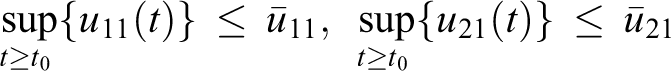
It is assumed that the leader robot (i = 1) performs any trajectory generated by bounded translational u ₁₁(t) and rotational u ₂₁(t) velocities. Under the assumption of bounded inputs and subject to restriction (2), the leader robot then describes a feasible trajectory on the X–Y plane. It is intended that the follower robots (i = 2, ..., n) track the path described by the leader robot with a time-gap of τ units of time between any pair of consecutive robots in the platoon formation. Under these conditions, τ represents a desired time-gap separation between the i-th robot and the (i + 1)-th robot, while performing the path established by the leader.

To solve the mentioned problem, along the platoon formation, the trajectory performed by the i-th robot, delayed τ units of time, will represent the desired trajectory for the (i + 1)-th robot. In this way, the i-th robot will take the delayed trajectory (τ units of time) of the (i + 1)-th robot as a desired trajectory and will generate the delayed desired trajectory for the (i + 1)-th robot.

Assuming that only the position of each robot is available for measurement, the desired position and velocity of the delayed trajectory for the (i + 1)-th robot will be obtained by means of an input-delayed observer based only on the current position of the i-th robot, that is, the (i + 1)-th robot will track the delayed position and velocity provided by the observer built for the i-th robot. The desired trajectories generated by the delayed observers, as well as the time-gap τ, are depicted in Figure 2, where the observer trajectories are denoted by the variables w _1i, w _2i, and w _3i.

Input delay observer design

To generate a feasible desired trajectory for the chain formation, it is assumed that the leader robot (robot 1) satisfies a bounded input assumption.

Assumption 1

The translational and rotational velocities of the leader mobile robot, i = 1, are bounded for all time t, that is,

$sup_{t \geq t_{0}} {u_{11} (t)} \leq {\bar{u}}_{11}, sup_{t \geq t_{0}} {u_{21} (t)} \leq {\bar{u}}_{21}$

for some positive constants ${\bar{u}}_{11}, {\bar{u}}_{21}$ and t ₀ = 0.

Considering the i-th robot, the development of an input delay observer to estimate the delayed (τ units of time) position and velocity trajectories of the i-th robot is carried out by considering the following additional assumption.

Assumption 2

The posture of the i-th mobile robot, x _1i(t), x _2i(t), x _3i(t) is available for measurement.

Consider the kinematic model of the i-th robot given by equation (1) and the following delayed variables

$\begin{array}{r} w_{1 i} (t) = x_{1 i} (t - τ) \\ w_{2 i} (t) = x_{2 i} (t - τ) \\ w_{3 i} (t) = x_{3 i} (t - τ) \end{array}$
3

The time derivative of (3) produces a virtual delayed representation of system (1) in the form

$\begin{array}{l} {\dot{w}}_{1 i} (t) = u_{1 i} (t - τ) cos w_{3 i} (t) \\ {\dot{w}}_{2 i} (t) = u_{1 i} (t - τ) sin w_{3 i} (t) \\ {\dot{w}}_{3 i} (t) = u_{2 i} (t - τ) \end{array}$
4

that allows to propose a delay observer for the virtual system (4) as

$\begin{array}{l} {\dot{\hat{w}}}_{1 i} (t) = u_{1 i} (t - τ) cos {\hat{w}}_{3 i} (t) + λ_{1 i} e_{w_{1 i}} (t) \\ {\dot{\hat{w}}}_{2 i} (t) = u_{1 i} (t - τ) sin {\hat{w}}_{3 i} (t) + λ_{2 i} e_{w_{2 i}} (t) \\ {\dot{\hat{w}}}_{3 i} (t) = u_{2 i} (t - τ) + λ_{3 i} e_{w_{3 i}} (t) \end{array}$
5

where

$\begin{array}{r} e_{w_{1 i}} (t) = w_{1 i} (t) - {\hat{w}}_{1 i} (t) = x_{1 i} (t - τ) - {\hat{w}}_{1 i} (t) \\ e_{w_{2 i}} (t) = w_{2 i} (t) - {\hat{w}}_{2 i} (t) = x_{2 i} (t - τ) - {\hat{w}}_{2 i} (t) \\ e_{w_{3 i}} (t) = w_{3 i} (t) - {\hat{w}}_{3 i} (t) = x_{3 i} (t - τ) - {\hat{w}}_{3 i} (t) \end{array}$
6

are the observation error variables, and λ _1i, λ _2i, λ _3i are positive constant design gains.

Remark 3

It is important to note that since the position of the i-th robot is available, the delayed position values can be obtained by simply storing them, and the delayed velocities might be estimated, for instance, by means of their approximation by a dirty derivative or by a discrete-time odometry-based estimation strategy. Notice that the use of approximate velocity estimation may prevent to formally prove the corresponding error convergence. This is the reason to use the delay observer (5), which not only gives the desired delayed position but also the estimated desired delayed velocities ${\dot{\hat{w}}}_{j i}$ for j = 1, 2, 3 of the i-th robot that will be used to design a tracking control law for the (i + 1)-th robot in the next section and in the analysis of the closed-loop system.

Observation error analysis

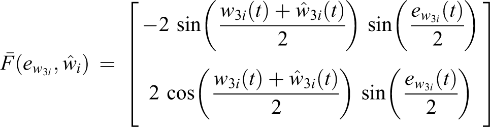
The observation error dynamics can be obtained by considering the time derivative of equation (6). The use of trigonometric identities allows to write

$\begin{array}{l} {\dot{e}}_{w_{1 i}} (t) = - λ_{1 i} e_{w_{1 i}} (t) \\ - 2 sin (\frac{e_{w_{3 i}} (t)}{2} + {\hat{w}}_{3 i} (t)) sin (\frac{e_{w_{3 i}} (t)}{2}) u_{1 i} (t - τ) \\ {\dot{e}}_{w_{2 i}} (t) = - λ_{2 i} e_{w_{2 i}} (t) \\ + 2 cos (\frac{e_{w_{3 i}} (t)}{2} + {\hat{w}}_{3 i} (t)) sin (\frac{e_{w_{3 i}} (t)}{2}) u_{1 i} (t - τ) \\ {\dot{e}}_{w_{3 i}} (t) = - λ_{3 i} e_{w_{3 i}} (t) \end{array}$
7

that can be rewritten as

${\dot{e}}_{w_{i}} (t) = A_{i} e_{w_{i}} (t) + F (e_{w_{3 i}}, {\hat{w}}_{i}) u_{1 i} (t - τ)$
8

where $e_{w_{i}} (t) = {[\begin{matrix} e_{w_{1 i}} (t) & e_{w_{2 i}} (t) & e_{w_{3 i}} (t) \end{matrix}]}^{T}$ and

$\begin{matrix} A_{i} = [\begin{matrix} - λ_{1 i} & 0 & 0 \\ 0 & - λ_{2 i} & 0 \\ 0 & 0 & - λ_{3 i} \end{matrix}] \\ F (e_{w_{3 i}}, {\hat{w}}_{i}) = [\begin{matrix} - 2 sin (\frac{w_{3 i} (t) + {\hat{w}}_{3 i} (t)}{2}) sin (\frac{e_{w_{3 i}} (t)}{2}) \\ 2 cos (\frac{w_{3 i} (t) + {\hat{w}}_{3 i} (t)}{2}) sin (\frac{e_{w_{3 i}} (t)}{2}) \\ 0 \end{matrix}] \end{matrix}$

The next lemma formally states the convergence properties of the observer (5).

Lemma 4

Consider the i-th robot with bounded inputs u _1i and u _2i, in the formation of Figure 2 and suppose that assumption 2 is satisfied and that λ _1i, λ _2i, λ _3i > 0. Then, the state defined by the observer (5), asymptotically converges to the i-th robot trajectory delayed τ units of time.

Proof

Notice first that for λ _3i > 0

${\dot{e}}_{w_{3 i}} (t) = - λ_{3 i} e_{w_{3 i}} (t)$

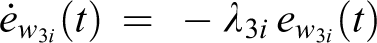
is exponentially stable. Therefore, the problem reduces to demonstrate that $e_{w_{1 i}} (t)$ and $e_{w_{2 i}} (t)$ also converge to the origin. With this aim, define

${\bar{e}}_{w_{i}} (t) = {[\begin{matrix} e_{w_{1 i}} (t) & e_{w_{2 i}} (t) \end{matrix}]}^{T}$

Then, the dynamics of ${\bar{e}}_{w_{i}} (t)$ can be expressed in the form

${\dot{\bar{e}}}_{w_{i}} (t) = {\bar{A}}_{i} {\bar{e}}_{w_{i}} (t) + \bar{F} (e_{w_{3 i}}, {\hat{w}}_{i}) u_{1 i} (t - τ)$
9

where

${\bar{A}}_{i} = [\begin{matrix} - λ_{1 i} & 0 \\ 0 & - λ_{2 i} \end{matrix}]$

and

$\bar{F} (e_{w_{3 i}}, {\hat{w}}_{i}) = [\begin{matrix} - 2 sin (\frac{w_{3 i} (t) + {\hat{w}}_{3 i} (t)}{2}) sin (\frac{e_{w_{3 i}} (t)}{2}) \\ 2 cos (\frac{w_{3 i} (t) + {\hat{w}}_{3 i} (t)}{2}) sin (\frac{e_{w_{3 i}} (t)}{2}) \end{matrix}]$

To show the convergence to the origin of ${\bar{e}}_{w_{i}} (t)$ , notice that

$\begin{matrix} | | \bar{F} (e_{w_{3 i}}, {\hat{w}}_{i}) u_{1 i} (t - τ) | | \leq | | \bar{F} (e_{w_{3 i}}, {\hat{w}}_{i}) | | | u_{1 i} (t - τ) | \\ \leq β_{i} | e_{w_{3 i}} | {\bar{u}}_{1 i} \end{matrix}$

for a suitable β_i > 0. Therefore, $\bar{F} (e_{w_{3 i}}, {\hat{w}}_{i})$ tends to zero as $e_{w_{3 i}} (t)$ converges to the origin, regardless of the evolution of $e_{w_{1 i}} (t)$ and $e_{w_{2 i}} (t)$ . Therefore, $\bar{F} (e_{w_{3 i}}, {\hat{w}}_{i}) u_{1 i} (t - τ)$ can be seen as a vanishing exogenous input signal for system (9), implying asymptotic convergence of the observation errors $e_{w_{1 i}} (t)$ , $e_{w_{2 i}} (t)$ since ${\bar{A}}_{i}$ is a Hurwitz matrix. This concludes the proof.

Remark 5

Notice that assumption 1 is a logical physical restriction for the leader robot (i = 1) that imposes a trajectory on the workspace that will be tracked, delayed τ units of time, by the second robot. In this way, along the platoon chain formation, the trajectory performed by the i-th robot, delayed τ units of time, will be considered the reference trajectory for the (i + 1)-th robot.

Remark 6

Notice that the input boundedness assumption in lemma 4 is relaxed for the controlled chain formation to only ask input boundedness of the leader robot as stated in assumption 1.

In what follows, for any pair of consecutive robots in the formation, the estimated state vector ${\hat{w}}_{i} (t) = {[{\hat{w}}_{1, i} {\hat{w}}_{2, i} {\hat{w}}_{3, i}]}^{T}$ will be used as a desired trajectory for the (i + 1)-th robot to solve in this way the considered time-gap platoon formation problem.

Observer-based time-gap platoon formation strategy

The control of the platoon chain formation described in Figure 2 can be synthesized by considering two consecutive mobile robots, lets say, i-th robot and (i + 1)-th robot. As mentioned earlier, the trajectory described by the i-th robot, delayed τ units of time, by the delay observer (5), will be considered as the desired trajectory for the (i + 1)-th robot. With this aim, consider the kinematic model of the (i + 1)-th robot

$\begin{array}{l} {\dot{x}}_{1 (i + 1)} (t) = u_{1 (i + 1)} (t) cos x_{3 (i + 1)} (t) \\ {\dot{x}}_{2 (i + 1)} (t) = u_{1 (i + 1)} (t) sin x_{3 (i + 1)} (t) \\ {\dot{x}}_{3 (i + 1)} (t) = u_{2 (i + 1)} (t) . \end{array}$
10

To solve the platoon formation problem, a feedback control law can be synthesized by means of a pair of virtual control inputs ξ _1(i+1)(t), ξ _2(i+1)(t) associated with system (10) in the form

$\begin{array}{r} {\dot{x}}_{1 (i + 1)} (t) = ξ_{1 (i + 1)} (t) \\ {\dot{x}}_{2 (i + 1)} (t) = ξ_{2 (i + 1)} (t) \\ {\dot{x}}_{3 (i + 1)} (t) = u_{2 (i + 1)} (t) . \end{array}$
11

Therefore, for system (10), it is possible to get

$u_{1 (i + 1)} (t) = ξ_{1 (i + 1)} (t) cos x_{3 (i + 1)} (t) + ξ_{2 (i + 1)} (t) sin x_{3 (i + 1)} (t)$
12

where the virtual inputs ξ _1(i+1)(t), ξ _2(i+1)(t) can be defined based on the observed desired reference as

$\begin{matrix} ξ_{1 (i + 1)} (t) = {\dot{\hat{w}}}_{1 i} (t) - k_{1 (i + 1)} (x_{1 (i + 1)} (t) - {\hat{w}}_{1 i} (t)) \\ ξ_{2 (i + 1)} (t) = {\dot{\hat{w}}}_{2 i} (t) - k_{2 (i + 1)} (x_{2 (i + 1)} (t) - {\hat{w}}_{2 i} (t)) \end{matrix}$
13

From the above developments, defining a set of tracking errors as

$\begin{array}{r} e_{s_{1 (i + 1)}} (t) = x_{1 (i + 1)} (t) - {\hat{w}}_{1 i} (t) \\ e_{s_{2 (i + 1)}} (t) = x_{2 (i + 1)} (t) - {\hat{w}}_{2 i} (t) \\ e_{s_{3 (i + 1)}} (t) = x_{3 (i + 1)} (t) - {\hat{w}}_{3 i} (t) \end{array}$
14

it is possible to propose the control signals in the form

$\begin{array}{l} u_{1 (i + 1)} (t) = ({\dot{\hat{w}}}_{1 i} (t) - k_{1 (i + 1)} e_{s_{1 (i + 1)}} (t)) cos x_{3 (i + 1)} (t) \\ + ({\dot{\hat{w}}}_{2 i} (t) - k_{2 (i + 1)} e_{s_{2 (i + 1)}} (t)) sin x_{3 (i + 1)} (t) \\ u_{2 (i + 1)} (t) = {\dot{\hat{w}}}_{3 i} (t) - k_{3 (i + 1)} e_{s_{3 (i + 1)}} (t) . \end{array}$
15

Remark 7

Notice that the definition of the virtual inputs ξ _1(i+1)(t) and ξ _2(i+1)(t) allows to synthesize the feedback control u _1(i+1)(t). Also, note that feedback (15) is free of singularities as it is a common issue in the case of feedback linearization–based solutions.³³

Tracking error convergence

Closed-loop systems (10) to (15) are described as

$\begin{matrix} {\dot{x}}_{1 (i + 1)} (t) = [({\dot{\hat{w}}}_{1 i} (t) - k_{1 (i + 1)} e_{s_{1 (i + 1)}} (t)) cos x_{3 (i + 1)} (t) + ({\dot{\hat{w}}}_{2 i} (t) - k_{2 (i + 1)} e_{s_{2 (i + 1)}} (t)) sin x_{3 (i + 1)} (t)] cos x_{3 (i + 1)} (t) \end{matrix}$
16

$\begin{matrix} {\dot{x}}_{2 (i + 1)} (t) = [({\dot{\hat{w}}}_{1 i} (t) - k_{1 (i + 1)} e_{s_{1 (i + 1)}} (t)) cos x_{3 (i + 1)} (t) + ({\dot{\hat{w}}}_{2 i} (t) - k_{2 (i + 1)} e_{s_{2 (i + 1)}} (t)) sin x_{3 (i + 1)} (t)] sin x_{3 (i + 1)} (t) \end{matrix}$
17

${\dot{x}}_{3 (i + 1)} (t) = {\dot{\hat{w}}}_{3 i} (t) - k_{3 (i + 1)} e_{s_{3 (i + 1)}} (t)$
18

From equation (18), it is possible to obtain

${\dot{e}}_{s_{3 (i + 1)}} (t) = - k_{3 (i + 1)} e_{s_{3 (i + 1)}} (t)$
19

Now, from (16)

${\dot{x}}_{1 (i + 1)} (t) = ({\dot{\hat{w}}}_{1 i} (t) - k_{1 (i + 1)} e_{s_{1 (i + 1)}} (t)) {cos}^{2} x_{3 (i + 1)} (t) + ({\dot{\hat{w}}}_{2 i} (t) - k_{2 (i + 1)} e_{s_{2 (i + 1)}} (t)) sin x_{3 (i + 1)} (t) cos x_{3 (i + 1)} (t) = ({\dot{\hat{w}}}_{1 i} (t) - k_{1 (i + 1)} e_{s_{1 (i + 1)}} (t)) (1 - {sin}^{2} x_{3 (i + 1)} (t)) + ({\dot{\hat{w}}}_{2 i} (t) - k_{2 (i + 1)} e_{s_{2 (i + 1)}} (t)) sin x_{3 (i + 1)} (t) cos x_{3 (i + 1)} (t)$

equivalently

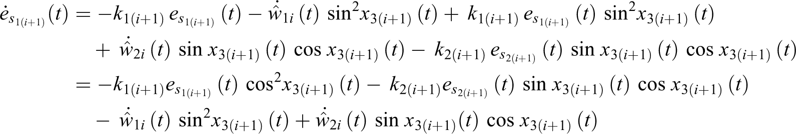
${\dot{e}}_{s_{1 (i + 1)}} (t) = - k_{1 (i + 1)} e_{s_{1 (i + 1)}} (t) - {\dot{\hat{w}}}_{1 i} (t) {sin}^{2} x_{3 (i + 1)} (t) + k_{1 (i + 1)} e_{s_{1 (i + 1)}} (t) {sin}^{2} x_{3 (i + 1)} (t) + {\dot{\hat{w}}}_{2 i} (t) sin x_{3 (i + 1)} (t) cos x_{3 (i + 1)} (t) - k_{2 (i + 1)} e_{s_{2 (i + 1)}} (t) sin x_{3 (i + 1)} (t) cos x_{3 (i + 1)} (t) = - k_{1 (i + 1)} e_{s_{1 (i + 1)}} (t) {cos}^{2} x_{3 (i + 1)} (t) - k_{2 (i + 1)} e_{s_{2 (i + 1)}} (t) sin x_{3 (i + 1)} (t) cos x_{3 (i + 1)} (t) - {\dot{\hat{w}}}_{1 i} (t) {sin}^{2} x_{3 (i + 1)} (t) + {\dot{\hat{w}}}_{2 i} (t) sin x_{3 (i + 1)} (t) cos x_{3 (i + 1)} (t)$

Substituting ${\dot{\hat{w}}}_{1 i} (t)$ and ${\dot{\hat{w}}}_{2 i} (t)$ from the observer dynamics (5), the following equation is obtained

${\dot{e}}_{s_{1 (i + 1)}} (t) = - k_{1 (i + 1)} e_{s_{1 (i + 1)}} (t) {cos}^{2} x_{3 (i + 1)} (t) - k_{2 (i + 1)} e_{s_{2 (i + 1)}} (t) sin x_{3 (i + 1)} (t) cos x_{3 (i + 1)} (t) - λ_{1 i} e_{w_{1 i}} (t) {sin}^{2} x_{3 (i + 1)} (t) - u_{1 i} (t - τ) sin x_{3 (i + 1)} (t) sin e_{s_{3 (i + 1)}} (t) + λ_{2 i} e_{w_{2 i}} (t) sin x_{3 (i + 1)} (t) cos x_{3 (i + 1)} (t)$

Using a similar procedure for equation (17)

$\begin{matrix} {\dot{e}}_{s_{2 (i + 1)}} (t) = - k_{2 (i + 1)} e_{s_{2 (i + 1)}} (t) {sin}^{2} x_{3 (i + 1)} (t) - k_{1 (i + 1)} e_{s_{1 (i + 1)}} (t) cos x_{3 (i + 1)} (t) sin x_{3 (i + 1)} (t) \\ - {\dot{\hat{w}}}_{2 i} (t) {cos}^{2} x_{3 (i + 1)} (t) + {\dot{\hat{w}}}_{1 i} (t) cos x_{3 (i + 1)} (t) sin x_{3 (i + 1)} (t) \end{matrix}$
20

Then, the tracking error dynamics can be rewritten as

${\dot{e}}_{s_{1 (i + 1)}} (t) = - k_{1 (i + 1)} e_{s_{1 (i + 1)}} (t) {cos}^{2} (e_{s_{3 (i + 1)}} (t) + {\hat{w}}_{3 i} (t)) - k_{2 (i + 1)} e_{s_{2 (i + 1)}} (t) sin (e_{s_{3 (i + 1)}} (t) + {\hat{w}}_{3 i} (t)) \times cos (e_{s_{3 (i + 1)}} (t) + {\hat{w}}_{3 i} (t)) + m_{1 (i + 1)} (t) {\dot{e}}_{s_{2 (i + 1)}} (t) = - k_{1 (i + 1)} e_{s_{1 (i + 1)}} (t) cos (e_{s_{3 (i + 1)}} (t) + {\hat{w}}_{3 i} (t)) \times sin (e_{s_{3 (i + 1)}} (t) + {\hat{w}}_{3 i} (t)) - k_{2 (i + 1)} e_{s_{2 (i + 1)}} (t) {sin}^{2} (e_{s_{3 (i + 1)}} (t) + {\hat{w}}_{3 i} (t)) + m_{2 (i + 1)} (t) {\dot{e}}_{s_{3 (i + 1)}} (t) = - k_{3 (i + 1)} e_{s_{3 (i + 1)}} (t)$
21

where

$m_{1 (i + 1)} (t) = - u_{1 i} (t - τ) sin (e_{s_{3 (i + 1)}} (t) + {\hat{w}}_{3 i} (t)) sin e_{s_{3 (i + 1)}} (t) - λ_{1 i} e_{w_{1 i}} (t) {sin}^{2} (e_{s_{3 (i + 1)}} (t) + {\hat{w}}_{3 i} (t)) + λ_{2 i} e_{w_{2 i}} (t) sin (e_{s_{3 (i + 1)}} (t) + {\hat{w}}_{3 i} (t)) \times cos (e_{s_{3 (i + 1)}} (t) + {\hat{w}}_{3 i} (t)) m_{2 (i + 1)} (t) = u_{1 i} (t - τ) cos (e_{s_{3 (i + 1)}} (t) + {\hat{w}}_{3 i} (t)) sin e_{s_{3 (i + 1)}} (t) + λ_{2 i} e_{w_{2 i}} (t) {cos}^{2} (e_{s_{3 (i + 1)}} (t) + {\hat{w}}_{3 i} (t)) + λ_{1 i} e_{w_{1 i}} (t) cos (e_{s_{3 (i + 1)}} (t) + {\hat{w}}_{3 i} (t)) \times sin (e_{s_{3 (i + 1)}} (t) + {\hat{w}}_{3 i} (t))$

The above developments can now be formally stated as follows.

Lemma 8

Suppose that assumptions 1 and 2 are satisfied, that k _i+1 = k _1(i+1) = k _2(i+1) > 0, k _3(i+1) > 0 and that the desired angular velocity of the (i + 1)-th robot satisfies ${\dot{\hat{w}}}_{3 i} (t) \neq 0$ for all t. Then, the closed-loop tracking error dynamics given by (21) is asymptotically stable. Consequently, the observer-based feedback control (15) asymptotically solves the time-gap separation tracking problem associated with the considered platoon chain formation.

Proof

Note that the signals m _1(i+1)(t) and m _2(i+1)(t) depend on the observation errors $e_{w_{1 i}} (t), e_{w_{2 i}} (t)$ and on the tracking error $e_{s_{3 (i + 1)}} (t)$ . The asymptotic convergence of the observation errors has previously been proven, while the exponential convergence of $e_{s_{3 (i + 1)}} (t)$ can be easily established from (19). Therefore, m _1(i+1)(t), m _2(i+1)(t) → 0 as t → ∞ and they can be considered as vanishing exogenous input signals for the dynamics of $e_{s_{1 (i + 1)}} (t)$ and $e_{s_{2 (i + 1)}} (t)$ . As a consequence, the stability of system (21) can be stated by considering the non-perturbed system

${\dot{e}}_{s_{1 (i + 1)}} (t) = - k_{1 (i + 1)} e_{s_{1 (i + 1)}} (t) {cos}^{2} (e_{s_{3 (i + 1)}} (t) + {\hat{w}}_{3 i} (t)) - k_{2 (i + 1)} e_{s_{2 (i + 1)}} (t) sin (e_{s_{3 (i + 1)}} (t) + {\hat{w}}_{3 i} (t)) \times cos (e_{s_{3 (i + 1)}} (t) + {\hat{w}}_{3 i} (t)) {\dot{e}}_{s_{2 (i + 1)}} (t) = - k_{2 (i + 1)} e_{s_{2 (i + 1)}} (t) {sin}^{2} (e_{s_{3 (i + 1)}} (t) + {\hat{w}}_{3 i} (t)) - k_{1 (i + 1)} e_{s_{1 (i + 1)}} (t) cos (e_{s_{3 (i + 1)}} (t) + {\hat{w}}_{3 i} (t)) \times sin (e_{s_{3 (i + 1)}} (t) + {\hat{w}}_{3 i} (t))$
22

With this aim, consider now the candidate Lyapunov function

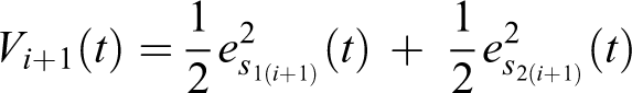
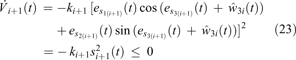
$V_{i + 1} (t) = \frac{1}{2} e_{s_{1 (i + 1)}}^{2} (t) + \frac{1}{2} e_{s_{2 (i + 1)}}^{2} (t)$

The time derivative of this function results in

${\dot{V}}_{i + 1} (t) = - k_{1 (i + 1)} e_{s_{1 (i + 1)}}^{2} (t) {cos}^{2} (e_{s_{3 (i + 1)}} (t) + {\hat{w}}_{3 i} (t)) - k_{1 (i + 1)} e_{s_{1 (i + 1)}} (t) e_{s_{2 (i + 1)}} (t) sin (e_{s_{3 (i + 1)}} (t) + {\hat{w}}_{3 i} (t)) \times cos (e_{s_{3 (i + 1)}} (t) + {\hat{w}}_{3 i} (t)) - k_{2 (i + 1)} e_{s_{1 (i + 1)}} (t) e_{s_{2 (i + 1)}} (t) sin (e_{s_{3 (i + 1)}} (t) + {\hat{w}}_{3 i} (t)) \times cos (e_{s_{3 (i + 1)}} (t) + {\hat{w}}_{3 i} (t)) - k_{2 (i + 1)} e_{s_{2 (i + 1)}}^{2} (t) {sin}^{2} (e_{s_{3 (i + 1)}} (t) + {\hat{w}}_{3 i} (t))$

From the hypothesis of the lemma, k _i+1 = k _1(i+1) = k _2(i+1), and defining $s_{i + 1} (t) = e_{s_{1 (i + 1)}} (t) cos (e_{s_{3 (i + 1)}} (t) + {\hat{w}}_{3 i} (t)) + e_{s_{2 (i + 1)}} (t) sin (e_{s_{3 (i + 1)}} (t) + {\hat{w}}_{3 i} (t))$

$\begin{matrix} {\dot{V}}_{i + 1} (t) = - k_{i + 1} [e_{s_{1 (i + 1)}} (t) cos (e_{s_{3 (i + 1)}} (t) + {\hat{w}}_{3 i} (t)) \\ + e_{s_{2 (i + 1)}} (t) sin (e_{s_{3 (i + 1)}} (t) + {\hat{w}}_{3 i} (t {))]}^{2} \\ = - k_{i + 1} s_{i + 1}^{2} (t) \leq 0 \end{matrix}$
23

that allows to assure the stability of system (22).

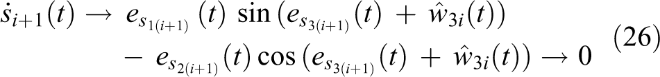
To show the asymptotic converge to the origin of (22), notice that ${\dot{V}}_{i + 1} (t)$ is differentiable and uniformly continuous since ${\ddot{V}}_{i + 1} (t)$ is bounded. By invoking Barbalat’s lemma,³⁴ ${\dot{V}}_{i + 1} (t) \to 0$ as t → ∞ and consequently, from (23)

$e_{s_{1 (i + 1)}} (t) cos (e_{s_{3 (i + 1)}} (t) + {\hat{w}}_{3 i} (t)) \to - e_{s_{2 (i + 1)}} (t) sin (e_{s_{3 (i + 1)}} (t) + {\hat{w}}_{3 i} (t))$
24

as t → ∞.

It is clear from the dynamics of system (22) that

${\dot{e}}_{s_{1 (i + 1)}} (t), {\dot{e}}_{s_{2 (i + 1)}} (t) \to 0 as t \to \infty$
25

Since ${\dot{V}}_{i + 1} (t) \to 0$ , the function s _i+1(t) also tends to the origin and consequently ${\dot{s}}_{i + 1} (t)$ also tends to zero.

Therefore, by considering (25) and since ${\dot{e}}_{s_{3 (i + 1)}} (t) \to 0$ , it is possible to see that ${\dot{s}}_{i + 1} (t) \to 0$ , as t → ∞, so

${\dot{s}}_{i + 1} (t) \to [e_{s_{1 (i + 1)}} sin (e_{s_{3 (i + 1)}} + {\hat{w}}_{3 i}) - e_{s_{2 (i + 1)}} cos (e_{s_{3 (i + 1)}} + {\hat{w}}_{3 i})] {\dot{\hat{w}}}_{3 i} \to 0$

Note that the above expression can be trivially satisfied by ${\dot{\hat{w}}}_{3 i} = 0$ , such that convergence of $(e_{s_{1 i}}, e_{s_{2 i}})$ cannot be drawn because it would depend on the values of $(e_{s_{1 i}}, e_{s_{2 i}})$ . But, from the hypothesis of the lemma, ${\dot{\hat{w}}}_{3 i} \neq 0$ , which implies that

$\begin{array}{l} {\dot{s}}_{i + 1} (t) \to e_{s_{1 (i + 1)}} (t) sin (e_{s_{3 (i + 1)}} (t) + {\hat{w}}_{3 i} (t)) \\ - e_{s_{2 (i + 1)}} (t) cos (e_{s_{3 (i + 1)}} (t) + {\hat{w}}_{3 i} (t)) \to 0 \end{array}$
26

From the fact that ${\dot{V}}_{i + 1} (t) \to 0$ , and considering (26), it can be obtained that

$[\begin{matrix} cos (e_{s_{3 (i + 1)}} (t) + {\hat{w}}_{3 i} (t)) & sin (e_{s_{3 (i + 1)}} (t) + {\hat{w}}_{3 i} (t)) \\ sin (e_{s_{3 (i + 1)}} (t) + {\hat{w}}_{3 i} (t)) & - cos (e_{s_{3 (i + 1)}} (t) + {\hat{w}}_{3 i} (t)) \end{matrix}] [\begin{matrix} e_{s_{1 (i + 1)}} \\ e_{s_{2 (i + 1)}} \end{matrix}] \to 0$

From the non-singularity of the involved matrix, $(e_{s_{1 (i + 1)}} (t), e_{s_{2 (i + 1)}} (t)) \to 0$ as t → ∞.

This concludes the proof.

Notice that from the above proof, stability of all the tracking errors at the platoon formation can be stated without any particular assumption. Nonetheless, in order to prove asymptotic convergence of $(e_{s_{1 i}}, e_{s_{2 i}})$ , the condition ${\dot{\hat{w}}}_{3 i} \neq 0$ is required. This condition seems to be rather conservative and less practical, but what it states is only a general convergence condition, thus, straight line paths are not let out of our framework. In fact, if the robots are to perform a straight line and they start in a position and orientation that the initial tracking errors $(e_{s_{1 i}}, e_{s_{2 i}}, e_{s_{3 i}})$ are zero, then they would remain zero, without the need of ${\dot{\hat{w}}}_{3 i} \neq 0$ .

On the other hand, if the initial conditions at the tracking errors $(e_{s_{1 i}}, e_{s_{2 i}}, e_{s_{3 i}})$ are different from zero, they will converge to zero, because $e_{s_{3 i}}$ is exponentially stable, and would imply that at the transient state till steady state is achieved, ${\dot{\hat{w}}}_{3 i} \neq 0$ .

The condition ${\dot{\hat{w}}}_{3 i} \neq 0$ is formerly required when the tracking errors $(e_{s_{1 i}}, e_{s_{2 i}})$ are non-zero, but simultaneously $e_{s_{3 i}} = 0$ , which implies parallel trajectories of the robots when performing a straight line path, in such case $(e_{s_{1 i}}, e_{s_{2 i}})$ , would remain stable and bounded, and will converge to zero when ${\dot{\hat{w}}}_{3 i} \neq 0$ is satisfied.

Remark 9

It should be pointed out that even when our work is inspired on the ACC, since a time-gap separation between any pair of consecutive robots is considered, contrary to the approximated model of the vehicles considered in the literatures,^24

–27 in this work, the kinematic model of the vehicles that include non-holonomic constraints is considered. Furthermore, not only translational velocity of the mobile robot is considered, but also rotational velocity, such that tracking of the path of the leader robot in position and orientation is ensured, while a constant headway is kept along the platoon.

Platoon chain formation strategy evaluation

The effectiveness of the observer-based formation strategy proposed in this work will be evaluated by means of numerical simulations and real-time experiments. Three differentially driven mobile robots that should track a geometric trajectory involving orientation and velocity changes for the leader robot (i = 1) will be considered, with the goal to show that the relative distance between the robots varies according to the velocity of the i-th robot.

The linear and angular velocities considered for robot 1 will be generated according to

$u_{11} = {\dot{\bar{x}}}_{11} cos {\bar{x}}_{31} + {\dot{\bar{x}}}_{21} sin {\bar{x}}_{31}, u_{21} = \frac{({\ddot{\bar{x}}}_{21} {\dot{\bar{x}}}_{11} - {\ddot{\bar{x}}}_{11} {\dot{\bar{x}}}_{21})}{({\dot{\bar{x}}}_{11}^{2} + {\dot{\bar{x}}}_{21}^{2})}$
27

for

$\begin{array}{l} {\bar{x}}_{11} = A cos (w t) \\ {\bar{x}}_{21} = B sin (2 w t) \\ {\bar{x}}_{31} = atan 2 (\frac{{\dot{\bar{x}}}_{21}}{{\dot{\bar{x}}}_{11}}) \end{array}$
28

where A = 1.5, B = 0.8, w = 0.15 and t ₀ ≤ t ≤ t_f , with t ₀ = 0 and t_f = 78s. Input signals (27) impose a Lemniscata shape trajectory for robot 1 and they are bounded as required. Note that in the experiment, a data pile is used, in which the position and orientation data of each robot are saved; this is done at each sampling period until τ units of time have passed, then the data are taken out from the pile; with this strategy, the variables x _1i(t − τ), x _2i(t − τ), x _3i(t − τ) are obtained, which are used in the delay observer (5).

Since the solution is based on an estimated state, from the structure of observer (5), it is clear that the inputs u _1i(t − τ) and u _2i(t − τ) start to affect the dynamics of the observer at time t ₀ + τ, producing a large transient signal for the feedback law injected to the robots. To alleviate this phenomenon, although the control signals are computed from t ₀, they are injected to the robot for t > t ₀ + τ, allowing a time lapse for the observer, to converge to the real values. This strategy is implemented in the numerical and real-time experiments to make a fair comparison.

Numerical evaluation

The numerical simulation is carried out by considering a time-gap separation of τ = 3.5 s. Since robot 1 is driven by inputs (27), it is required to control the remaining two robots. The gains considered for observer (5) are chosen as λ ₁₁ = λ ₂₁ = λ ₃₁ = 5, λ ₁₂ = λ ₂₂ = λ ₃₂ = 2, and the gains used for control law (15) are set as k _1i = 1, k _2i = 1, k _3i = 2 for i = 2, 3. The initial conditions for the simulation are shown in Table 1.

Table 1.
Initial conditions.

Robot x _1i(m) x _2i(m) x _3i(rad)

Robot 1 1.55 −0.035 1.612

Observer 1 1.55 −0.035 1.612

Robot 2 1.76 −0.072 1.59

Observer 2 1.76 −0.072 1.59

Robot 3 1.98 −0.082 1.468

The time evolution on the plane of the robots formation is shown in Figure 3.

Figure 3.
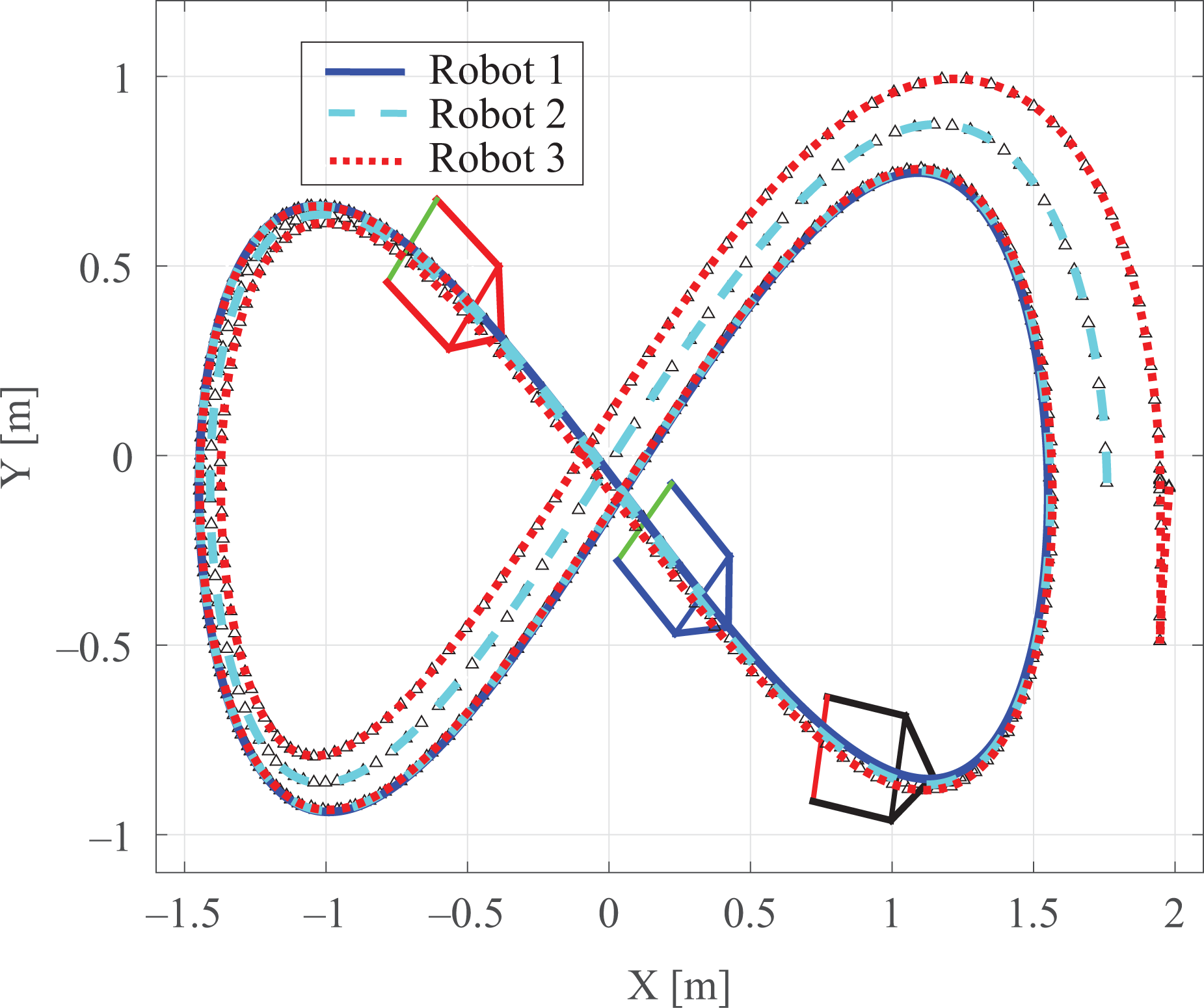
Time evolution of the platooning on the X–Y plane.

The observation errors $e_{w_{1 i}} (t)$ , $e_{w_{2 i}} (t)$ , $e_{w_{3 i}} (t)$ for i = 1, 2 are depicted in Figure 4 where their fast convergence to the origin as stated by lemma 4 is evident.

Figure 4.
Observation errors $e_{w_{1 i}} (t)$ , $e_{w_{2 i}} (t)$ , and $e_{w_{3 i}} (t)$ evolution.

The tracking position errors $e_{s_{1 i}} (t)$ , $e_{s_{2 i}} (t)$ , $e_{s_{3 i}} (t)$ for i = 2, 3 are shown in Figure 5. Notice that despite the initial condition errors, all the signals converge adequately as expected by the theoretical developments. The corresponding evolution of the control signals u _1i(t) and u _2i(t) for i = 1, 2, 3 is shown in Figure 6.

Figure 5.
Position tracking errors $e_{s_{1 i}} (t)$ , $e_{s_{2 i}} (t)$ , and $e_{s_{3 i}} (t)$ .

Figure 6.
Control signal evolution u _1i(t) and u _2i(t).

Finally, Figure 7 shows the evolution of the relative distances between the robots, $d_{i} (t) = \sqrt{{(x_{1 i} (t) - x_{1 (i + 1)} (t))}^{2} + {(x_{2 i} (t) - x_{2 (i + 1)} (t))}^{2})}$ , that varies according to the robots velocities in order to satisfy the time-gap separation.

Figure 7.
Relative distances d_i (t) between the robots.

Real-time experiments

The proposed controller is experimentally tested while performing the same Lemniscata shape trajectory (27) used in the numerical simulation study. Two cases are considered: the first one corresponds to the same conditions as in the simulation case and allows comparing predicted simulated results against experimental ones. The second case considers additive disturbances at the position and orientation of the second robot at the platoon, showing robustness properties of the proposed controller against disturbances. First, the experimental platform is described and then the experimental results are shown.

Experimental platform

To test the proposed platoon chain formation control law, an experimental platform is used to perform the same trajectory as for the numerical simulation. This experimental platform consists of three “Garcia” mobile robots of Acroname Inc, an indoor localization system, and a personal computer. The “Garcia” robots have two Maxon motors with encoder that generates 3648 ppr and use a 40 MHz processor and wireless communication. The localization system is equipped with 12 Flex-13 “Optitrack” cameras from Natural Point Inc., with an image resolution of 1280 × 1024 and a frame rate of 120 frame per second (FPS), covering an area of 20 m². The position information of the robots is obtained by means of the software “Motive” of the same company. A personal computer is used to calculate the control laws and to generate the control signals, and 12 cameras are connected to the computer where the Motive software is installed and the control laws are processed. The control signals are sent to the robots by wireless communication, and the experimental platform components are shown in Figure 8.

Figure 8.
Experimental platform diagram.

Since the mobile robots are actually driven by wheel velocities, the globally invertible relation is considered

$\begin{matrix} w_{l i} = \frac{1}{r} (u_{1 i} - u_{2 i} l) \\ w_{r i} = \frac{1}{r} (u_{1 i} + u_{2 i} l) \end{matrix}$
29

where r = 0.0508 m is the wheel radius and l = 0.1983 m is the length of the wheel axle; these equations allow to compute the i-th robot left w _li and right w _ri wheel velocities i = 1, 2, 3. The initial conditions for the experiment are also shown in Table 1.

The gains used at both experimental scenarios, with and without disturbances, are the same. For observer (5), the gains are λ ₁₁ = λ ₂₁ = λ ₃₁ = 2.5, λ ₁₂ = λ ₂₂ = λ ₃₂ = 3.0 and the gains used for control law (15) are set as k ₁₂ = k ₂₂ = k ₃₂ = 1.4 and k ₁₃ = k ₂₃ = k ₃₃ = 1.5. The time gap was also considered as τ = 3.5 s as in simulations.

Experimental results without disturbances

This case allows direct comparison with simulation results previously presented. Figure 9 shows some snapshots of the experiment, and Figure 10 shows the time evolution of the formation in the plane.

Figure 9.
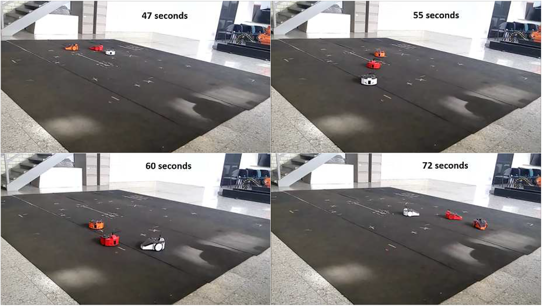
Real-time experiment without disturbances.

Figure 10.
Real-time experiment evolution of the platoon on the X–Y plane, without disturbances.

The observation errors $e_{w_{1 i}} (t), e_{w_{2 i}} (t), e_{w_{3 i}} (t)$ are depicted in Figure 11, where their fast convergence is shown, and both observers behave as expected. The tracking position errors $e_{s_{1 i}} (t), e_{s_{2 i}} (t)$ , and $e_{s_{3 i}} (t)$ are shown in Figure 12. Notice that these errors converge to zero as stated by the stability proof.

Figure 11.
Real-time experiment, observation errors without disturbances.

Figure 12.
Position tracking errors without disturbances.

In Figure 13, the control signals of the robots are shown. After 15 s, the behavior of the signals is as expected by the theoretical and simulations results, and the signals show the time-gap separation of τ units of time between them.

Figure 13.
Control signals evolution without disturbances.

Finally, Figure 14 shows how the separation or relative distance between the robots, d_i (t), behaves. It is important to notice that the numerical and real-time experiments have very similar behaviors between them, despite the well-known differences between a simulation and the real-time experiment, such as model errors, friction forces, slipping phenomena, mechanical issues of the robots, which are not considered on the kinematic model.

Figure 14.
Relative distance between robots, without disturbances.

Experimental results with disturbances

This case scenario considers that the position and orientation of the second mobile robot at the platoon are suddenly modified, as emulating an additive perturbation, which could be seen as a failure on the localization system. To favor a fair comparison with previous simulated and experimental results, the observer and controller gains are the same as for the experimental case without disturbances, and the desired path is the same Lemniscata trajectory. To test the performance and robustness of the proposed control law under disturbances effects, the second robot is twice manually taken out its path, affecting its position and mainly its orientation, and these perturbations occur at the 16th and 56th seconds of the experiment. Since the position and orientation of the robots are measured by the absolute localization system, then this abrupt change on position and orientation is feedback to the observer and the control law.

The initial conditions for the experiment are shown in Table 2.

Table 2.
Initial conditions: Real-time experiment with disturbances.

Robot x _1i(m) x _2i(m) x _3i(rad)

Robot 1 1.61 −0.19 1.51

Observer 1 1.61 −0.19 1.51

Robot 2 1.23 −0.75 1.32

Observer 2 1.23 −0.75 1.32

Robot 3 1.68 −0.74 1.71

The effects of disturbances at the 16th and 56th seconds are appreciated in Figures 15 and 16, where the position of each robot and observer are shown with respect to time. In each figure, it is possible to see the disturbance effects, but mainly at the orientation of the robot, where changes on orientation of approximately 0.5 and 1.0 (rad) are appreciated. It is seen that the position and orientation of the second robot are highly affected by the disturbance, but it is interesting how these effects are absorbed by the second observer, which is in charge of generating the desired trajectory for the third robot at the platoon, such that the third robot is closer to the leader trajectory than to the disturbed path of the second robot. This behavior is due to the filtering effect of the observer and that at the end, the leader trajectory is intrinsically propagated along the platoon chain formation by the observers and the controllers at each follower robot.

Figure 15.
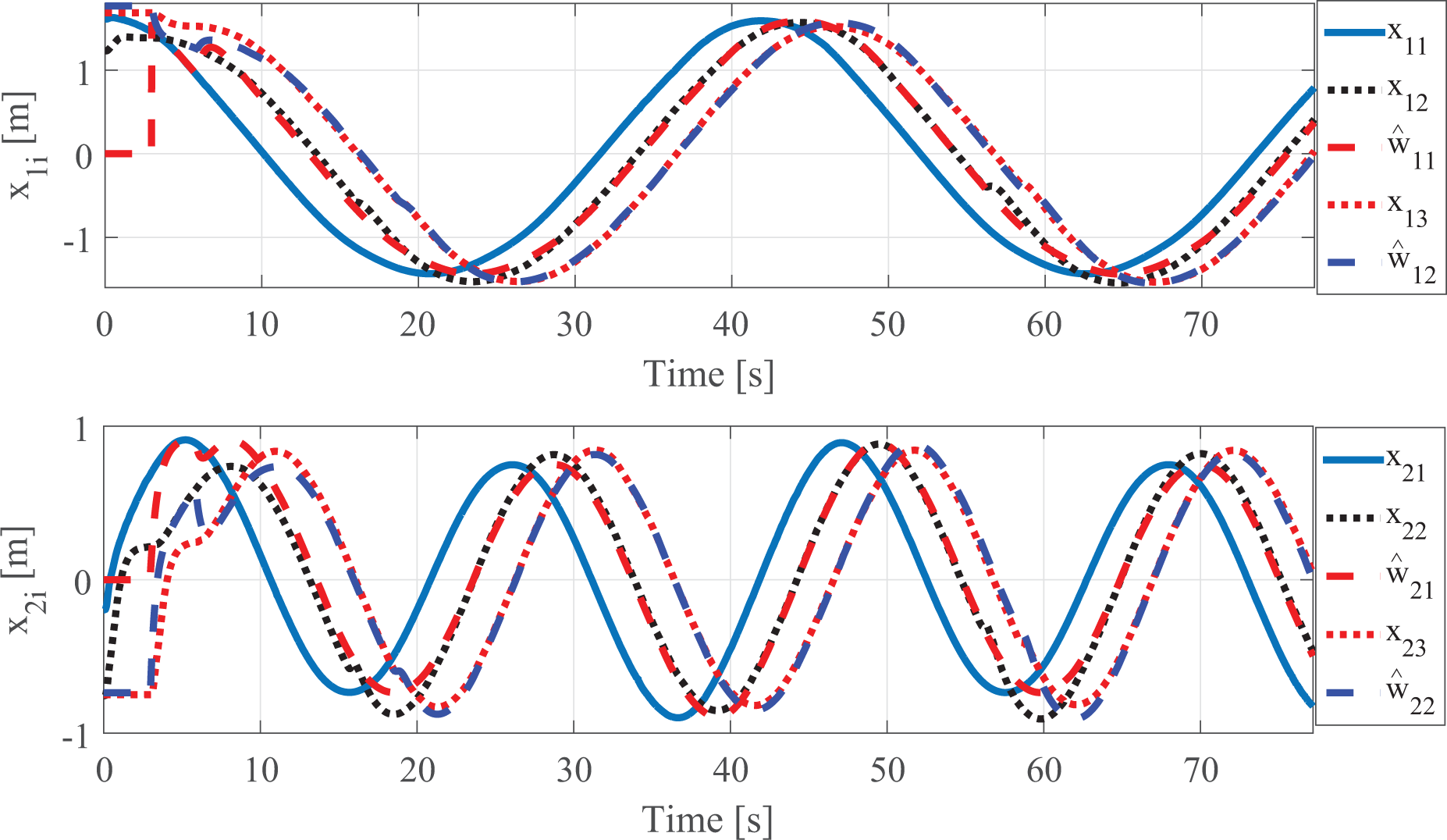
Robot x _1i, x _2i and observer ${\hat{w}}_{1 i}, {\hat{w}}_{2 i}$ positions with disturbances.

Figure 16.
Robots x _3i and observer ${\hat{w}}_{3 i}$ orientation angle with disturbances.

Figure 17 shows some snapshots of the experiment, where the sudden misplace of the second robot by a person is appreciated at 16th and 56th seconds, such that a turning of approximately 0.5 and 1.0 (rad) is induced at the robot orientation, respectively, see also Figure 16. Figure 18 shows the time evolution of the formation in the plane, showing that the disturbances take place at approximately coordinates (−0.5, −0.5) (m), such that the disturbance effects are appreciated at the left loop of the Lemniscata shape but are attenuated for the time the right loop is performed.

Figure 17.
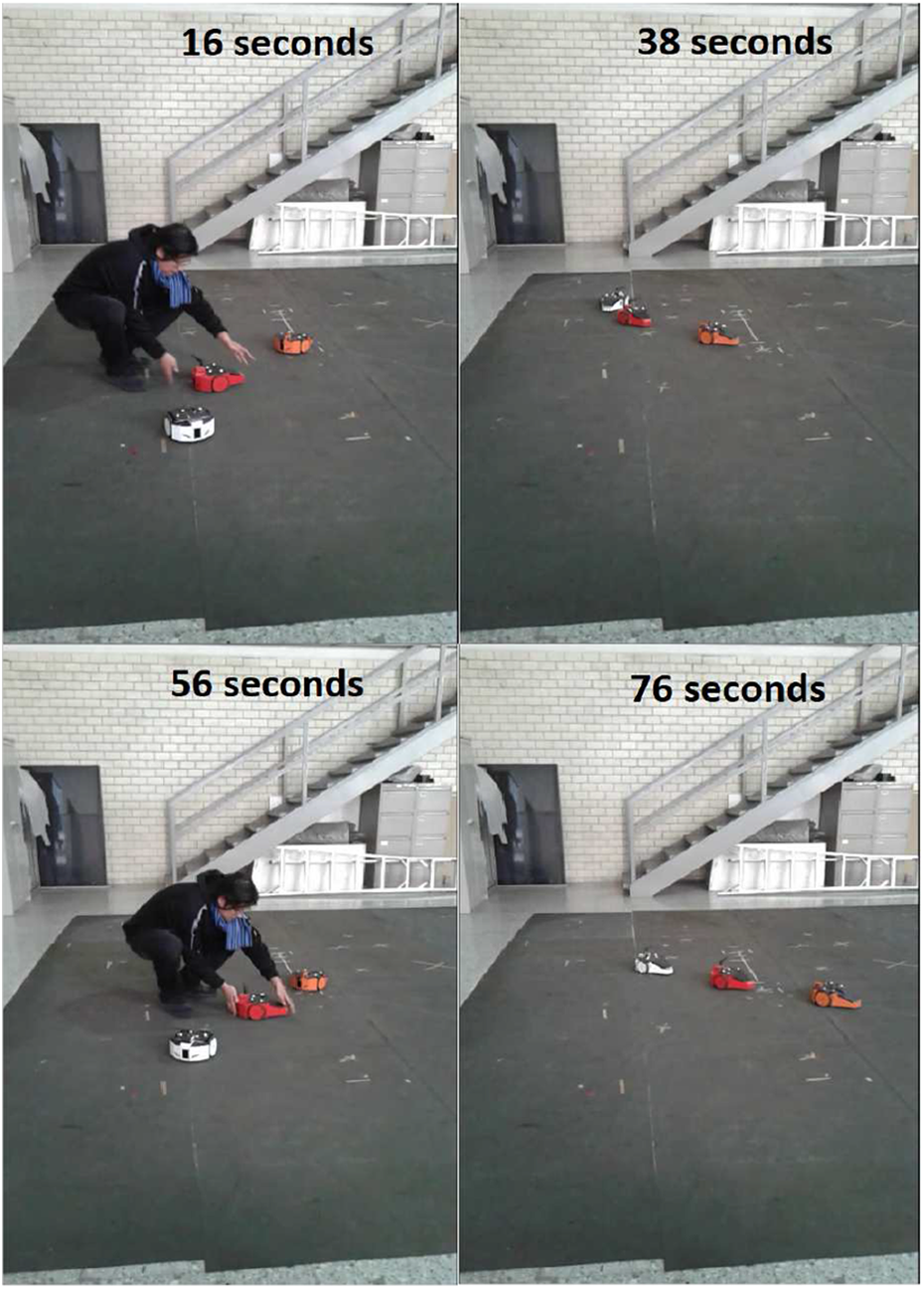
Real-time experiment with disturbances.

Figure 18.
Real-time experiment evolution of the platoon on the X–Y plane, with disturbances.

The observation errors $e_{w_{1 i}} (t), e_{w_{2 i}} (t), and e_{w_{3 i}} (t)$ are depicted in Figure 19, where their fast convergence is shown. The effect of the disturbances can also be observed in this figure. The tracking position errors $e_{s_{1 i}} (t), e_{s_{2 i}} (t)$ , and $e_{s_{3 i}} (t)$ are shown in Figure 20. Notice that although the effects of the two disturbances are evident, the tracking errors converge to zero as expected.

Figure 19.
Real-time experiment, observation errors with disturbances.

Figure 20.
Position tracking errors with disturbances.

In Figure 21, the control signals of the robots are shown. Notice how these signals change when the disturbances take place in the experiment, to compensate their effects and converge again to the formation. The behavior of the control signals is as expected by the theoretical results also, the signals shown the time-gap separation of τ units of time between them.

Figure 21.
Control signals evolution with disturbances.

Figure 22 shows how the separation or relative distance between the robots, d_i (t), behaves. The distance varies when the disturbance is introduced but after that it behaves as expected. It is important to notice that the numerical and real-time experiments have very similar behaviors between them, excluding the disturbances effects, despite the well-known differences between a simulation and the real-time experiment, such as model errors, friction forces, slipping phenomena, and mechanical issues of the robots, which are not considered on the kinematic model.

Figure 22.
Relative distance between robots with disturbances.

Conclusion

A platoon chain formation problem based on time-gap separation between any pair of consecutive robots in the formation, instead of a fixed distance, is considered in this work. The solution is based on a delay observer strategy that is able to provide the desired position and velocity references for each follower robot. The desired reference estimation is obtained by a position measurement assumption for each robot. The delay observer prevents the consideration of the usual dirty derivative and helps in the formal proof of the tracking error convergence. Numerical simulations and real-time experiments show the effectiveness of the proposed chain formation solution.

Robot	x _1i(m)	x _2i(m)	x _3i(rad)
Robot 1	1.55	−0.035	1.612
Observer 1	1.55	−0.035	1.612
Robot 2	1.76	−0.072	1.59
Observer 2	1.76	−0.072	1.59
Robot 3	1.98	−0.082	1.468

Robot	x _1i(m)	x _2i(m)	x _3i(rad)
Robot 1	1.61	−0.19	1.51
Observer 1	1.61	−0.19	1.51
Robot 2	1.23	−0.75	1.32
Observer 2	1.23	−0.75	1.32
Robot 3	1.68	−0.74	1.71

Footnotes

Declaration of conflicting interests

The author(s) declared no potential conflicts of interest with respect to the research, authorship, and/or publication of this article.

Funding

The author(s) disclosed receipt of the following financial support for the research, authorship, and/or publication of this article: This work was partially supported by the National Council for Science and Technology, CONACyT – Mexico, under the grant 254329.

References

Fax

Murray

. Information flow and cooperative control of vehicle formations. IEEE Trans Autom Control 2004; 49(9): 1465–1476.

Ren

Beard

. Distributed consensus in multi-vehicle cooperative control: Theory and applications. London: Springer, 2007.

Ren

Beard

Atkins

. Information consensus in multivehicle cooperative control. IEEE Contr Syst 2007; 27(2): 71–82.

Bai

Arcak

Wen

. Cooperative control design: A systematic, passivity-based approach. Springer Science & Business Media. New York: Springer-Verlag, 2011.

Consolini

Morbidi

Prattichizzo

. Leader–follower formation control of nonholonomic mobile robots with input constraints. Automatica 2008; 44(5): 1343–1349.

Zolotukhin

Kotov

Maltsev

. A relative measurement based leader-follower formation control of mobile robots. In: 12th international conference on informatics in control, automation and robotics (ICINCO), Colmar, Alsace, France, 21–23 July 2015, Vol. 02. pp. 310–313. IEEE.

Qian

Tong

. Leader-following formation control of multiple robots with uncertainties through sliding mode and nonlinear disturbance observer. ETRI J 2016; 38(5): 1008–1018.

Cruz-Morales

Velasco-Villa

Castro-Linares

. Leader-follower formation for nonholonomic mobile robots: discrete-time approach. Int J Adv Robot Syst 2016; 13(2): 46. DOI: 10.5772/62344.

Tanner

Pappas

Kumar

. Leader-to-formation stability. IEEE Trans Robot Autom 2004; 20(3): 443–455.

10.

Klanar

Matko

Blai

. Wheeled mobile robots control in a linear platoon. J Int Robot Syst 2009; 54(5): 709–731. DOI: 10.1007/s10846-008-9285-7.

11.

Peng

Wen

Rahmani

. Leader-follower formation control of nonholonomic mobile robots based on a bioinspired neurodynamic based approach. Robot Auton Syst 2013; 61(9): 988–996. DOI: 10.1016/j.robot.2013.05.004.

12.

Kowdiki

Barai

Bhattacharya

. Leader-follower formation control using artificial potential functions: a kinematic approach. In: IEEE-international conference on advances in engineering, science and management (ICAESM-2012), Nagapattinam, Tamil Nadu, India, 30–31 March 2012, pp. 500–505. IEEE.

13.

Guo

Lin

Cao

. Adaptive leader-follower formation control for autonomous mobile robots. In: Proceedings of the 2010 American control conference. pp. 6822–6827. DOI: 10.1109/ACC.2010.5531639.

14.

Qian

Tong

Guo

. Leader-follower-based formation control of nonholonomic mobile robots with mismatched uncertainties via integral sliding mode. Proc Instit Mech Eng I J Syst Control Eng 2015; 229(6): 559–569.

15.

Qian

Tong

. Integral sliding mode-based formation control of multiple uncertain robots via nonlinear disturbance observer. Int J Adv Robot Syst 2016; 13(6): 1–11. DOI: 10.1177/1729881416677694.

16.

Desai

Ostrowski

Kumar

. Controlling formations of multiple mobile robots. In: Proceedings. IEEE international conference on robotics and automation, Leuven, Belgium, Belgium, 20 May 1998, Vol. 4, pp. 2864–2869. IEEE.

17.

Gamage

Mann

GKI

Gosine

. Leader follower based formation control strategies for nonholonomic mobile robots: design, implementation and experimental validation. In: Proceedings of the 2010 American control conference. pp. 224–229. DOI: 10.1109/ACC2010.5530618.

18.

Dai

Lee

. The leader-follower formation control of nonholonomic mobile robots. Int J Control Autom Syst 2012; 10(2): 350–361.

19.

Chen

Sun

Yang

. A leader-follower formation control of multiple nonholonomic mobile robots incorporating receding-horizon scheme. Int J Robot Res 2009; 29: 727–747.

20.

Chen

Jia

. Adaptive leader-follower formation control of non-holonomic mobile robots using active vision. IET Control Theor Appl 2015; 9(8): 1302–1311. DOI: 10.1049/iet-cta.2014.0019.

21.

Low

. A flexible leader-follower formation tracking control design for nonholonomic tracked mobile robots with low-level velocities control systems. In: 2015 IEEE 18th international conference on intelligent transportation systems. pp. 2424–2431. DOI: 10.1109/ITSC.2015.391.

22.

Cristescu

Ionescu

Wyns

. Leader-follower string formation using cascade control for mobile robots. In: 2012 20th Mediterranean conference on control automation (MED). pp. 1092–1098. DOI: 10.1109/MED.2012.6265784.

23.

Klancar

Matko

Blazic

. A control strategy for platoons of differential drive wheeled mobile robot. Robot Auton Syst 2011; 59(2): 57–64. DOI: 10.1016/j.robot.2010.12.002.

24.

Marsden

McDonald

Brackstone

. Towards an understanding of adaptive cruise control. Trans Res C Emerg Technol 2001; 9(1): 33–51.

25.

Swaroop

Rajagopal

. A review of constant time headway policy for automatic vehicle following. In: ITSC 2001. 2001 IEEE intelligent transportation systems. Proceedings (Cat. No.01TH8585). pp. 65–69. DOI: 10.1109/ITSC.2001.948631.

26.

Liu

Goldsmith

Mahal

. Effects of communication delay on string stability in vehicle platoons. In: ITSC 2001. 2001 IEEE intelligent transportation systems. Proceedings (Cat. No.01TH8585). pp. 625–630. DOI: 10.1109/ITSC.2001.948732.

27.

Bareket

Fancher

Peng

. Methodology for assessing adaptive cruise control behavior. IEEE Trans Int Trans Syst 2003; 4(3): 123–131.

28.

Seppelt

Lee

. Making adaptive cruise control (acc) limits visible. Int J Human Comput Studies 2007; 65(3): 192–205.

29.

Milanes

Shladover

Spring

. Cooperative adaptive cruise control in real traffic situations. IEEE Trans Int Trans Syst 2014; 15(1): 296–305. DOI: 10.1109/TITS.2013.2278494.

30.

Ploeg

Semsar-Kazerooni

Lijster

. Graceful degradation of cooperative adaptive cruise control. IEEE Trans Int Trans Syst 2015; 16(1): 988 –996. DOI: 10.1109/TITS.2014.2349498.

31.

Wang

Barth

. Developing a distributed consensus-based cooperative adaptive cruise control system for heterogeneous vehicles with predecessor following topology. J Adv Trans 2017; 2017: 1–16. DOI: 10.1155/2017/1023654.

32.

Canudas de Wit

Siciliano

Bastin

. Theory of robot control. London: Springer-Verlag, 1996.

33.

d’Andrèa Novel

Campion

Bastin

. Control of nonholonomic wheeled mobile robots by state feedback linearization. Int J Robot Res 1995; 14(6): 543–559. DOI: 10.1177/027836499501400602.

34.

Khalil

. Nonlinear systems. New Jersey: Prentice-Hall, 1996.

Chain formation control for a platoon of robots using time-gap separation

Abstract

Keywords

Introduction

Kinematic model and problem formulation

Problem formulation

Input delay observer design

Assumption 1

Assumption 2

Remark 3

Observation error analysis

Lemma 4

Proof

Remark 5

Remark 6

Observer-based time-gap platoon formation strategy

Remark 7

Tracking error convergence

Lemma 8

Proof

Remark 9

Platoon chain formation strategy evaluation

Numerical evaluation

Real-time experiments

Experimental platform

Experimental results without disturbances

Experimental results with disturbances

Conclusion

Footnotes

Declaration of conflicting interests

Funding

References