Sage Journals: Discover world-class research

Abstract

To address the localization problem for a mobile robot in an indoor environment, an improved visual localization system based on artificial markers is proposed in this article. First, we will present a novel artificial marker which can be detected and identified easily and correctly. We will then introduce how it is designed, recognized, and verified. The markers are arranged on the ceiling and the mobile robot moves around on the ground to capture images with an up-facing monocular camera. The markers’ information, including the position and direction, will be obtained by processing the images. The camera’s uncertainty model is then put forward based on the distortion of the camera. The uncertainty of the obtained markers’ information is analyzed through the uncertainty model. Finally, with the obtained information, the marker map in global image coordinate system is established and optimized through a graph-based algorithm in which the edges can be updated to reduce the uncertainty using Bayes Estimation method. To verify the effectiveness of the localization system, numerous experiments have been conducted. Additionally, the proposed method has also been applied to industrial forklift to test its robustness in a factory environment.

Keywords

Visual localization ceiling-based location artificial marker SLAM G2O

Introduction

In the field of mobile robotics, self-localization is one of the most challenging issues, particularly in dynamic environments. Due to an extensive and wide range of solutions, the localization problem has always been widely investigated in autonomous robotics.^1

–4 During the last few decades, many kinds of techniques and methods have been developed with varying levels of acceptance, such as dead reckoning based on an odometer,⁵ algorithms based on wireless sensor networks,⁶ inertial sensor-based algorithms,⁷ and map-matching algorithms based on vision.⁸

Among all available sensors, cameras have been increasingly applied to vision-based mobile robot localization due to their low prices, ease of use, and ability to offer abundant information. Generally, the information of the environment could be extracted from the captured image and utilized to determine the position and orientation of a mobile robot through visual positioning method. Recently, the vision-based simultaneous localization and mapping (VSLAM) approach has drawn a lot of attention in the mobile robotics field. And it can give an autonomous robot the abilities to explore an unknown environment and localize itself while building a reliable map. Several visual simultaneous localization and mapping (SLAM) systems have been developed and widely used in application,⁹ including the MonoSLAM,¹⁰ the PTAM,¹¹ the FrameSLAM,¹² or the systems based on the G2O framework.¹³ Most of them use the features of environment^14
–16 and are usually carried out using natural or artificial markers. It is difficult to detect and compare the natural features of a noisy environment. In contrast, the detection of artificial markers is much easier, as they are designed with a predetermined color, size, and shape. Therefore, artificial markers are commonly used for navigation and map building in indoor environments.^17,18 They can increase the accuracy of localization for vision-based mobile robot guidance systems.

Artificial marker-based localization systems have been developed in recent years.¹⁹ Wen et al.²⁰ designed a ceiling- or wall-attached landmark that is pentagonal and identified by binary BCH code.²¹ It located a mobile robot based on the homography between the landmark plane and the image plane. The average robot’s speed could reach 0.18 m/s. Wu et al.²² designed new artificial landmark based on QR code technology and proposed a localization algorithm based on vanishing line principle. Okuyama et al.²³ achieved positioning of a mobile robot through the VSLAM technique based on the newly developed artificial markers. Based on artificial landmarks, Aleksandrovich et al.²⁴ developed a machine vision system, which identified artificial landmarks on images from a video camera with pan–tilt mechanism and could eliminate course deviation calculated on the basis of information about artificial landmarks. To reduce the interference of illumination variation, visual localization approaches based on infrared markers have been attracting more attention.^25,26 Ren et al.²⁷ realized the localization of the robot using light-emitting diodes as artificial landmarks. Sultan et al.²⁸ designed a kind of artificial marker based on an infrared dot matrix and presented the corresponding algorithm to identify the marker. Zhou et al.²⁹ provided an embedded visual localization system composed of an infrared-reflective artificial marker pasted on the ceiling and an image acquisition and processing unit installed on the robot. This method calculated the position of the robot through Perspective-3-Points algorithm.

In this article, we propose a novel localization system based on the newly designed markers. The marker, which should be attached on the ceiling, can be recognized and identified correctly with high speed. There is no strict requirement for the arrangement of the markers. When the robot moves around on the ground with an up-facing camera, the system learns the distribution of the markers and builds a corresponding marker map in the image coordinate. The position of the robot can then be calculated through the map. In addition, the G2O framework is used to further optimize the accuracy of the marker map. And, the camera’s uncertainty model is also built based on the camera distortion, which could be used to update the edges in G2O framework. The new system has been evaluated through experimentation and the results show that it can meet the industrial requirements in localization accuracy and frequency.

The article is organized as follows. In the next section, we will present the new artificial marker and introduce how it is recognized and verified. The uncertain model of the camera is defined in the third section. The localization system is described in the section “Multi-marker based visual localization system”. In the section “Experiments and results”, experiments are conducted and the results are presented.

Design and recognition of artificial markers

For convenient localization, an artificial marker should have a special identity (ID) and directionality. The markers are also required to be easily and reliably detected and identified. To improve the real-time performance in the localization system, the markers’ information should be extracted and recognized quickly and correctly. This part will introduce a new kind of artificial marker which can meet all these requirements. It also offers a robust marker recognition algorithm, which sufficiently considers the external disturbance, such as the varying illumination conditions and image blurring which may be caused by the robot’s movement.

Design of artificial markers

In our design, an artificial marker is a planar square pattern consisting of a set of small squares which could be encoded. The outer part can isolate the marker from the background. If the background is a dark color such as black, the outer part could be a light color such as white and vice versa. In this article, we use two colors which can form a strong contrast to encode the ID of the marker. For example, in factory experiments, the ceiling’s color is dark gray, so we use the white on the outer. For the inner part, a white square represents 0, while a black square represents 1. Unless otherwise stated, we will take this marker as the default in the following part.

The four parts V1–V4 can indicate the direction of the marker by coloring V1 black and the rest white. The marker is encoded with 12 binary hamming codes of which C1–C4 are parity bits and D1–D8 are data bits. The marker we will use has eight data bits, and the total useful number of IDs is 2⁸ − 1=255, which could cover 140,000 m² in area. We present the ID number in binary, and D1 denotes the lowest bit while D8 indicates the highest bit. As is shown in Table 1, the parity bits are associated with the data bits. From the table, we can see that the parity bits C1–C4 are only associated with themselves and can represent each different binary bit position. It means that C1–C4 indicate the first, second, third, and fourth bit of the binary bit position from the left, respectively. The other data bits D1–D8 are associated with them according to their bit position in binary form. Then, we will set each of the parity bits to be a certain data to make sure that they and their associated data bits can satisfy the parity check rule which, for example, can be as equation (2). For example, the left first bit of the binary bit position of D1, D3, D4, D5, and D7 is one, so, they are associated with C1. When we use the odd parity check, the parity check rule is set to be as

D 7 \oplus D 5 \oplus D 4 \oplus D 2 \oplus D 1 \oplus C 1 = 1

Table 1.

The relationship between data bits and parity bits.

Bit position		1	2	3	4	5	6	7	8	9	10	11	12
Bit position in binary form		0001	0010	0011	0100	0101	0110	0111	1000	1001	1010	1011	1100
Encoded data bits		C1	C2	D1	C3	D2	D3	D4	C4	D5	D6	D7	D8
Parity Bit coverage	C1	×		×		×		×		×		×
	C2		×	×			×	×			×	×
	C3				×	×	×	×					×
	C4								×	×	×	×	×

× means that they are associated.

where the operator ⊕ means nonequivalence operation. If any one of D1, D3, D4, D5, and D7 are wrongly detected, the rule cannot be met.

In this way, the number of C1–C4 could be calculated by the following formulas

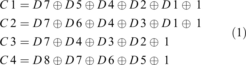
\begin{array}{l} C 1 = D 7 \oplus D 5 \oplus D 4 \oplus D 2 \oplus D 1 \oplus 1 \\ C 2 = D 7 \oplus D 6 \oplus D 4 \oplus D 3 \oplus D 1 \oplus 1 \\ C 3 = D 7 \oplus D 4 \oplus D 3 \oplus D 2 \oplus 1 \\ C 4 = D 8 \oplus D 7 \oplus D 6 \oplus D 5 \oplus 1 \end{array}

When the marker is encoded in the way described above, we could get the 12 binary data bits associated with the inner part. Then, we color the squares with black when the corresponding data bit is 1, while others are kept white. For example, the ID number of Figure 1(c) is 1. The outer contour of the outer part has four vertices, P1–P4. P1, which is nearest to the V1 part, is defined as the origin point. The direction of X-axis is the same with the vector $\vec{P 1 P 2}$ , while the direction of Y-axis is pointing from P1 to P4. Figure 1(b) indicates proportional relation among all the parts in size.

Figure 1.

Design of the artificial marker.

The size of the marker is determined based on the height of the ceiling. The higher the ceiling is, the larger the marker should be. There is no strict requirement of the size. But it would be better if the size of the marker’s edge was more than 80 pixels long.

Extraction and recognition of the marker

In this process, we can get the marker’s ID, origin point, and direction information in the image. The markers are identified in three main steps: (1) marker extraction, which offers the marker candidates; (2) marker verification, which identifies the marker from the candidates; (3) information acquisition, including the ID number, the position, and the direction information of the marker.

Marker detection: In this step, the image is analyzed in order to find square shapes that are candidates to be markers. First, we convert the captured color image into a grayscale image and turn it into a black-and-white image through the method of adaptive thresholding. For each pixel in the image, the threshold value is set to be the weighted sum of neighborhood values, where weights are a Gaussian Window. If the pixel value is below the threshold value, it is set to the background value; otherwise, it is set to be the foreground value. Then, the contours are extracted from the threshold image and those which are not convex or not approximate to a square shape are abandoned. Some extra filtering processes are also applied to remove contours that are too small or too big or too close to each other. Finally, four vertices of the remaining contours are obtained, which will be used in the next step.

Marker verification: After marker detection, it is necessary to judge if they are real markers or not by analyzing their coding parts. This step involves extracting the data bits of each marker. To do so, firstly, perspective transformation is applied to obtain the marker in canonical form. The canonical image is binary processed with Otsu and divided into different parts according to the marker size as shown in Figure 2(e). The proportion of black or white pixels in each part is calculated to determine whether it is a white or a black bit. Then, 16 data bits corresponding to the 16 parts of the marker are extracted from the image. In addition, the 12 pieces of inner data can be used to determine whether the ID is valid. If the candidate is a true marker, the conditions below should be satisfied

\begin{array}{l} D 7 \oplus D 5 \oplus D 4 \oplus D 2 \oplus D 1 \oplus C 1 = 1 \\ D 7 \oplus D 6 \oplus D 4 \oplus D 3 \oplus D 1 \oplus C 2 = 1 \\ D 7 \oplus D 4 \oplus D 3 \oplus D 2 \oplus C 3 = 1 \\ D 8 \oplus D 7 \oplus D 6 \oplus D 5 \oplus C 4 = 1 \end{array}

When the equations cannot be satisfied, the marker is not valid or wrongly recognized.

Information acquisition: After marker verification, we can calculate the marker ID according to the weight matrix of the marker circles

ID = W \cdot Q

where

W = {[\begin{array}{l} D 1 \\ D 2 \\ D 8 \\ D 4 \\ D 5 \\ D 6 \\ D 7 \\ D 8 \end{array}]}^{T} Q = [\begin{array}{l} 0 x 01 \\ 0 x 02 \\ 0 x 04 \\ 0 x 08 \\ 0 x 10 \\ 0 x 20 \\ 0 x 40 \\ 0 x 80 \end{array}]

Figure 2.

The steps of the marker detector.

As shown in Figure 3, the marker coordinate system XOY is established in the current image plane X′O′Y′. The direction of vector $\vec{O P_{2}}$ corresponds to the X-axis. The direction information can be acquired through the following formulas

α = {\begin{cases} - arccos (\frac{p_{2 x} - p_{1 x}}{\sqrt{{(p_{2 x} - p_{1 x})}^{2} + {(p_{2 y} - p_{1 y})}^{2}}}) if p_{2 y} < p_{1 y} \\ arccos (\frac{p_{2 x} - p_{1 x}}{\sqrt{{(p_{2 x} - p_{1 x})}^{2} + {(p_{2 y} - p_{1 y})}^{2}}}) if p_{2 y} < p_{1 y} \end{cases}

Figure 3.

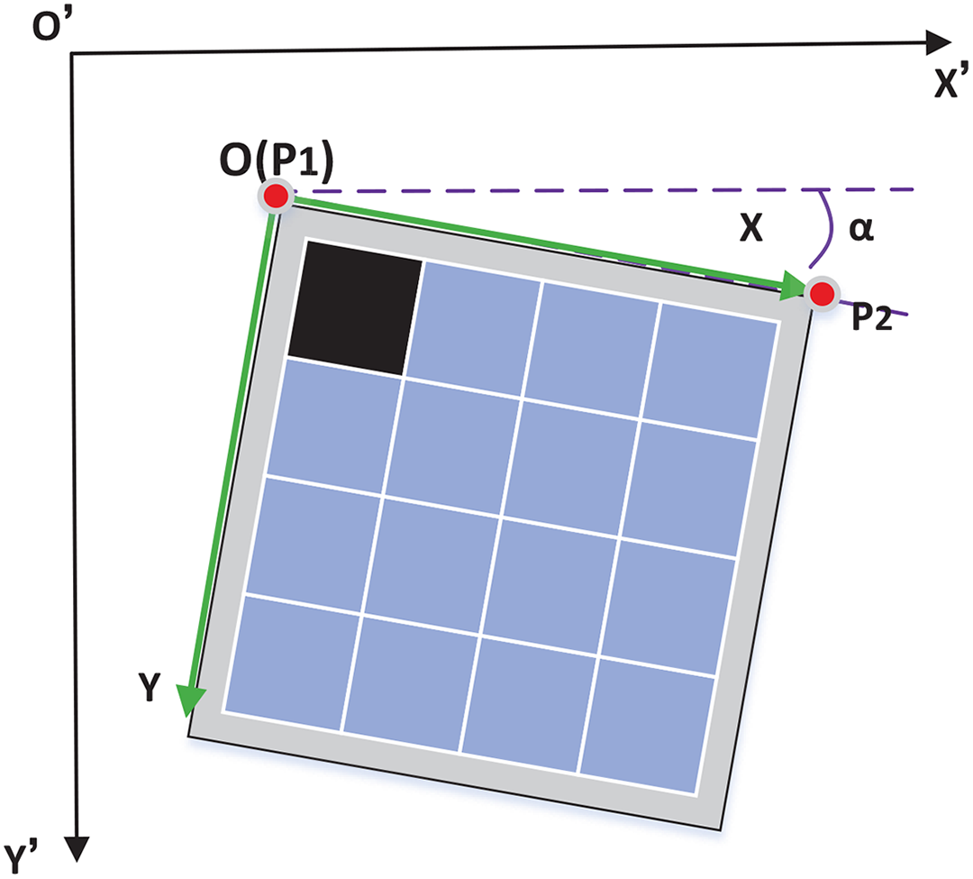
The relationship between the marker’s coordinate and the image frame.

The uncertainty model of the camera

Because of the distortion of the camera, the information we directly get from the captured image is not accurate. Usually, we correct the image before processing it. However, this is complex and time-consuming. In this article, we denote the information by the obtained data and a corresponding variance. In this section, we proposed an uncertainty model of the camera according to its distortion.

As we know, the relationship between the world coordinate system and the camera coordinate system can be described as

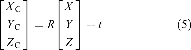
[\begin{matrix} X_{C} \\ Y_{C} \\ Z_{C} \end{matrix}] = R [\begin{matrix} X \\ Y \\ Z \end{matrix}] + t

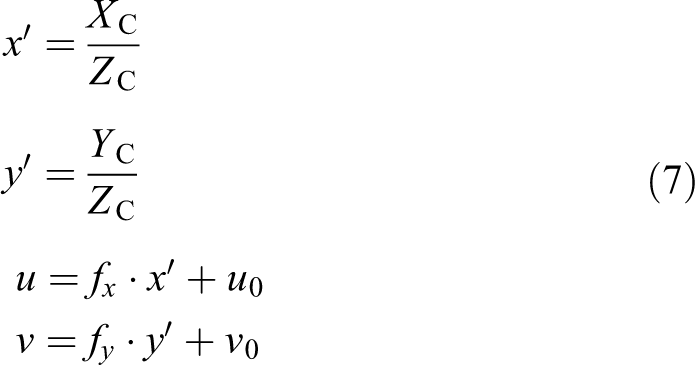
where $(X, Y, Z)$ and $(X_{C}, Y_{C}, Z_{C})$ represent the coordinates of a 3-D point in the world coordinate space and the camera coordinate system, respectively. R means the rotation matrix and t indicates the translation matrix.

The transform relationship between the physics camera coordinate system and the pixel coordinate system is presented as follows

Z_{C} \cdot [\begin{matrix} u \\ v \\ 1 \end{matrix}] = A \cdot [\begin{matrix} X_{C} \\ Y_{C} \\ Z_{C} \end{matrix}]

where $(u, v)$ is the coordinates of the projection in pixels. A is a matrix of intrinsic parameters

A = [\begin{matrix} f_{x} & 0 & u_{0} \\ 0 & f_{y} & v_{0} \\ 0 & 0 & 1 \end{matrix}]

where $(u_{0}, v_{0})$ indicates the principal point which is usually at the image center. $f_{x} and f_{y}$ are the local length and they are commonly equal.

Then, we can get

\begin{array}{l} x^{'} = \frac{X_{C}}{Z_{C}} \\ y^{'} = \frac{Y_{C}}{Z_{C}} \\ u = f_{x} \cdot x^{'} + u_{0} \\ v = f_{y} \cdot y^{'} + v_{0} \end{array}

However, there exists some distortion in the camera lens, including the radial distortion and tangential distortion. The tangential distortion can be ignored, because it is very small relative to the lateral distortion. Then, the pinhole camera model has been extended as follows

\begin{array}{l} x^{'} = \frac{X_{C}}{Z_{C}} \\ y^{'} = \frac{Y_{C}}{Z_{C}} \\ x^{''} = x^{'} (1 + k_{1} r^{2} + k_{2} r^{4}) \\ y^{''} = y^{'} (1 + k_{1} r^{2} + k_{2} r^{4}) \\ u^{'} = f_{x} \cdot x^{''} + u_{0} \\ v^{'} = f_{y} \cdot y^{''} + v_{0} \end{array}

where $k_{1} and k_{2}$ are radial distortion coefficients and $r = \sqrt{x^{' 2} + y^{' 2}}$ .

The model of radial nonlinear distortion of the camera can be described as

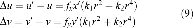
\begin{array}{l} Δ u = u^{'} - u = f_{x} x^{'} (k_{1} r^{2} + k_{2} r^{4}) \\ Δ v = v^{'} - v = f_{y} y^{'} (k_{1} r^{2} + k_{2} r^{4}) \end{array}

From equation (9), we can know that the uncertainty of one pixel gets bigger when its distance to the image center gets longer, and their relationship is nonlinear.

For a Gaussian distribution $P : N (μ, σ^{2})$ , the probability of the numerical distribution in $[μ - 3 σ, μ + 3 σ]$ is 0.9974. This principle is called 3σ rule. Usually, the range of a point’s variance is within its distortion. For a point $P (x, y)$ , the value of x is supposed to be in $[x - Δ u, x + Δ u]$ , and the value of y is in $[y - Δ v, y + Δ v]$ . We assume that $P : N (μ, σ^{2})$ , where $μ = {[\begin{matrix} x & y \end{matrix}]}^{T}$ and $σ = {[\begin{matrix} σ_{x} & σ_{y} \end{matrix}]}^{T}$ . According to the rule, the variance of point is defined as follows

\begin{array}{l} σ_{x} = \frac{Δ u}{3} \\ σ_{y} = \frac{Δ v}{3} \end{array}

For a vector, such as $\vec{P_{1} P_{2}}$ , we define $\vec{P_{1} P_{2}} : N (Δ μ, Δ σ^{2})$ , where

\begin{array}{l} Δ μ = {[x_{P 2} - x_{P 1} y_{P 2} - y_{P 1}]}^{T} \\ Δ σ = {[δ σ_{x} δ σ_{y}]}^{T} = [σ_{P 1 x} + σ_{P 2 x} σ_{P 1 y} + σ_{P 2 y}] \end{array}

We define θ as an angle which indicates the direction of vector $\vec{P_{1} P_{2}}$ in the image frame. From Figure 4, we can see that θ has a varying range denoted by dθ. Then we transfer the variance of P₁ to P₂, and the result is shown in Figure 4(b). Due to $L ≫ 6 σ_{P 1} + 6 σ_{P 2}$ , we can get

d θ = arcsin \frac{6 σ_{P 1} + 6 σ_{P 2}}{L}

Figure 4.

The process to estimate the variance of θ.

where

\begin{array}{l} θ_{P 1} = \sqrt{{(σ_{P 1 x}^{2} + σ_{P 1 y}^{2})}^{2}} \\ θ_{P 2} = \sqrt{{(σ_{P 2 x}^{2} + σ_{P 2 y}^{2})}^{2}} \\ L = \sqrt{{(x_{P 1} - x_{P 2})}^{2} + {(y_{P 1} - y_{P 2})}^{2}} \end{array}

Then, according to the 3σ rule, the variance of θ is as follows

σ_{θ} = \frac{d θ}{6} = \frac{1}{6} arcsin \frac{6 σ_{P 1} + 6 σ_{P 2}}{L} =arcsin \frac{σ_{P 1} + σ_{P 2}}{L}

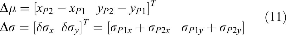
The difference of two angles θ₁ and θ₂ whose variance are $σ_{θ 1}$ and $σ_{θ 2}$ , respectively, is

Δ θ = θ_{1} - θ_{2}

And the variance of Δθ can be calculated as

Δ σ_{θ} = σ_{θ 1} + σ_{θ 2}

In this article, Δσ and $Δ σ_{θ}$ are used to describe the covariance of the relationship between two markers in an image.

Multi-marker-based visual localization system

To realize the localization indoors, the newly designed markers are fixed to the ceiling, while the mobile robot moves around with an up-facing camera on top of it for image capturing. In this article, we regard the camera’s location as the robot’s location and use SLAM technology for localization. As we know, once the markers are arranged, their locations are normally unchanged. On that basis, we have put forward a newly designed localization system which can simplify the traditional SLAM method. As shown in Figure 5, the system only builds the marker map in global image coordinate. And the graph-based algorithm with G2O framework is used to optimize the marker map. Here, the markers’ positions indicate the nodes, and the relations between different markers represent the edges of the graph. Besides, in order to increase the positioning accuracy, an uncertainty model is proposed to take the influence of the camera’s distortion into account.

Figure 5.

The flow chart of the localization system.

Parameter determination and coordinates establishment

For the indoor mobile robot working in planar floor, there are only the motions moving along $X_{ω}$ - and $Y_{ω}$ -axes and rotating around $Z_{ω}$ -axis. Usually, the ceiling is parallel to the floor, which simplifies the imaging geometric relationship as follows

[\begin{matrix} k u_{d i} \\ k v_{d i} \\ 1 \end{matrix}] = [\begin{matrix} cos φ_{i} & - sin φ_{i} & p_{x i} \\ sin φ_{i} & cos φ_{i} & p_{y i} \\ 0 & 0 & 1 \end{matrix}] [\begin{matrix} x_{w i} \\ y_{w i} \\ 1 \end{matrix}]

where $(x_{w i}, y_{w i})$ and $(u_{d i}, v_{d i})$ represent the coordinates of a point P_i on the ceiling in the world frame and the ith sampled image frame, respectively, $u_{d i} = u_{i} - u_{0}, v_{d i} = v_{i} - v_{0}$ . $(p_{x i}, p_{y i})$ denotes the position of the world frame relative to the camera coordinate at the ith sample. φ_i represents the robot’s direction when sampled. k is the scale factor between the image space and the Cartesian space. We can get k with the distance of two points on the ceiling in world coordinate frame and the number of pixels between them in the image frame.

Above all, we define $X_{f}^{n} O_{f}^{n} Y_{f}^{n}$ to be the coordinate system of the nth captured image frame. $X_{C}^{n} O_{C}^{n} Y_{C}^{n}$ is the coordinate system attached to the center of the camera. Its origin coincides with the current image center and its direction is the same with $X_{f}^{n} O_{f}^{n} Y_{f}^{n}$ . When the first marker is detected, the current image’s coordinate frame is defined to be $X_{f}^{0} O_{f}^{0} Y_{f}^{0}$ and the camera’s coordinate is $X_{C}^{0} O_{C}^{0} Y_{C}^{0}$ . In the frame $X_{f}^{0} O_{f}^{0} Y_{f}^{0}$ , both the global image coordinate system $X_{I} O_{I} Y_{I}$ and the real-world coordinate system $X_{W} O_{W} Y_{W}$ are determined, and their origins and directions are the same with $X_{C}^{0} O_{C}^{0} Y_{C}^{0}$ , as shown in Figure 6. Meanwhile, $X_{m i} O_{m i} Y_{m i}$ means the ith detected marker’s coordinate frame. The scales of $X_{W} O_{W} Y_{W}$ and $X_{I} O_{I} Y_{I}$ have a proportional relationship which is denoted by k in both X- and Y-axis directions. Then, the position and direction of $X_{m 0} O_{m 0} Y_{m 0}$ can be calculated in the current image frame $X_{f}^{n} O_{f}^{n} Y_{f}^{n}$ , as well as in the $X_{I} O_{I} Y_{I}$ .

Figure 6.

The establishment of the coordinate systems.

After the coordinates are established, the first detected marker is added to the marker map. When a new marker is detected, there should be another marker, which is already in the marker map, in the same image. In this way, the initial position of the newly detected marker can be calculated and then it is added to the marker map.

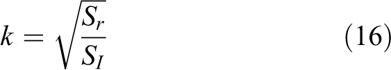
The coefficient k can be calculated when the first marker is detected in the obtained image. As the actual size of the marker is known, we can easily get its area S_r in square millimeter. When the image is processed, the marker’s area S_I in pixels can be obtained. Then, k can be calculated as follows

k = \sqrt{\frac{S_{r}}{S_{I}}}

Graph-based optimization

To improve the quality of the marker map, a graph-based optimization algorithm is proposed. Once the global image coordinate system is established, the marker map in it can be built. The positions of markers are set to be the nodes of the graph, while the relative location relationships between each pair of the markers form the edges or constraints of the graph. Usually, there exist several edges between each two markers, because they can be seen from different points of view. However, the calculating time of the algorithm is proportional to the number of edges. It is too time-consuming for real-time application. But if we randomly choose one edge which may have a larger error, then an inaccurate marker map will be generated. Here, we propose a new method which can keep one edge between each two nodes while taking into consideration of all the edge information and calculate the edges using the Bayes Parameter Estimation method.

As shown in Figure 7, the position and direction of $X_{m i} O_{m i} Y_{m i}$ are set to be the nodes, and the relative relationships ${edge}_{i j}$ indicate the edges of the graph. The edge information is described by the measured value, and a related variance which can be obtained from the camera’s uncertainty model

{edge}_{i j} : N (Δ r_{i j}, Δ σ_{i j}^{2})

Figure 7.

The building of the marker map through the graph-based method.

where

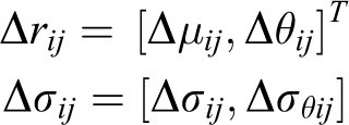
\begin{matrix} Δ r_{i j} = {[Δ μ_{i j}, Δ θ_{i j}]}^{T} \\ Δ σ_{i j} = [Δ σ_{i j}, Δ σ_{θ i j}] \end{matrix}

When we acquire another piece of information on the same edge presented by the measured data and uncertainty ${edge}_{i j}^{'} : N (Δ r_{i j}^{'}, Δ σ_{i j}^{' 2})$ , the corresponding edge can be updated using the Bayes Parameter Estimation method and written as follows

\begin{matrix} Δ r_{i j} = \frac{Δ r_{i j} Δ σ_{i j}^{2} + Δ r_{i j}^{'} Δ σ_{i j}^{' 2}}{Δ σ_{i j}^{2} + Δ σ_{i j}^{' 2}} \\ Δ σ_{i j} = \frac{Δ σ_{i j}^{2} Δ σ_{i j}^{' 2}}{Δ σ_{r i j}^{2} + Δ σ_{i j}^{' 2}} \end{matrix}

In this method, we update the edges when new data are acquired, instead of adding all the edges into the formulation. This will lead to reduction of the processing time and improved accuracy of the marker map.

With the updated edges, the graph-based optimization can be done in the next process. Pose graph is very convenient and intuitive to represent the relative position between different markers in global image coordinate system. In general, graph optimization is a nonlinear optimization problem, where each node represents the parameter (marker’s pose) to be optimized, and each edge represents the constraint. Let $X = (X_{1}, X_{2}, \dots, X_{n})^{T}$ be a vector of parameters that describes the configuration of the nodes. $ω_{i j}$ and $Ω_{i j}$ are defined as the mean and the information matrix of the observation value between node j and node i, respectively. Given the state X, $f_{i j} (X)$ is a function that calculates the perfect observation according to the current state. Then, the residual e_ij can be calculated by

e_{i j} (X) = ω_{i j} - f_{i j} (X)

The amount of errors introduced by each constraint weighed by its information matrix can be calculated by

d_{i j} {(X)}^{2} = e_{i j} {(X)}^{T} Ω_{i j} e_{i j} (X)

Therefore, assuming all of the constraints to be independent, the overall error is

D^{2} (X) = \sum d_{i j} {(X)}^{2} = \sum e_{i j} {(X)}^{T} Ω_{i j} e_{i j} (X)

Ultimately, each marker pose can be estimated by minimizing the cost function, and the solution to the graph-SLAM problem is to find a state $x^{*}$ that minimizes the overall error

X^{*} = \underset{X^{*}}{argmin} \sum_{i j} e_{i j}^{T} Ω_{i j} e_{i j}

In our system, each marker’s pose and observation constraint is defined as

\begin{array}{l} X^{T} = (t_{i}^{T}, θ_{i}) \\ Z_{i j}^{T} = (t_{i j}^{T}, θ_{i j}) \end{array}

and

ω_{i j} = μ_{i j}

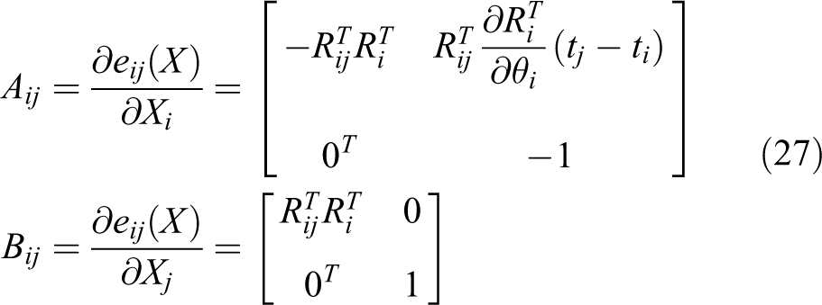
where t_i denotes the marker’s position ${(x_{i}, y_{i})}^{T}$ and t_ij denotes the relative position of the two markers. θ_i indicates the marker’s direction and $θ_{i j}$ is the difference between the directions of the two markers, whose range is $[- π, π]$ . $Z_{i j}^{T}$ indicates the relative posture between the ith marker and the jth marker.

The error function could be expressed by

e_{i j} (X) = [\begin{matrix} R_{i j}^{T} (R_{i}^{T} (t_{j} - t_{i}) - t_{i j}) \\ θ_{j} - θ_{i} - θ_{i j} \end{matrix}]

where R_i is a 2 × 2 rotation matrix. It can be written as

R_{i} = [\begin{array}{l} cos (θ_{i}) & - sin (θ_{i}) \\ sin (θ_{i}) & cos (θ_{i}) \end{array}]

The corresponding error function Jacobian matrix is

\begin{array}{l} A_{i j} = \frac{\partial e_{i j} (X)}{\partial X_{i}} = [\begin{matrix} - R_{i j}^{T} R_{i}^{T} & R_{i j}^{T} \frac{\partial R_{i}^{T}}{\partial θ_{i}} (t_{j} - t_{i}) \\ 0^{T} & - 1 \end{matrix}] \\ B_{i j} = \frac{\partial e_{i j} (X)}{\partial X_{j}} = [\begin{matrix} R_{i j}^{T} R_{i}^{T} & 0 \\ 0^{T} & 1 \end{matrix}] \end{array}

Iterative approaches such as Gauss–Newton or Levenberg–Marquadt can be used to compute the optimal state estimate. G2O is an open-source C++ framework for optimizing graph-based nonlinear error functions, such as equation (25) in our method. It is usually used to find the configuration of parameters or state variables that maximally explains a set of measurements affected by Gaussian noise. G2O has been designed to be easily extensible to a wide range of problems, and a new problem typically can be specified within a few lines of code. The marker map is built as a graph, and it can be optimized using the G2O framework. After an optimization iteration, the positions of the markers in the map are modified. Once a new marker is added or the edge is updated, the graph will be optimized.

Localization

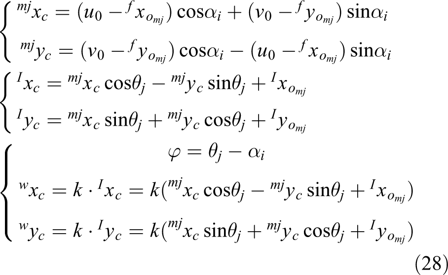
During the period of marker map establishment in global image coordinates, the robot can calculate its position at the same time. Figure 8 shows a sampled moment when the jth marker is viewed and the positioning process is shown below

\begin{array}{l} {\begin{cases} ^{m j} x_{c} = (u_{0} - {}^{f}x_{o_{m j}}) cos α_{i} + (v_{0} - {}^{f}y_{o_{m j}}) sin α_{i} \\ ^{m j} y_{c} = (v_{0} - {}^{f}y_{o_{m j}}) cos α_{i} - (u_{0} - {}^{f}x_{o_{m j}}) sin α_{i} \end{cases} \\ {\begin{cases} ^{I} x_{c} = {}^{m j}x_{c} cos θ_{j} - {}^{m j}y_{c} sin θ_{j} + {}^{I}x_{o_{m j}} \\ ^{I} y_{c} = {}^{m j}x_{c} sin θ_{j} + {}^{m j}y_{c} cos θ_{j} + {}^{I}y_{o_{m j}} \end{cases} \\ {\begin{matrix} φ = θ_{j} - α_{i} \\ ^{w} x_{c} = k \cdot {}^{I}x_{c} = k (^{m j} x_{c} cos θ_{j} - {}^{m j}y_{c} sin θ_{j} + {}^{I}x_{o_{m j}}) \\ ^{w} y_{c} = k \cdot {}^{I}y_{c} = k (^{m j} x_{c} sin θ_{j} + {}^{m j}y_{c} cos θ_{j} + {}^{I}y_{o_{m j}}) \end{matrix} \end{array}

Figure 8.

Part of the marker map and its relationship with the current image frame at a sampled moment.

where $(^{m j} x_{c},^{m j} y_{c})$ and $(^{I} x_{c},^{I} y_{c})$ indicate the coordinates of the current picture’s center point $(u_{0}, v_{0})$ in the jth marker’s frame and the global image frame, respectively. $(^{w} x_{c},^{w} y_{c}, φ)$ represents the position and orientation information of the robot in the world coordinate system.

Experiments and results

To verify the accuracy and robustness of the proposed system, the experiments have been conducted in both laboratory and factory environments, as shown in Figure 9. They are indoor environments where ceiling and floor are parallel to each other. A set of newly designed markers were attached to the ceiling.

Figure 9.

The localization system in laboratory (right) and factory (left) environment.

A general industrial camera (with the resolution of 1920 × 1080 pixels) was mounted on the top of the mobile robot, facing upward to capture the markers attached to the ceiling. An on-board laptop computer, with Intel Core 2 Due 2.0 GHz CPU and 2G RAM, was used to process the captured images, estimate the robot’s position and orientation, and thus control the movement of the robot.

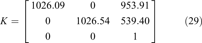
The internal matrix of the camera needs to be calibrated before experiments. The camera calibration algorithm³⁰ is applied with MATLAB, using 20 chessboard images taken from different angles as a calibration template. After calibration, the internal matrix of the camera is

K = [\begin{matrix} 1026.09 & 0 & 953.91 \\ 0 & 1026.54 & 539.40 \\ 0 & 0 & 1 \end{matrix}]

Artificial marker identification experiment

The reliability of the marker recognition has been tested by analyzing the marker detection rate and the marker identification rate. The detection rate indicates the ratio of detected markers to the total number of captured markers. The identification rate means the ratio of correctly identified markers to all the detected markers. In this article, 856 images captured from both the laboratory and the factory environments are tested. There are 1216 markers in these images, and 1188 of them have been detected. In addition, they were all identified successfully. The results are listed in Table 2. Some images were captured in the challenging environment and the makers in them could hardly be detected. So, the misrecognition rate reaches 2.3%. The marker identification rate is 100%, which means information of the finally recognized marker is highly reliable.

Table 2.

The reliability of marker recognition.

Options	Ratio (%)
Marker detection rate	$97.7$
Marker identification rate	$100$
Misrecognition rate	$2.3$

Furthermore, we also analyzed the robustness of the recognition algorithm. We processed the images captured in different illumination conditions. The results are shown in Figure 10. Figure 10(a) shows the normal condition. Figure 10(b) indicates the recognition results under the influence of sunlight, which shone in from the window. Because our system is used in indoor environments, the influence of the sunlight is weak. So, the markers can be recognized easily and accurately in this situation. The influence of the lamp light was also tested in the experiment. We turned on the lamp hanging from the ceiling and moved the robot around to analyze the effect of lamp light. Lamp light has a great impact on the recognition process, but our method can deal with most of the challenging situations. Figure 10(c) shows one sampled image. It can be seen that the marker in it can be recognized correctly. But, when the robot got too close to the lamp, the marker cannot be recognized, as shown in Figure 10(d). So, this factor should be considered when planning the trajectory of the robot. We also processed the images captured in dark environment and our recognition algorithm work well in usual situations, as shown in Figure 10(e). In reality, when it is too dark, the lamp will be turned on, so there is no strict requirement in dark environment. From the experiments, we can learn that the proposed recognized algorithm can work well in most of the challenging illumination conditions.

Figure 10.

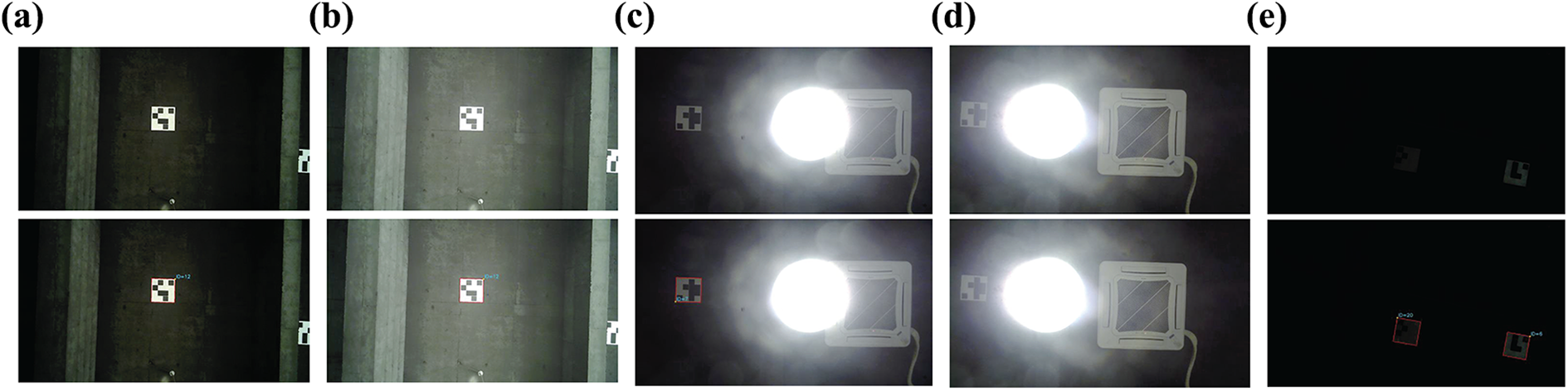
Marker identification in different illumination conditions. (a) normal, (b) sunlight, (c) lamp light, (d) lamp light, and (e) dark.

In addition, we have tested the recognition algorithm in blurred images. Image blurring can be caused by many reasons, of which the most important one is the movement of the mobile robot. When the robot moves at a higher speed, the vibration of the robot will also be more obvious. The high speed and the vibration can cause the image blurring. As shown in Figure 11, the faster the robot moves, the more blurred the images are. However, our markers can be recognized even when the velocity is up to 2.5 m/s, which absolutely meets the application requirements. These evaluation results show the robustness and accuracy of our marker recognition algorithm.

Figure 11.

The marker identification in blurred images of varying degrees. We processed the captured image when the velocity of the mobile robot was (a) 0 m/s, (b) 1 m/s, (c) 2 m/s, and (d) 2.5 m/s.

Marker recognition frequency and the mobile robot’s speed can affect the positioning accuracy. The positioning error caused by the two parameters can be described as $\frac{v_{robot}}{f_{m}}$ , where $v_{robot}$ and f_m indicate the speed of the mobile robot and the marker recognition frequency, respectively. In order to ensure the localization precision, the following condition must be satisfied

f_{m} > \frac{v_{robot}}{d_{error}} or T_{m} < \frac{d_{error}}{v_{robot}}

where $d_{error}$ is the maximum allowable positioning error and T_m indicates the period of marker recognition.

In industry, the maximum speed of the robot may be supposed to be more than 1.5 m/s. The maximum allowable positioning error at this speed should be less than 20 cm. So, T_m should satisfy the following condition

T_{m} < \frac{0.2 m}{1.5 m/s} = 0.13 s

At the end of the trajectory, the localization error may be supposed to be less than 10 cm, and the speed at this situation can be 0.5 m/s. So, T_m should satisfy the following condition

T_{m} < \frac{0.1 m}{0.5 m/s} = 0.2 s

As a result, T_m should be less than 0.13 s. In the experiment, we recorded the marker recognition time of 530 images. The average processing time is 0.016 s per frame, which can totally meet the requirement.

Mapping and positioning experiment

Further experiment has been conducted to test the accuracy of the localization system. In the experiment, we let a robot equipped with an up-facing camera move around on the floor and traverse the working area. After that, the marker map was built using different methods. It was convenient to measure the real position of the robot in this environment. Forty-three actual positions in this place were measured with a ruler whose minimum scale is millimeter. The results of the experiment are shown in Figure 12, of which (a) shows the marker map and (b) indicates the corresponding localization results of 43 sampled positions. The green graph indicates the actual values.

Figure 12.

The experiment results. (a) The marker map in global image coordinate established with different methods. (b) The corresponding positioning results. (c) The time consumption of different methods.

In Figure 12, the black ones are the localization results of the visual odometer method. This method determined the position and orientation of the robot by analyzing the associated two consecutive images. However, it did not consider the loop closure of the map. As a result, this led to a cumulative error in the localization process.

The other two methods took the loop closure detection into account to reduce the accumulated error. The blue drawing shows the performance of the traditional G2O method whose edges included all the obtained relative information between any two nodes. The red ones present the results of our proposed method. It is a kind of improved G2O method which could use the Bayes Estimation method to reduce the edge’s uncertainty when more information is gained. From the figures, we can see that the results of the two graph-based methods both had higher accuracy and were more accurate than the visual odometer method. As shown in Table 3, the average positioning errors of graph-based method are 23.5 mm and 21.4 mm, which is much less than the 69.8 mm of the visual odometer method. Additionally, the graph-based method has also done a better job in orientation performance.

Table 3.

Localization accuracy.

Methods	Visual odometer	Graph-based method
Methods	Visual odometer	Without updating edges	Updating edges
Positioning error (mm)
Average	69.8	23.5	21.4
Maximum	127.0	71.7	68.2
Orientation error (°)
Average	0.38	0.36	0.34
Maximum	1.26	1.09	1.08

As for the two graph-based methods, our proposed method performs better in both accuracy and time efficiency in contrast to the traditional G2O method. In our method, with the uncertainty model, the obtained information with high confidence could contribute more to the edge. However, in the traditional method, every edge, including the one with small confidence, has the same weight. So, our method has a more accurate localization performance, as shown in Figure 12(b) and Table 3 of this article.

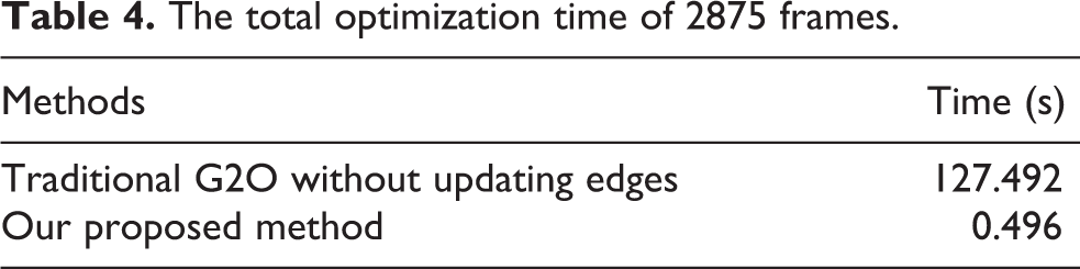
For more accurate localization, the traditional G2O method would consider all the obtained information by adding all the edge information into the graph. That is to say, there exists more than one edge between each two nodes. The more edges in the graph there are, the more time it will take to do the optimization. So, the optimization time of the traditional method will keep increasing when building map. In our method, there exists only one edge between any two nodes, and the edges take all the acquired information into account. When all the nodes are added to the graph, the number of edges is determined and the optimization time of the proposed method will not increase. In the experiment, we captured 2875 frames to test the time-consuming problems of the traditional G2O method and our proposed method. The results are shown in Figure 12(c) and Table 4. When the optimization time of the traditional G2O method reaches 0.1 s per frame, the optimization time of our method is still low, as shown in Figure 12(c). The total optimization time of all 2875 frames of our method is 0.496 s. This is far less than traditional methods’ 127.492 s, as shown in Table 4. So, we can conclude that our proposed method can greatly improve the real-time performance of the robot with less optimization time.

Table 4.

The total optimization time of 2875 frames.

Methods	Time (s)
Traditional G2O without updating edges	127.492
Our proposed method	0.496

From the experiments, we can see that our proposed system not only improves the localization accuracy but also has an improved time-efficiency.

Robustness test in a factory

In this part, our proposed system was used in a forklift, in which the system provided the localization information. The forklift was required to pick up the goods shelf at one specified location and carry it to another. The location error needed to be less than 100 mm and orientation error less than 2°.

In the experiment, we first used our proposed method to build the marker map of the factory. Then, a human driver drove the forklift to perform the transportation work, in which the starting and ending points were accurately measured. During this teaching period, the route was recorded as the planned trajectory by our localization system. Then, the forklift controlled itself along the planned route, and the self-driven trajectory was recorded. The motion curve is shown in Figure 13. The black line indicates the real route edges in the factory. The red line represents the planned route, and the self-driven trajectory is represented by the green line. As shown in Figure 13, there is little variation between the planned trajectory and the self-driven trajectory. From the observation of the movements of the forklift when it is working, we can see that the self-driven trajectory is within reasonable range. From the observations and results of the experiments, it can be concluded that our localization system and the navigation system based on the localization system work very well and can meet the real application requirement. The maximum speed of the forklift could reach 2.5 m/s, which can afford the normal use in industry.

Figure 13.

The motion curve of the forklift.

In contrast to the whole trajectory during the transportation, the localization accuracy in the specified locations, such as the starting and ending points, is required to be higher and more robust. So the transformation was conducted (Figure 14) for 50 times to test its repeated positioning accuracy in the two specified locations. The results are shown in Table 5. During the experiments, our system went very well. From the table, we can see the maximum positioning error is 79.3 mm and the maximum orientation error is 1.36°. So, our system can clearly satisfy the requirements of the industrial environment.

Figure 14.

The process for a forklift to carry goods shelf to specified place. (a) The location where to pick up goods shelf. (b) to (e) The process of carrying goods shelf. (f) The place where the goods shelf should be put on.

Table 5.

Localization accuracy in factory.

positioning error(mm)
Average	25.3
Maximum	79.3
Orientation error (°)
Average	0.14
Maximum	1.36

Conclusion

This article develops an improved artificial marker-based localization system for indoor operation of mobile robots. Firstly, we designed a novel kind of marker which can be detected and identified rapidly and correctly. The markers can be arranged on the ceiling and a robot with an up-facing camera moves around on the floor capturing images. The captured images are processed to get the markers’ information. Secondly, the uncertainty of the camera has been modeled according to the distortion of the camera. The uncertainty of the obtained markers’ information is analyzed through the uncertainty model. Finally, the graph-based optimization algorithm is used to do the loop closure job. In this process, the uncertainty of the edges can be updated through the Bayes Estimation method, as more edge information is obtained. This process can eliminate the accumulated errors, thus improving the localization performance. Results gathered from experimentation have verified that the newly designed marker is robust in different environments and it never recognizes other objects as markers. So the localization system will not make huge mistakes. Additionally, the accuracy of the system was also demonstrated in a laboratory environment, as well as testing its robustness by an industrial application.

In future work, we will analyze the other factors that may have affected the mapping and positioning, such as the image blurring, illumination of the environment, and the uneven ground. Other sensors, such as odometers, can also be used to improve accuracy.

Footnotes

Acknowledgements

The authors would like to thank the National Natural Science Foundation of China and the Hangzhou Civic Significant Technological Innovation Project of China for supporting this work.

Declaration of conflicting interests

The author(s) declared no potential conflicts of interest with respect to the research, authorship, and/or publication of this article.

Funding

The author(s) disclosed receipt of the following financial support for the research, authorship, and/or publication of this article: This work was financially supported by the National Natural Science Foundation of China (grant no: 51521064), the Hangzhou Civic Significant Technological Innovation Project of China (nos: 20131110A04, 20142013A56).

ORCID iD

Yuehua Li

References

Kim

Yoon

. Generating task-oriented interactions of service robots. IEEE Trans Syst Man Cybern 2014; 44(8): 981–994.

Peyraud

Royer

Renault

. Collaborative methods for real-time localization in urban centers. Int J Adv Robot Syst 2015; 12(11): 1–13.

Luo

Lai

. Multisensor fusion-based concurrent environment mapping and moving object detection for intelligent service robotics. IEEE Trans Ind Electron 2014; 61(8): 4043–4051.

Yuan

Song

Zhou

. A novel Mittag-Leffler kernel based hybrid fault diagnosis method for wheeled robot driving system. Comput Int Neurosci 2015; 2015: 606734.1–606734.11.

Reinstein

Hoffmann

. Dead reckoning in a dynamic quadruped robot based on multimodal proprioceptive sensory information. IEEE Trans Robot 2013; 29(2): 563–571.

Luo

Chen

. Wireless and pyroelectric sensory fusion system for indoor human/robot localization and monitoring. IEEE/ASME Trans Mech 2013; 18(3): 845–853.

Müller

Burgard

. Efficient probabilistic localization for autonomous indoor airships using sonar, air flow, and IMU sensors. Adv Robot 2013; 27(9): 711–724.

Hsieh

Tasi

. Visual localization for mobile robots based on composite map. J Robot Mech 2013; 25(1): 25–37.

Song

Xia

Teng

. A precise and real-time loop-closure detection for SLAM using the RSOM Tree. Int J Adv Robot Syst 2015; 12(6): 1–11.

10.

Davison

Reid

Molton

. MonoSLAM: real-time single camera SLAM. IEEE Trans Pattern Anal Mach Intell 2007; 29(6): 1052–1067.

11.

Klein

Murray

. Parallel tracking and mapping for small AR workspaces. In: IEEE and ACM international symposium on mixed and augmented reality. IEEE computer society, Nara, 13–16 November 2007, pp. 1–10, IEEE.

12.

Konolige

Agrawal

. FrameSLAM: from bundle adjustment to real-time visual mapping. IEEE Trans Robot 2008; 24(5): 1066–1077.

13.

Kummerle

Grisetti

Strasdat

. G2O: a general framework for graph optimization. In: International conference on robotics and automation, Shanghai, China, 9–13 May 2011, Vol. 7(8), pp. 3607–3613. IEEE.

14.

Hwang

Song

. Clustering and probabilistic matching of arbitrarily shaped ceiling features for monocular vision-based SLAM. IEEE Trans Adv Robot 2013; 27(10): 739–747.

15.

Choi

Kim

. An efficient ceiling-view slam using relational constraints between landmarks. Int J Adv Robot Syst 2014; 11(1): 4.

16.

Liu

Wang

Chen

. Feature points selection with flocks of features constraint for visual simultaneous localization and mapping. Int J Adv Robot Syst 2016; 14(1): 1–11.

17.

Kabuka

Arenas

. Position verification of a mobile robot using standard pattern. IEEE J Robot Autom 1987; 3(6): 505–516.

18.

Guo

. Landmark design using projective invariant for mobile robot localization. In: Proceedings of the international conference on robotics and biomimetics, Kunming, China, 17–20 December 2007, pp. 852–857. IEEE.

19.

Zhong

Zhou

Liu

. Design and recognition of artificial landmarks for reliable indoor self-localization of mobile robots. Int J Adv Robot Syst 2017; 14(1): 1–13.

20.

Wen

Yuan

Zou

. Visual navigation of an indoor mobile robot based on a novel artificial landmark system. In: International conference on mechatronics and automation, Changchun, China, 9–12 August 2009, pp. 3775–3780. IEEE.

21.

Zheng

Yuan

. MR code for indoor robot self-localization. In: Seventh world congress on intelligent control and automation, Chongqing, China, 25–27 June 2008, pp. 7449–7454. IEEE.

22.

Tian

Duan

. The design of a novel artificial label for robot navigation. In: Proceedings of the Chinese intelligent automation conference, Yangzhou, China, 23–25 August 2013, pp. 479–487. Berlin, Heidelberg: Springer.

23.

Okuyama

Kawasaki

Kroumov

. Localization and position correction for mobile robot using artificial visual landmarks In: International conference on advanced mechatronic systems, Zhengzhou, China, 11–13 August 2011, pp. 414–418. IEEE.

24.

Aleksandrovich

Gennadievich

Stepanovich

. Mobile robot navigation based on artificial landmarks with machine vision system. World Appl Sci J 2013; 24(11): 1467–1472.

25.

Her

Kim

. Localization of mobile robot using laser range finder and IR landmark. In: Proceedings of the 12th international conference on control, automation and systems, JeJu Island, South Korea, 17–21 October 2012, pp. 459–461. IEEE.

26.

Kim

Lee

. An indoor localization system for mobile robots using an active infrared positioning sensor. J Ind Intell Inf 2014; 2(1): 35–38.

27.

Ren

. A method of self-localization of robot based on infrared landmark. In: Proceedings of the 11th world congress on intelligent control and automation, Shenyang, China, 29 June–4 July 2014, pp. 5494–5499. IEEE.

28.

Sultan

Chen

Qadeer

. Vision guided path planning system for vehicles using infrared landmark. In: Proceedings of the IEEE international conference on robotics and biomimetics, Shenzhen, China, 12–14 December 2013, pp. 179–184. IEEE.

29.

Zhou

Yuan

Yang

. A high precision visual localization sensor and its working methodology for an indoor mobile robot. Front Inf Technol Electron Eng 2016; 17: 365.

30.

Zhang

. Flexible camera calibration by viewing a plane from unknown orientations. In: Proceedings of the seventh IEEE International conference on computer vision, Kerkyra, Greece, 20–27 September 1999, pp. 666–673. IEEE.

An improved graph-based visual localization system for indoor mobile robot using newly designed markers

Abstract

Keywords

Introduction

Design and recognition of artificial markers

Design of artificial markers

Extraction and recognition of the marker

The uncertainty model of the camera

Multi-marker-based visual localization system

Parameter determination and coordinates establishment

Graph-based optimization

Localization

Experiments and results

Artificial marker identification experiment

Mapping and positioning experiment

Robustness test in a factory

Conclusion

Footnotes

Acknowledgements

Declaration of conflicting interests

Funding

ORCID iD

References