Sage Journals: Discover world-class research

Abstract

This study presents a new adaptive synchronized computed torque control algorithm based on neural networks for three degree-of-freedom planar parallel manipulators. The basic idea of the proposed control algorithm is to use the incorporation of cross-coupling errors of active joints with the adaptive computed torque control algorithm, online self-tuned neural networks, and error compensators. The key to the success of the proposed approach is to improve the trajectory tracking accuracy of the parallel manipulator’s end-effector while driving the synchronization errors among active joints to zero. The uncertainties of the control system such as modeling errors, frictional terms, and external disturbances are adaptively compensated online during the trajectory tracking of the parallel manipulator. Using the Lyapunov theory, it is proved that the tracking errors and error rates of the overall system asymptotically converge to zero. To demonstrate the effectiveness of the proposed control algorithm, compared simulations are conducted using MATLAB/Simulink [version 2013a] combined with Solidworks 2014.

Keywords

Parallel manipulator synchronized control computed torque control uncertainties compensation neural networks online tuning

Introduction

In the last recent decades, research on the control of parallel manipulators has had drawn a lot of interest in the robotics community. This is because parallel manipulators have potential advantages in terms of high rigidity, high speed, high accuracy, and high load-carrying capacity over serial robotic manipulators. They are widely used in numerous applications such as simulators, humanoid robots, medical robots, micro-robots, and high-accuracy pick-and-place positioning and are becoming increasingly popular in the strict requirements such as small product size and shorter assembly time.

In the literature on tracking control of parallel manipulators, numerous control methods have been proposed, which could be classified as two kinds of approaches. The first one is model-free control approach, such as proportional–derivative (PD) controller,^1,2 nonlinear PD controller,^3,4 and adaptive switching learning PD control method.⁵ The other one is model-based control approach, such as computed torque controllers,^6

–10 the model-based iterative learning controller,¹¹ sliding mode controllers,^12

–16 and the adaptive controllers.^17

–21 The common characteristic of these approaches is that only local feedback information of the controlled joint is fed to the control loop of each individual actuator. Feedback signal from other actuated joints cannot be received. As a result, errors caused by disturbances in the control loop of one actuator are corrected by this loop only, while others do not respond. In parallel manipulators, the trajectory of the end-effector is led by all actuator motions. Therefore, all actuated joints in parallel manipulators should be synchronously controlled to increase the tracking accuracy.

Many works on synchronized control of parallel manipulators have been conducted in recent years. This control approach involves kinematic coupling among the active joints of the parallel manipulators, which results in higher tracking accuracy of the end-effector. The synchronized control approach was first proposed by Koren.²² In his study, the cross-coupling control was used for a multi-axis machining tool to achieve the multi-axis tracking synchronization. It is the employment of the synchronization error that makes the synchronized control different from traditional proportional–integral–derivative control. This useful approach has become more popular in position synchronization control of multiple motion axes,^23,24 mobile robot control,^25,26 and tracking control of parallel manipulators.^27

–32

For tracking control of single parallel manipulators, Sun et al.²⁷ presented a cross-coupled control approach to the tracking control of parallel manipulators in a synchronous manner. On the other hand, Ren et al.²⁸ have proposed a convex synchronized control algorithm for a three degree-of-freedom (3-DOF) planar parallel manipulator. The control algorithm is based on the combination of the advantages of the convex combination method and the synchronized control method. In another approach, a synchronized control algorithm, which does not need dynamic model of parallel manipulators, has been presented such as integration of saturated proportional–integral synchronous control and PD feedback control algorithm.²⁹ In addition, Ren et al.³⁰ presented an adaptive synchronized control method for parallel manipulator based on the combination of synchronized control and adaptive control. Shang et al.³¹ proposed an active joint-synchronization controller to solve control problem of redundantly actuated parallel manipulators. Ren et al.,³² in an experimental comparison study of the synchronized control approaches, have shown that the synchronized control methods based on a dynamic model of the robot can achieve better performance than the model-free ones. However, the model-based synchronized control algorithms are much more complex than the model-free ones due to the complexity of the dynamic model of parallel manipulators. In addition, the aforementioned methods are still complex and require numerous computation to be applied.

In this article, we propose a new synchronized control algorithm for 3-DOF planar parallel manipulators. The control algorithm is based on the combination of synchronization error and cross-coupling error with the computed torque control algorithm and uncertainties compensation method. The uncertainties of the control system such as modeling errors, frictional terms, and external disturbances are adaptively compensated by radial basis function neural networks (RBFNNs) and error compensators. The online weight tuning algorithms of the neural networks and error compensators are derived with the strict theoretical stability proof of the Lyapunov theorem.

The rest of this article is organized as follows. In the second section, the kinematic modeling and dynamic modeling of 3-DOF planar parallel manipulators are formulated in the active joint space. The proposed synchronized computed torque controller (SCTC) is presented in the third section. The comparative simulations are carried out in fourth section in order to verify the effectiveness of the proposed controller. Finally, a conclusion is reached in the fifth section.

Kinematic modeling and dynamic modeling of 3-DOF planar parallel manipulators

The 3-DOF planar parallel robot manipulator is shown in Figure 1. It works on a horizontal plane and in a reference frame Oxy. The manipulator consists of three active joints and six passive joints. The active joints are actuated by actuators, while the passive ones can move freely. The end-effector of the robot is a triangle C ₁ C ₂ C ₃, which connects the ending points of three 2-DOF serial robot manipulators. P is the center point of the end-effector. The 3-DOF planar parallel robot manipulator is controlled by actuating three active joints A ₁, A ₂, and A ₃.

Figure 1.

Three-DOF planar parallel manipulator. DOF: degree of freedom.

We denote the vectors of variable as follows

$q_{a} = {[q_{a 1}, q_{a 2}, q_{a 3}]}^{T}$ is the vector of active joint angulars.

$q_{p} = {[q_{p 1}, q_{p 2}, q_{p 3}]}^{T}$ is the vector of passive joint angulars.

$X = {[x_{P}, y_{P}, ϕ_{P}]}^{T}$ is the vector of Cartesian coordinates and rotate angle of the end-effector.

In the control system, for the 3-DOF planar parallel robot manipulator, the control signal will be sent to drive three active joints of the robot. Therefore, we need to develop kinematic model and dynamic model in active joint space.

Kinematic modeling

Forward kinematics

In the forward kinematics problem, we compute the end-effector’s coordinate $X (x_{p}, y_{p}, ϕ_{p})$ in the reference A ₁ xy from the given active joint angular vector $q_{a} (q_{a 1}, q_{a 2}, q_{a 3})$ .

From Figure 1, we have the following equation system

{[x_{P} - x_{A i} - l_{1} cos q_{a i} - l_{3} cos (ϕ_{P} + ψ_{i})]}^{2} + {[y_{P} - y_{A i} - l_{1} sin q_{a i} - l_{3} sin (ϕ_{P} + ψ_{i})]}^{2} = l_{2}^{2}, i = 1, 2, 3

in which ψ_i (i = 1,2,3) are, respectively, equal to 7π/6, 11π/6, and π/2.

Solving the equation system (1) by applying the numerical method, we obtain coordination x_P , y_P , and the value of ϕ_P with given input qa .

In the control system, we need to know the value of passive joint angles. After having the output X (x_P , y_P ,ϕ_P ), we can compute the value of passive joint angles using the following equation:

q_{p i} = π - {cos}^{- 1} (\frac{l_{1}^{2} + l_{2}^{2} - x_{C i}^{2} - y_{C i}^{2}}{2 l_{1} l_{2}}), i = 1, 2, 3

where the coordinates of the points C_i (i = 1, 2, 3) are computed as follows

x_{C i} = x_{P} + l_{3} cos (ϕ_{P} + ψ_{i}) - x_{A i}, i = 1, 2, 3

y_{C i} = x_{P} + l_{3} sin (ϕ_{P} + ψ_{i}) - y_{A i}, i = 1, 2, 3

Inverse kinematics

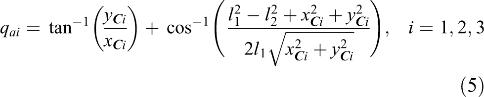
The inverse kinematics problem is to obtain the active joint angular vector $q_{a} (q_{a 1}, q_{a 2}, q_{a 3})$ from the given coordinates $X (x_{P}, y_{P}, ϕ_{P})$ of the end-effector.

From Figure 1, we have the following equations of the inverse kinematics

q_{a i} = {tan}^{- 1} (\frac{y_{C i}}{x_{C i}}) + {cos}^{- 1} (\frac{l_{1}^{2} - l_{2}^{2} + x_{C i}^{2} + y_{C i}^{2}}{2 l_{1} \sqrt{x_{C i}^{2} + y_{C i}^{2}}}), i = 1, 2, 3

Jacobian matrices

We have the following equations obtained from Figure 1

[\begin{matrix} x_{P} \\ y_{P} \end{matrix}] = [\begin{matrix} x_{o i} + l_{1} cos q_{a i} + l_{2} cos (q_{a i} + q_{p i}) \\ y_{o i} + l_{1} sin q_{a i} + l_{2} sin (q_{a i} + q_{p i}) \end{matrix} \begin{matrix} + l_{3} cos (ψ_{i} + ϕ_{P}) \\ + l_{3} sin (ψ_{i} + ϕ_{P}) \end{matrix}], i = 1, 2, 3

By differentiating equation (6) with respect to time, we obtain the following

[\begin{matrix} {\dot{x}}_{P} \\ {\dot{y}}_{P} \end{matrix}] = [\begin{matrix} - l_{1} {\dot{q}}_{a i} sin q_{a i} - l_{2} ({\dot{q}}_{a i} + {\dot{q}}_{p i}) sin (q_{a i} + q_{p i}) \\ l_{1} {\dot{q}}_{a i} cos q_{a i} + l_{2} ({\dot{q}}_{a i} + {\dot{q}}_{p i}) cos (q_{a i} + q_{p i}) \end{matrix} \begin{matrix} - l_{3} {\dot{ϕ}}_{P} sin (ψ_{i} + ϕ_{P}) \\ + l_{3} {\dot{ϕ}}_{P} cos (ψ_{i} + ϕ_{P}) \end{matrix}], i = 1, 2, 3

Rearranging equation (7) leads to an equation under the matrix form

J_{z 1} \dot{X} = J_{o} {\dot{q}}_{a}

where $\dot{X} = {[{\dot{x}}_{P}, {\dot{y}}_{P}, {\dot{ϕ}}_{P}]}^{T}$ corresponds to the velocity of end-effector in the Cartesian coordinate, and ${\dot{q}}_{a} = {[{\dot{q}}_{a 1}, {\dot{q}}_{a 2}, {\dot{q}}_{a 3}]}^{T}$ corresponds to the angular velocity vector of active joints.

Jacobian matrices are expressed by the following equations

J_{z 1} = [\begin{matrix} a z 1_{1} & b z 1_{1} & c z 1_{1} \\ a z 1_{2} & b z 1_{2} & c z 1_{2} \\ a z 1_{3} & b z 1_{3} & c z 1_{3} \end{matrix}]

J_{o} = [\begin{matrix} d z 1_{1} & 0 & 0 \\ 0 & d z 1_{2} & 0 \\ 0 & 0 & d z 1_{3} \end{matrix}]

in which

{\begin{matrix} a z 1_{i} = cos (q_{a i} + q_{p i}) \\ b z 1_{i} = sin (q_{a i} + q_{p i}) \\ c z 1_{i} = - l_{3} sin (q_{a i} + q_{p i} - ψ_{i} - ϕ_{P}) \\ d z 1_{i} = l_{1} sin q_{p i} \end{matrix}; i = 1, 2, 3

Finally, equation (8) could be rewritten as follows

{\dot{q}}_{a} = J_{o z} \dot{X}

where J_oz is the Jacobian matrix

J_{o z} = J_{o}^{- 1} J_{z 1}

Equation (13) could be used for singularity analysis. It could be seen that the singularities of the 3-DOF planar parallel manipulator occur whenever $J_{o}^{- 1}$ , J _z1, or both become singular.

Dynamic modeling

In this section, the dynamic modeling of the 3-DOF planar parallel manipulator is presented in active joint space. For deriving the dynamic model, we follow the method presented by Le and Kang.³³ First, three passive joints C ₁, C ₂, and C ₃ are virtually cut to form an equivalent open-chain system as shown in Figure 2. Second, using the Lagrangian approach, the dynamic model of the equivalent open-chain system can be computed and obtained as follows³⁴

Figure 2.

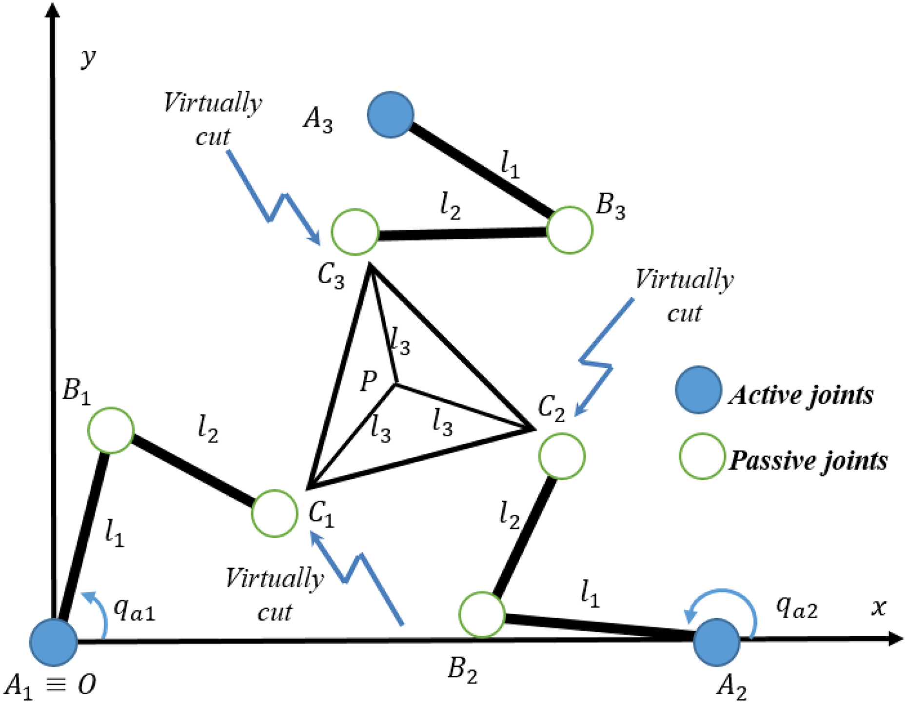
The equivalent open-chain system obtained by virtually cut at C ₁, C ₂, and C ₃.

M_{O} (q) \ddot{q} + C_{O} (q, \dot{q}) \dot{q} + F_{O} = τ_{O}

in which $M_{O} \in ℝ^{9 \times 9}$ is the inertia matrix, $C_{O} \in ℝ^{9 \times 9}$ is the Coriolis and centrifugal force matrix, F _O is the vector of friction forces, $τ_{O} = {[τ_{a}, τ_{p}]}^{T} \in ℝ^{9 \times 1}$ is the joint torque vector of the equivalent open-chain system, $τ_{a} \in ℝ^{3 \times 1}$ is the active joint torque vector, and $τ_{p} \in ℝ^{6 \times 1}$ is the passive joint torque vector. The matrices M _O and C _O are computed by the following equations

M_{O} = [\begin{matrix} δ_{1} & 0 & 0 & ε_{1} & 0 & 0 & 0 & 0 & 0 \\ 0 & δ_{2} & 0 & 0 & ε_{2} & 0 & 0 & 0 & 0 \\ 0 & 0 & δ_{3} & 0 & 0 & ε_{3} & 0 & 0 & 0 \\ η_{1} & 0 & 0 & β_{1} & 0 & 0 & 0 & 0 & 0 \\ 0 & η_{2} & 0 & 0 & β_{2} & 0 & 0 & 0 & 0 \\ 0 & 0 & η_{3} & 0 & 0 & β_{3} & 0 & 0 & 0 \\ 0 & 0 & 0 & 0 & 0 & 0 & m_{P} & 0 & 0 \\ 0 & 0 & 0 & 0 & 0 & 0 & 0 & m_{P} & 0 \\ 0 & 0 & 0 & 0 & 0 & 0 & 0 & 0 & I_{P} \end{matrix}]

C_{O} = [\begin{matrix} ϑ_{1} & 0 & 0 & μ_{1} & 0 & 0 & 0 & 0 & 0 \\ 0 & ϑ_{2} & 0 & 0 & μ_{2} & 0 & 0 & 0 & 0 \\ 0 & 0 & ϑ_{3} & 0 & 0 & μ_{3} & 0 & 0 & 0 \\ ρ_{1} & 0 & 0 & 0 & 0 & 0 & 0 & 0 & 0 \\ 0 & ρ_{2} & 0 & 0 & 0 & 0 & 0 & 0 & 0 \\ 0 & 0 & ρ_{3} & 0 & 0 & 0 & 0 & 0 & 0 \\ 0 & 0 & 0 & 0 & 0 & 0 & 0 & 0 & 0 \\ 0 & 0 & 0 & 0 & 0 & 0 & 0 & 0 & 0 \\ 0 & 0 & 0 & 0 & 0 & 0 & 0 & 0 & 0 \end{matrix}]

F_{O} = {[f_{a 1}, f_{a 2}, f_{a 3}, f_{b 1}, f_{b 2}, f_{b 3}, f_{c 1}, f_{c 2}, f_{c 3}]}^{T}

where $δ_{i} = α_{i} + β_{i} + 2 γ_{i} cos q_{p i}$ , $ε_{i} = β_{i} + γ_{i} cos q_{p i}$ , $ϑ_{i} = - 2 γ_{i} {\dot{q}}_{p i} sin q_{p i}$ , $η_{i} = β_{i} + γ_{i} cos q_{p i}$ , $α_{i} = m_{i 1} l_{c 1}^{2} + m_{i 1} l_{2}^{2} + I_{i 1}$ , $β_{i} = m_{i 2} l_{c 2}^{2} + I_{i 2}$ , $γ_{i} = m_{i 2} l_{c 1} l_{c 2}$ , and f_ai , f_bi , and f_ci are the friction forces at joints of the robot $(i = 1, 2, 3)$ .

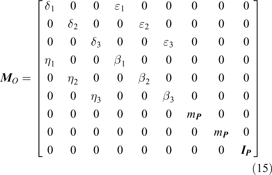
Since the parallel manipulator is controlled by actuating three active joints A ₁, A ₂, and A ₃, we need to develop the dynamic model in the active joint space with the input torque $τ_{a} = {(τ_{a 1}, τ_{a 2}, τ_{a 3})}^{T} \in ℝ^{3 \times 1}$ . Following the D’Alembert principle and principle of virtual work, we have the following relationship³⁵

W^{T} τ_{O} = τ_{a}

where W is the Jacobian matrix

W = [\begin{matrix} I \\ \frac{\partial q_{p}}{\partial q_{a}} \\ \frac{\partial X_{p}}{\partial q_{a}} \end{matrix}] = [\begin{matrix} I \\ J_{1} \\ J_{2} \end{matrix}] = [\begin{matrix} I \\ J_{o z}^{- 1} J_{p z} \\ J_{o z}^{- 1} \end{matrix}]

where $I \in ℝ^{3 \times 3}$ is the identity matrix. The matrices J_pz is computed as follows

J_{p z} = J_{p}^{- 1} J_{z 2}

where

J_{p} = [\begin{matrix} d z 2_{1} & 0 & 0 \\ 0 & d z 2_{2} & 0 \\ 0 & 0 & d z 2_{3} \end{matrix}]

J_{z 2} = [\begin{matrix} a z 2_{1} & b z 2_{1} & c z 2_{1} \\ a z 2_{2} & b z 2_{2} & c z 2_{2} \\ a z 2_{3} & b z 2_{3} & c z 2_{3} \end{matrix}]

{\begin{matrix} a z 2_{i} = l_{1} cos q_{a i} + l_{c 2} cos (q_{a i} + q_{p i}) \\ b z 2_{i} = l_{1} sin q_{a i} + l_{c 2} sin (q_{a i} + q_{p i}) \\ c z 2_{i} = l_{2} l_{3} sin (ψ_{i} + ϕ_{P} - q_{a i} - q_{p i}) + l_{1} l_{3} sin (ψ_{i} + ϕ_{P} - q_{a i}) \\ d z 2_{i} = - l_{c 1} l_{c 2} sin q_{p i} \end{matrix}, i = 1, 2, 3

By multiplying both sides of equation (14) by W^T and using the relationship in equation (15), we obtain the following

W^{T} (M_{O} (q) \ddot{q} + C_{O} (q, \dot{q}) \dot{q} + F_{O}) = τ_{a}

In addition, we have the following relationships

\dot{q} = {[I, \partial q_{p} / \partial q_{a}, \partial X_{P} / \partial q_{a}]}^{T} {\dot{q}}_{a} = W {\dot{q}}_{a}

\ddot{q} = \dot{W} {\dot{q}}_{a} + W {\ddot{q}}_{a}

By substituting equations (25) and (26) into equation (24) and rearranging the new equation, we obtain the following

{\hat{M}}_{a} {\ddot{q}}_{a} + {\hat{C}}_{a} {\dot{q}}_{a} + F_{a} = τ_{a}

where ${\hat{M}}_{a} = W^{T} M_{O} W \in ℝ^{3 \times 3}$ is the estimated inertia matrix, ${\hat{C}}_{a} = W^{T} M_{O} \dot{W} + W^{T} C_{O} W \in ℝ^{3 \times 3}$ is the estimated Coriolis and centrifugal force matrix, and $F_{a} = W^{T} F_{O} \in ℝ^{3 \times 1}$ is the vector of friction torques in active joints.

The dynamic model in equation (27) satisfies the following properties, which were proved by Cheng et al.³⁶

${\hat{M}}_{a}$ is a symmetric and positive definite matrix.

${\dot{\hat{M}}}_{a} - 2 {\hat{C}}_{a}$ is a skew-symmetric matrix.

In the presence of bounded uncertainties such as errors of dynamic model and external disturbances, we can express the actual dynamic model of the parallel manipulator by the following equation

M_{a} {\ddot{q}}_{a} + C_{a} {\dot{q}}_{a} + F_{a} + d_{a} = τ_{a}

where $M_{a} = {\hat{M}}_{a} + Δ M_{a}$ and $C_{a} = {\hat{C}}_{a} + Δ C_{a}$ are the actual dynamic parameters, d _a is the vector of external disturbances on active joints, and Δ M _a and Δ C _a are dynamic modeling errors.

Finally, we obtain the actual dynamic equation of the 3-DOF planar parallel manipulator as follows

{\hat{M}}_{a} {\ddot{q}}_{a} + {\hat{C}}_{a} {\dot{q}}_{a} + Δ τ_{a} = τ_{a}

in which Δ τ _a is the vector of modeling errors, friction forces, and external disturbances

Δ τ_{a} = Δ M_{a} {\ddot{q}}_{a} + Δ C_{a} {\dot{q}}_{a} + F_{a} + d_{a}

Proposed adaptive SCTC

Define the tracking error

e = q_{d a} (t) - q_{a} (t)

in which $q_{d a} (t) \in ℝ^{3 \times 1}$ is the desired trajectory of the active joint angles.

In the synchronized control methods, not only the tracking error of each individual active joint must come to zero (e_ai (t) → 0, i = 1, 2, 3) but also the tracking errors of all active joints must be equal during the trajectory tracking control

e_{a 1} (t) = e_{a 2} (t) = e_{a 3} (t)

The synchronization errors are defined as follows

E_{1} (t) = e_{a 1} (t) - e_{a 2} (t)

E_{2} (t) = e_{a 2} (t) - e_{a 3} (t)

E_{3} (t) = e_{a 3} (t) - e_{a 1} (t)

The vector of synchronization error is $E = {[E_{1} (t), E_{2} (t), E_{3} (t)]}^{T}$ . Under the synchronization error definition, control torques τ _ai are to control position errors e_ai(t) → 0 and, at the same time, to synchronize the motions of active joints (i = 1, 2, 3).

To accommodate both position error and synchronization error, cross-coupling error insight has been introduced to provide an effective method to eliminate the interconnections among multiple motion axes systems. The cross-coupling error is defined by the following

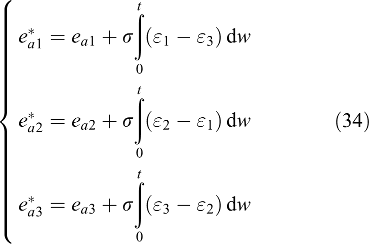
{\begin{matrix} e_{a 1}^{*} = e_{a 1} + σ \int_{0}^{t} (ε_{1} - ε_{3}) d w \\ e_{a 2}^{*} = e_{a 2} + σ \int_{0}^{t} (ε_{2} - ε_{1}) d w \\ e_{a 3}^{*} = e_{a 3} + σ \int_{0}^{t} (ε_{3} - ε_{2}) d w \end{matrix}

in which σ is the positive parameter and w is the time variable.

The reference tracking velocity and the reference tracking acceleration are defined as follows

{\dot{q}}_{d a}^{r} = {\dot{q}}_{d a} + σ Δ ε

{\ddot{q}}_{d a}^{r} = {\ddot{q}}_{d a} + σ Δ \dot{ε}

in which $Δ ε = {[ε_{1} - ε_{3}, ε_{2} - ε_{1}, ε_{3} - ε_{2}]}^{T}$ and $Δ \dot{ε} = {[{\dot{ε}}_{1} - {\dot{ε}}_{3}, {\dot{ε}}_{2} - {\dot{ε}}_{1}, {\dot{ε}}_{3} - {\dot{ε}}_{2}]}^{T}$ .

The proposed controller is expressed by the following equation

τ_{a} = {\hat{M}}_{a} ({\ddot{q}}_{d a}^{r} + K_{v} {\dot{e}}_{a}^{*} + K_{p} e_{a}^{*}) + {\hat{C}}_{a} {\dot{q}}_{a} + τ_{cp} + τ_{er}

where $e_{a}^{*} = {[e_{a 1}^{*}, e_{a 2}^{*}, e_{a 3}^{*}]}^{T}$ is the vector of cross-coupling errors, $K_{v} = diag {k_{v 1}, k_{v 2}, k_{v 3}}$ and $K_{p} = diag {k_{p 1}, k_{p 2}, k_{p 3}}$ are the positive constant parameter matrices, and $τ_{cp} \in ℜ^{3 \times 1}$ is the uncertainty compensation controller which contains a bank of neural network inside for estimating vector ▵ τ _a . Since the term τ _cp cannot perfectly estimate ▵ τ _a , the term τ _er is added to compensate the error of the estimation. The block diagram of the proposed controller is shown in Figure 3.

Figure 3.

Flow diagram of the proposed synchronized computed torque controller.

The proposed controller has some major contributions. First, the combination of synchronization error and cross-coupling error with computed torque control algorithm brings about the advantages of the two methods such as the high accuracy and low online computational burden. The second contribution is the error estimators with online adaptation law, which helps to compensate the estimation errors of the neural network.

From equations (37) and (30), we obtain the following

{\ddot{e}}_{a}^{*} + K_{v} {\dot{e}}_{a}^{*} + K_{p} e_{a}^{*} = {\hat{M}}_{a}^{- 1} (Δ τ_{a} - τ_{cp} - τ_{er})

We define

ρ = {\hat{M}}_{a}^{- 1} Δ τ_{a}

and then the compensative control law τ _cp is defined as follows

τ_{cp} = {\hat{M}}_{a} \hat{ρ}

in which $\hat{ρ}$ is the vector of a bank of RBFNNs for online approximation of Δ τ _a. The structure of each RBFNN used in this study is shown in Figure 4. It is a fixed three-layer network whose output is determined by specified hidden units in certain local receptive fields.^37
–39

Figure 4.

Structure of an RBFNN with L hidden units. RBFNN: radial basis function neural network.

The basis functions in the hidden layer are chosen as Gaussian function and can be expressed as follows

R_{i j} (x_{i}) = exp (- \frac{∥ x_{i} - c_{i j} ∥^{2}}{2 m_{i j}^{2}}), j = 1, 2, \dots, L; i = 1, 2, 3

where x is an N-dimensional input vector, c _ij is a center vector with the same dimension as x , m_ij is the variance of the basic function, L is the number of hidden units in the hidden layer, and ‖.‖ denotes the Euclidean norm.

The output of the RBFNN is computed by the weighted sum method^40,41

{\hat{ρ}}_{i} = \sum_{j = 1}^{L} {\hat{w}}_{i j} R_{i j} (x_{i}) = {\hat{W}}_{i}^{T} R_{i} (x_{i})

{\hat{W}}_{i} = {[{\hat{w}}_{i 1}, {\hat{w}}_{i 2}, \dots, {\hat{w}}_{i L}]}^{T}, i = 1, 2, 3

R_{i} (x_{i}) = {[R_{i 1} (x_{i}), R_{i 2} (x_{i}), \dots, R_{i L} (x_{i})]}^{T}, i = 1, 2, 3

The input vector x _i of each RBFNN is used as follows

x_{i} = {[e_{a i}^{*}, {\dot{e}}_{a i}^{*}]}^{T}, i = 1, 2, 3

where $e_{a i}^{*}$ and ${\dot{e}}_{a i}^{*}$ are, respectively, the tracking cross-coupling error and derivative of cross-coupling error of each active joint of the parallel manipulator.

Then, the vector $\hat{ρ} \in ℜ^{3}$ can be written as follows

\hat{ρ} = [\begin{matrix} {\hat{ρ}}_{1} \\ {\hat{ρ}}_{2} \\ {\hat{ρ}}_{3} \end{matrix}] = [\begin{matrix} {\hat{W}}_{1}^{T} R_{1} (x_{1}) \\ {\hat{W}}_{2}^{T} R_{2} (x_{2}) \\ {\hat{W}}_{3}^{T} R_{3} (x_{3}) \end{matrix}]

It has been shown that for some sufficiently large number of hidden layer neurons, there are ideal weights and thresholds such that ρ can be represented by the following

ρ = [\begin{matrix} W_{1}^{* T} R_{1} (x_{1}) \\ W_{2}^{* T} R_{2} (x_{2}) \\ W_{3}^{* T} R_{3} (x_{3}) \end{matrix}] + [\begin{matrix} ϑ_{1} \\ ϑ_{2} \\ ϑ_{3} \end{matrix}]

where W _i* is the bounded ideal weight vector of the output layer, and ϑ _i is the bounded error (i = 1, 2, 3).

Theorem

Consider the dynamic model in equation (29) of the 3-DOF planar parallel manipulator together with the proposed controller in equation (37). If we choose the following adaptation tuning laws for the RBFNN and the error estimators

${\dot{\hat{W}}}_{i} = μ_{i} X_{i}^{T} P_{i} B_{i} R_{i} (x_{i})$
48

${\dot{\hat{ϑ}}}_{i} = η_{i} X_{i}^{T} P_{i} B_{i}$
49

then the closed-loop system is asymptotically stable.

Proof

By substituting equations (46), (47), (40), and (39) into equation (38), we obtain the following

${\ddot{e}}_{a}^{} + K_{v} {\dot{e}}_{a}^{} + K_{p} e_{a}^{} = [\begin{matrix} {\tilde{W}}_{1}^{T} R_{1} (x_{1}) \\ {\tilde{W}}_{2}^{T} R_{2} (x_{2}) \\ {\tilde{W}}_{3}^{T} R_{3} (x_{3}) \end{matrix}] + ϑ - {\hat{M}}_{a}^{- 1} τ_{e r}$
50

where ${\tilde{W}}_{i} = W_{i}^{} - \hat{W}$ is the weight estimation error and $ϑ = {[ϑ_{1}, ϑ_{2}, ϑ_{3}]}^{T}$ is the vector of errors.

Next, we define the error estimator as follows

$τ_{er} = {\hat{M}}_{a} \hat{ϑ}$
51

where $\hat{ϑ}$ is the estimated value of ϑ .

Now, by substituting equation (51) into equation (50), we obtain the following

${\ddot{e}}_{a}^{} + K_{v} {\dot{e}}_{a}^{} + K_{p} e_{a}^{} = [\begin{matrix} {\tilde{W}}_{1}^{T} R_{1} (x_{1}) \\ {\tilde{W}}_{2}^{T} R_{2} (x_{2}) \\ {\tilde{W}}_{3}^{T} R_{3} (x_{3}) \end{matrix}] + \tilde{ϑ}$
52

where $\tilde{ϑ} = ϑ - \hat{ϑ}$ .

Equation (52) is equivalent to the following equation

${\begin{matrix} {\ddot{e}}_{a 1}^{} + k_{v 1} {\dot{e}}_{a 1}^{} + k_{p 1} e_{a 1}^{} = {\tilde{W}}_{1}^{T} R_{1} (x_{1}) + {\tilde{ϑ}}_{1} \\ {\ddot{e}}_{a 2}^{} + k_{v 2} {\dot{e}}_{a 2}^{} + k_{p 2} e_{a 2}^{} = {\tilde{W}}_{2}^{T} R_{2} (x_{2}) + {\tilde{ϑ}}_{2} \\ {\ddot{e}}_{a 3}^{} + k_{v 3} {\dot{e}}_{a 3}^{} + k_{p 3} e_{a 3}^{} = {\tilde{W}}_{3}^{T} R_{3} (x_{3}) + {\tilde{ϑ}}_{3} \end{matrix}$
53

For each active joint, supposed that state vector is defined as $X_{i} = {[e_{a i}^{}, {\dot{e}}_{a i}^{}]}^{T}, i = 1, 2, 3$ , we obtain the following state equations

${\dot{X}}_{i} = A_{i} X_{i} + B_{i} ({\tilde{W}}_{i}^{T} R_{i} (x_{i}) + {\tilde{ϑ}}_{i}), i = 1, 2, 3$
54

in which

$A_{i} = [\begin{matrix} 0 & 1 \\ - k_{p i} & - k_{v i} \end{matrix}]; B_{i} = [\begin{matrix} 0 \\ 1 \end{matrix}]$

Then, the Lyapunov equation for each active joint can be formulated as follows

$A_{i}^{T} P_{i} + P_{i} A_{i} = - Q_{i}$
55

where P _i and Q _i are positive definite matrices (i = 1, 2, 3). We can choose a positive definite matrix Q _i , and then the positive definite matrix P _i is solved from the Lyapunov equation (55).

For analyzing the stability of the control system, a positive definite Lyapunov function candidate is chosen as follows

$V = \sum_{i = 1}^{3} X_{i}^{T} P_{i} X_{i} + \frac{1}{2} \sum_{i = 1}^{3} μ_{i}^{- 1} {\tilde{W}}_{i}^{T} {\tilde{W}}_{i} + \frac{1}{2} \sum_{i = 1}^{3} η_{i}^{- 1} {\tilde{ϑ}}_{i}^{2}$
56

where ${\tilde{ϑ}}_{i} = ϑ_{i} - {\hat{ϑ}}_{i}$ , and μ_i and η_i are the learning rates with positive values (i = 1, 2, 3).

Differentiating V respect to time, we get the following

$\dot{V} = \sum_{i = 1}^{3} ({\dot{X}}_{i}^{T} P_{i} X_{i} + X_{i}^{T} P_{i} {\dot{X}}_{i}) - \sum_{i = 1}^{3} μ_{i}^{- 1} {\tilde{W}}_{i}^{T} {\dot{\hat{W}}}_{i} - \sum_{i = 1}^{3} η_{i}^{- 1} {\tilde{ϑ}}_{i} {\dot{\hat{ϑ}}}_{i}$
57

By substituting equations (53) and (55) into equation (57), we obtain the following

$\dot{V} = - \sum_{i = 1}^{3} X_{i}^{T} Q_{i} X_{i} + \sum_{i = 1}^{3} X_{i}^{T} P_{i} B_{i} {\tilde{W}}_{i}^{T} R_{i} (x_{i}) + \sum_{i = 1}^{3} X_{i}^{T} P_{i} B_{i} {\tilde{ϑ}}_{i} - \sum_{i = 1}^{3} μ_{i}^{- 1} {\tilde{W}}_{i}^{T} {\dot{\hat{W}}}_{i} - \sum_{i = 1}^{3} η_{i}^{- 1} {\tilde{ϑ}}_{i} {\dot{\hat{ϑ}}}_{i}$
58

Now, by replacing the adaptation tuning laws in equations (48) and (49) into equation (58), we obtain the following

$\dot{V} = - \sum_{i = 1}^{3} X_{i}^{T} Q_{i} X_{i} \leq 0$
59

Since Q_i is a positive definite matrix, $\dot{V} = 0$ only when X _i = 0, i = 1, 2, 3. Therefore, we can see that the control system is asymptotically stable with respect to X _i . It means that

$lim_{t \to \infty} X_{i} = 0, i = 1, 2, 3$

Or equivalent to (i = 1,2,3)

${\begin{matrix} lim_{t \to \infty} e_{i} = 0 = > lim_{t \to \infty} q_{a i} = q_{d a i} \\ lim_{t \to \infty} {\dot{e}}_{i} = 0 = > lim_{t \to \infty} {\dot{q}}_{a i} = {\dot{q}}_{d a i} \end{matrix}$

Thus, it is proved that, with the proposed controller, the actual active joint positions converge to their desired values.

Simulation

To illustrate the effectiveness of the proposed controller in this article, the simulations are performed for a 3-DOF planar parallel manipulator. Simulations are conducted by using the combination of Solidworks 2014 and SimMechanics of MATLAB [version 2013a]. First, the 3-D computer-aided design (CAD) model of the parallel manipulator is built in Solidworks. Each mechanical part of the parallel manipulator is designed separately and assembled using the suitable joints. Second, the 3-D CAD model is exported to an XML file by using the SimMechanics link plug-in. This link plug-in is downloaded from Mathworks official website. The XML file is then imported into Simulink environment. By this way, the geometry from the CAD assembly is saved as geometry files and associated with the proper body in SimMechanics. In the next step, joint actuators, sensors, and friction forces are added to the mechanical model. This mechanical model is then connected to the control algorithm block, which is written in Simulink.

In Solidworks, there is a special tool to verify the dynamic parameters of each component and the whole manipulator platform. The dynamic parameters are presented in Table 1.

Table 1.
Parameters of the parallel manipulator.

Variable Description Value Unit

l ₁ Length of the lower part of each leg 0.4 m

l ₂ Length of the upper part of each leg 0.6 m

l ₃ Dimension of the moving platform 0.2 m

l _c1 Distance from the joint to the mass center of the lower part of each leg 0.2 m

l _c2 Distance from the joint to the mass center of the upper part of each leg 0.3 m

m _i1 Mass of the the lower part of each leg 5.12 kg

m _i2 Mass of the upper part of each leg 7.39 kg

m _p Mass of the moving platform 3.84 kg

I _i1 Moment of inertia of the lower of ith leg 91 × 10⁻³ kg·m²

I _i2 Moment of inertia of the upper of ith leg 267 × 10⁻³ kg·m²

I _p Moment of inertia of the moving platform 65 × 10⁻³ kg·m²

To evaluate the effectiveness of the proposed adaptive SCTC, the following control algorithms for the 3-DOF planar parallel manipulator are simulated and compared:
1. The traditional computed torque controller for parallel manipulator was presented by Le et al.¹⁰
$τ_{a} = {\hat{M}}_{a} ({\ddot{q}}_{d a} + K_{v} {\dot{e}}_{a} + K_{p} e_{a}) + {\hat{C}}_{a} {\dot{q}}_{a}$
60

where K _v and K _p are chosen as $K_{v} = diag {25, 25, 25}$ and $K_{p} = diag {50, 50, 50}$ .

2. The SCTC without uncertainties and external disturbances compensation
$τ_{a} = {\hat{M}}_{a} ({\ddot{q}}_{d a}^{r} + K_{v} {\dot{e}}_{a}^{} + K_{p} e_{a}^{}) + {\hat{C}}_{a} {\dot{q}}_{a}$
61

in which K _v and K _p are also chosen as $K_{v} = diag {25, 25, 25}$ and $K_{p} = diag {50, 50, 50}$ .

3. The proposed control algorithm is described by equation (37). The matrices K _v and K _p have the same value to cases 1 and 2. Other parameters are chosen as σ = 0.1, the number of neuron in the hidden layer L = 25, and the center vector of each basis function neural network is $c_{j k} = {[- 0.5, - 0.25, 0, 0.25, 0.5]}^{T}$ (j = 1, 2, 3, 4, 5; k = 1, 2, 3, 4, 5). These values of parameters are obtained by trial and error method.

The desired trajectory of the end-effector of the 3-DOF planar parallel manipulator is

${\begin{matrix} x = 0.49 + 0.03 cos (\frac{π t}{3}) \\ y = 0.37 + 0.03 sin (\frac{π t}{3}) \\ ϕ = π / 2 \end{matrix}$
62

Friction forces at each active joint of the parallel manipulator are included as follows

$F_{a i} = 0.5 sign ({\dot{q}}_{a i}) + 0.4 {\dot{q}}_{a i} i = 1, 2, 3$
63

The results of tracking trajectory are shown in Figure 5. The end-effector is controlled to track a circular in 20 s. The initial point of the end-effector of the manipulator is A ₀(0.528,0.368). From Figure 5, we can see that the tracking trajectory caused by the conventional computed torque control algorithm has the biggest difference from the reference trajectory. The synchronized computed torque control algorithm (without uncertainties compensation) and the proposed adaptive SCTC produce better results than the conventional CTC. When focusing on the starting point A ₀, it can be seen that the proposed SCTC has the fastest convergence speed to the reference trajectory among the three controllers.

Figure 5.
Results of tracking circular trajectory of conventional CTC (green line), SCTC (blue line), and the proposed ASCTC (red line). CTC: computed torque controller; SCTC: synchronized computed torque controller.

Figure 6 shows the tracking errors of active joints 1, 2, and 3 of the parallel manipulator in active joint space. It is observed that the errors caused by the SCTC are much smaller than the errors associated with the conventional CTC. Especially the proposed adaptive synchronized computed torque controller (ASCTC) brings about the smallest tracking errors compared with the SCTC without uncertainty compensation and the conventional CTC. Additionally, it can be seen that the errors caused by the proposed ASCTC are very small, almost equal to zero.

Figure 6.
Comparison of tracking errors in active joint space: (a) error of active joint 1, (b) error of active joint 2, and (c) error of active joint 3.

The tracking errors of the end-effector in the X-direction, in the Y-direction, and the error of rotary angle are shown in Figure 7. As can be seen from the figure, the SCTC produces smaller tracking errors compared to the conventional CTC. Interestingly, among the three controllers, the proposed ASCTC has the smallest tracking errors. Hence, we can conclude that the proposed ASCTC is highly efficient in control of a 3-DOF planar parallel manipulator. Additionally, it is concluded that the model uncertainties and external disturbances could be greatly tolerated using the proposed ASCTC.

Figure 7.
Comparison of tracking errors of the end-effector: (a) error in the X-direction, (b) error in the Y-direction, and (c) error of rotary angle.

The weight tuning histories of the radial basis function network in each active joint are shown in Figure 8(a). The initial output weight matrices are W _i (0) = 0.01 × I . It can be observed that the weights remain bounded. Figure 8(b) shows the results of online tuning, the output of error compensators. The learning rate matrices are μ_i = 0.0015 and η_i = 0.01 (i = 1, 2, 3). The results showed that the outputs of error compensators are also bounded.

Figure 8.
(a) The weight tuning histories of the radial basis function networks and (b) the results of online tuning, the output of error compensators.

From the simulations, we found that the major obstacle in the development of the control system with the proposed controller is the parameters of the RBFNN such as the centers and variances. It is quite difficult to choose the suitable values for these parameters. In future works, we are going to overcome this difficulty by applying the fully online tuning method for RBFNN, which was proposed by Le and Kang.³³

Conclusion

An adaptive synchronized computed torque control algorithm based on neural networks and error compensators has been proposed in this article. By integrating the definitions of synchronization error, and cross-coupling error of active joints with an adaptive computed torque control algorithm, the results inherit the advantages of both methods, such as the high accuracy and low online computational burden. The proposed control algorithm handles the uncertainties and external disturbances using a bank of neural networks and error compensators. The weights of neural networks and error compensators are adaptively tuned online during the tracking trajectory of the parallel manipulator. The stability of the closed-loop control system is theoretically proved by the Lyapunov method. The results of computer simulations verified the effectiveness of the proposed control algorithm. In the future research direction, a real implementation on the experimental system will be conducted.

Variable	Description	Value	Unit
l ₁	Length of the lower part of each leg	0.4	m
l ₂	Length of the upper part of each leg	0.6	m
l ₃	Dimension of the moving platform	0.2	m
l _c1	Distance from the joint to the mass center of the lower part of each leg	0.2	m
l _c2	Distance from the joint to the mass center of the upper part of each leg	0.3	m
m _i1	Mass of the the lower part of each leg	5.12	kg
m _i2	Mass of the upper part of each leg	7.39	kg
m _p	Mass of the moving platform	3.84	kg
I _i1	Moment of inertia of the lower of ith leg	91 × 10⁻³	kg·m²
I _i2	Moment of inertia of the upper of ith leg	267 × 10⁻³	kg·m²
I _p	Moment of inertia of the moving platform	65 × 10⁻³	kg·m²

Footnotes

Declaration of conflicting interests

The author(s) declared no potential conflicts of interest with respect to the research, authorship, and/or publication of this article.

Funding

The author(s) disclosed receipt of the following financial support for the research, authorship, and/or publication of this article: This research is funded by the Ministry of Education and Training (MOET) of the Socialist Republic of Vietnam, under grant number KYTH-17.

References

Ghorbel

Chetelat

Gunawardana

. Modeling and set point control of closed-chain mechanisms: theory and experiment. IEEE Trans Control Syst Technol 2000; 8: 801–815.

Yang

Huang

Jiang

. PD control with gravity compensation for hydraulic 6-DOF parallel manipulator. Mech Mach Theor 2010; 45: 666–677.

Ouyang

Zhang

. Nonlinear PD control for trajectory tracking with consideration of the design for control methodology. In: Proceedings. ICRA’02. IEEE international conference on robotics and automation, Washington, DC, USA, 11–15 May 2002, Vol. 4, pp. 4126–4131. IEEE.

Dong

. Nonlinear PD synchronized control for parallel manipulators. In: ICRA. Proceedings of the 2005 IEEE international conference on robotics and automation, Barcelona, Spain, 18–22 April 2005, pp. 1374–1379. IEEE.

Ouyang

Zhang

Gupta

. An adaptive switching learning control method for trajectory tracking of robot manipulators. Mechatronics 2006; 16: 51–61.

Yang

Mei

. Motor-mechanism dynamic model based neural network optimized computed torque control of a high speed parallel manipulator. Mechatronics 2007; 17: 381–390.

Paccot

Lemoine

Andreff

. A vision-based computed torque control for parallel kinematic machines. In: ICRA. IEEE international conference on robotics and automation, Pasadena, CA, USA, 19–23 May 2008, pp. 1556–1561. IEEE.

Shang

Cong

. Nonlinear computed torque control for a high-speed planar parallel manipulator. Mechatronics 2009; 19: 987–992.

Yang

Mei

. Mechatronic model based computed torque control of a parallel manipulator. Int J Adv Robotic Syst 2008; 5(1): 123–128.

10.

Kang

Suh

. An online self-gain tuning method using neural networks for nonlinear PD computed torque controller of a 2-dof parallel manipulator. Neurocomputing 2012; 116: 53–61.

11.

Abdellatif

Heimann

. Advanced model-based control of a 6-DOF hexapod robot: a case study. IEEE/ASME Trans Mech 2010; 15: 269–279.

12.

Kim

Cho

Lee

KII

. Robust nonlinear task space control for 6 DOF parallel manipulator. Automatica 2005; 41(9): 1591–1600.

13.

Guo

Liu

. Cascade control of a hydraulically driven 6-DOF parallel robot manipulator based on a sliding mode. Control Eng Pract 2008; 16: 1055–1068.

14.

Begon

Pierrot

Dauchez

. Fuzzy sliding mode control of a fast parallel robot: Proceedings., IEEE international conference on robotics and automation, Nagoya, Japan, 21–27 May 1995, Vol. 1, pp. 1178–1183. IEEE.

15.

Kang

Suh

. Chattering-free neuro-sliding mode control of 2-DOF planar parallel manipulators. Int J Adv Robotic Syst 2013; 10(1): 22.

16.

McInroy

Jafari

. Trajectory tracking with parallel robots using low chattering, fuzzy sliding mode controller. J Int Robotic Syst 2007; 48: 333–356.

17.

Ryu

Song

Kwon

. A nonlinear friction compensation method using adaptive control and its practical application to an in-parallel actuated 6-DOF manipulator. Control Eng Pract 2001; 9: 159–167.

18.

Zhu

Tao

Yao

. Adaptive robust posture control of parallel manipulator driven by pneumatic muscles with redundancy. IEEE/ASME Trans Mech 2008; 13: 441–450.

19.

Zhu

Tao

Yao

. Adaptive robust posture control of a parallel manipulator driven by pneumatic muscles. Automatica 2008; 44: 2248–2257.

20.

Honegger

Brega

Schweiter

. Application of a nonlinear adaptive controller to a 6 DOF parallel manipulator. In: Proceedings. ICRA. IEEE international conference on robotics and automation, San Francisco, CA, USA, 24–28 April 2000, Vol. 2, pp. 1930–1935. IEEE.

21.

Zhu

Tao

Yao

. Integrated direct/indirect adaptive robust posture trajectory tracking control of a parallel manipulator driven by pneumatic muscles. IEEE Trans Control Syst Technol 2009; 17: 576–588.

22.

Koren

. Cross-coupled biaxial computer control for manufacturing systems. J Dyn Systs Meas Control Trans ASME 1980; 102(4): 265–272.

23.

Cheng

Bakhoum

. Controller synthesis of tracking and synchronization for multiaxis motion system. IEEE Trans Control Syst Technol 2014; 22(1): 378–386.

24.

Zheng

Yang

. Design of robust sliding mode control with disturbance observer for multi-axis coordinated traveling system. Comput Math Appl 2012; 64(5): 759–765.

25.

Al-Ayasrah

Alukaidey

Salman

. Dual feed-back and feed-forward synchronized cross-coupled motion control for two-wheel mobile robot. In: IEEE, International workshop on robotic sensors: robotic and sensor environments, Ottawa, Ont, Canada, 30 September–1 October 2005, pp. 55–60. IEEE.

26.

Feng

Koren

Borenstein

. Cross-coupling motion controller for mobile robots. IEEE Control Syst 1993; 13(6): 35–43.

27.

Sun

Mills

. Synchronous tracking control of parallel manipulators using cross-coupling approach. Int J Robotics Res 2006; 25(11): 1137–1147.

28.

Ren

Mills

Sun

. Trajectory tracking control for a 3-DOF planar parallel manipulator using the convex synchronized control method. IEEE Trans Control Syst Technol 2008; 16(4): 613–623.

29.

Sun

Ren

. Integration of saturated PI synchronous control and PD feedback for control of parallel manipulators. IEEE Trans Robotics 2006; 22(1): 202–207.

30.

Ren

Mills

Sun

. Adaptive synchronized control for a planar parallel manipulator: theory and experiments. J Dyn Syst Meas Control 2006; 128(4): 976–979.

31.

Shang

Cong

Zhang

. Active joint synchronization control for a 2-DOF redundantly actuated parallel manipulator. IEEE Trans Control Syst Technol 2009; 17(2): 416–423.

32.

Ren

Mills

Sun

. Experimental comparison of control approaches on trajectory tracking control of a 3-DOF parallel robot. IEEE Trans Control Syst Technol 2007; 15(5): 982–988.

33.

Kang

. An adaptive tracking controller for parallel robotic manipulators based on fully tuned radial basic function networks. Neurocomputing 2014; 137: 12–23.

34.

Kang

. An adaptive position synchronization controller using orthogonal neural network for 3-DOF planar parallel manipulators. In: International conference on intelligent computing, Liverpool, UK, 7–10 August 2017, pp. 3–14. Cham: Springer.

35.

Nakamura

Yamane

. Dynamics computation of structure-varying kinematic chains and its application to human figures. IEEE Trans Robotics Autom 2000; 16(2): 124–134.

36.

Cheng

Yiu

. Dynamics and control of redundantly actuated parallel manipulators. IEEE/ASME Trans Mech 2003; 8(4): 483–491.

37.

Rubio

. Discrete time control based in neural networks for pendulums. Appl Soft Comput 2017. DOI: 10.1016/j.asoc.2017.04.056.

38.

Pan

Liu

. Hybrid feedback feedforward: an efficient design of adaptive neural network control. Neural Netw 2016; 76: 122–134.

39.

Pan

. Biomimetic hybrid feedback feedforward neural-network learning control. IEEE Trans Neural Netw Learn Syst 2017; 28(6): 1481–1487.

40.

Rubio

Elias

Cruz

. Uniform stable radial basis function neural network for the prediction in two mechatronic processes. Neurocomputing 2017; 227: 122–130.

41.

Paramo-Carranza

Meda-Campaña

Rubio

. Discrete-time Kalman filter for Takagi–Sugeno fuzzy models. Evolv Syst 2017; 8(3): 211–219.

A neural network–based synchronized computed torque controller for three degree-of-freedom planar parallel manipulators with uncertainties compensation

Abstract

Keywords

Introduction

Kinematic modeling and dynamic modeling of 3-DOF planar parallel manipulators

Kinematic modeling

Forward kinematics

Inverse kinematics

Jacobian matrices

Dynamic modeling

Proposed adaptive SCTC

Theorem

Proof

Simulation

Conclusion

Footnotes

Declaration of conflicting interests

Funding

References