Sage Journals: Discover world-class research

Abstract

The goal of this article is to design a navigation algorithm to improve the capabilities of an all-terrain unmanned ground vehicle by optimizing its configuration (the angles between its legs and its body) for a given track profile function. The track profile function can be defined either by numerical equations or by points. The angles between the body and the legs can be varied in order to improve the adaptation to the ground profiles. A new dynamic model of an all-terrain vehicle for unstructured environments has been presented. The model is based on a half-vehicle and a quasi-static approach and relates the dynamic variables of interest for navigation with the topology of the mechanism. The algorithm has been created using a simple equation system. This is an advantage over other algorithms with more complex equations which need more time to be calculated. Additionally, it is possible to optimize to any ground-track-profile of any terrain. In order to prove the soundness of the algorithm developed, some results of different applications have been presented.

Keywords

UGV kinematics navigation algorithm quasi-static optimization

Introduction

There has been much interest, and progress, in the subject of exploration using autonomous mobile robots recently. The advantages of unmanned ground vehicles (UGVs) compared to normal human-controlled vehicles in complicated and hazardous environments are obvious. The development of unmanned vehicles is one of the main research lines in mechatronics and robotics. The Tallinn University of Technology is working on the design and development of the UGV shown in Figure 1.^1,2 This all-terrain 4 × 4 vehicle has an engine for each of its wheels. The novel aspect of this vehicle is that each wheel is attached to the body by a leg, so that the angle between the latter and the body may vary. Therefore, the position of the center of mass (CoM) relative to the ground-wheel contacts and the distance between the ground and the body could be modified accordingly.^3,4

Figure 1.

The UGV of Tallinn University of Technology. UGV: unmanned ground vehicle.

The development of vehicles that copy movements from animals is of major interest in robotics.⁵ As a result, a wide variety of refined designs have been proposed.⁶ Pfeifer and Bongard explain how the new robotics employ ideas and principles from biology (biomechanical studies).^7
–9 Posa et al. optimized the stability of the vehicles.¹⁰ Wardana et al. developed the control system to adjust the orientations of a wheel-climbing stair robot.¹¹

The aim is twofold: firstly, the applied torque to the front and rear wheel must be the same, and secondly, the applied torque variation should be minimal along the ground-track-profile.^12
–14

The vehicle control element of the UGV involves lateral and longitudinal performances. This article will cover the longitudinal part of these two control elements.^15
–17

In this manuscript, an iteration method based on a quasi-static half-vehicle model for optimizing the variation in configuration angles when the UGV passes on a particular ground-track-profile that has previously been recorded by an onboard sensor system is proposed. At present, the vehicle is not equipped with any real-time ground reconnaissance system. The proposed method could be of great use in two situations: when the terrain topology is known in advance and when the vehicle is equipped with a real-time vision system in the future.

The iterative algorithm presented in this article has been calculated to obtain the torque which must be applied to both wheels at each position of the configuration angles, and at each point on the ground-track-profile, in order to keep the vehicle in a static position. The algorithm can calculate the variation in configuration angles that maintains the applied torque to the wheels as constant as possible along the whole ground-track-profile.^18
–20

In this article, the geometry and nomenclature of the vehicle are presented (focusing on the trajectories pertinent points: CoMs and ground-wheel contact points). The focus is on the equations to calculate the forces and torques using a quasi-static model.²¹

The proposed method involves solving the static equations for the vehicle, for each value of the configuration angles and for each position along the track. These new equations are obtained by quasi-static approach. Then, the optimal values of those configuration angles that satisfy a certain condition (such as minimum torque, constant torque, etc.) are found. One of the great advantages of this algorithm is that knowing the optimum configuration of these angles over a given terrain, by overcoming obstacles without slipping, the battery expense is thus minimized.^22

–25

Additionally, the program is capable of selecting the optimal path from several options as an optimization tool. The criterion for optimization can be chosen depending on the desired goal (minimum energy expended, minimum time, minimum torque required, or one combining these).^26
–28

The algorithm also works for non-smooth, non-differentiable profiles. In fact, it performs a discretization of the track, calculates the slope of the ground at the ground-wheel contacts. Thus, a set of discretized slopes can also be entered as the program profile input.

Nomenclature

The nomenclature for the quasi-static half-vehicle model presented in this article is shown in the following list (see Figures 2 to 5):

C: CoM of the vehicle.

Q: contact point of the front wheel.

P: contact point of the rear wheel.

L: body length (0.83 m).

l: leg length (0.35 m).

φ_r : angle between body and rear leg.

φ_f : angle between body and front leg.

(φ_r and φ_f are called “configuration angles”).

R: wheelbase (it depends on φ_r and φ_f ).

ψ: wheelbase inclination angle or pitch angle.

β_r : slope at the rear wheel-ground.

β_f : slope at the front wheel-ground.

f(x): ground-track-profile.

g(s): positions of the centers of the wheels.

m_w = 50 kg: mass of one wheel.

m_b : mass of the body (300 kg).

m_l : mass of one leg (20 kg).

m: mass of the whole vehicle (2·m_w + m_b + 2·m_l = 440 kg).

F_r : rear wheel friction force.

F_f : front wheel friction force.

N_r : rear wheel normal force.

N_f : front wheel normal force.

T: torque (supposedly the same on both wheels).

Figure 2.

Obtaining the track of centers of the wheels, g, from the ground profile, f.

Figure 3.

Obtaining the wheelbase as a function of the configuration angles.

Figure 4.

Locating the rear wheel center.

Figure 5.

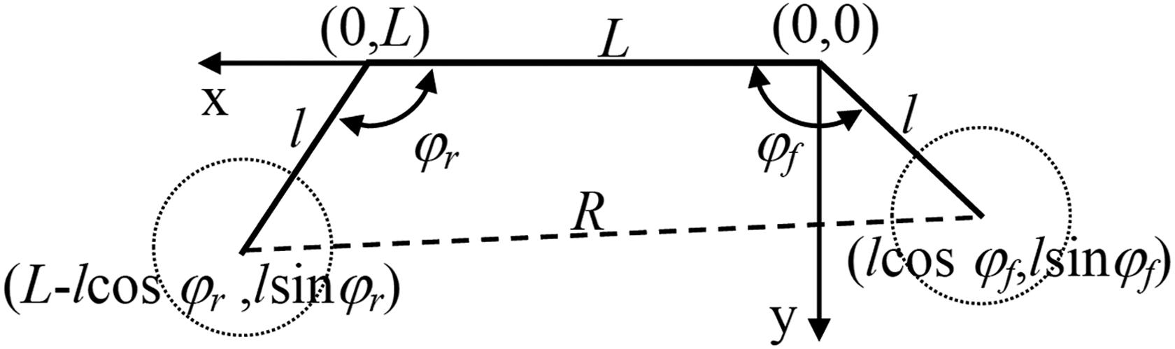
Obtaining the rear and front wheel contact points position vectors, (CP) and (CQ).

Positioning problem

Before addressing the quasi-static approach, a few geometric relationships must be established. The calculation methodology presented in this article requires a solution to positioning problem. For a given ground-track-profile function, f(x), the position of the front wheel, x_f , and the configuration angles, φ_r and φ_f , the problem is reduced to obtaining the position of the rear wheel. To calculate this, the following steps are taken:

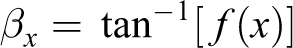
The slope of the ground-track-profile at x is determined as

β_{x} = {tan}^{- 1} [f (x)]

The positions of the centers of the wheels g(s) (see Figure 2) are calculated as

\begin{matrix} s = x - r sin β_{x} \\ f (x) \to g (s) = f (x) + r cos β_{x} \end{matrix}

So that for a given contact of the front wheel x-coordinate, x_f , the position of the center of the front wheel (s_f , g(s_f )) is located.

The wheelbase is solved from Figure 3

R = \sqrt{{(L - l cos φ_{r} - l cos φ_{f})}^{2} + l^{2} {(sin φ_{r} - sin φ_{f})}^{2}}

Finally, the rear wheel center is located on line g at a distance R from the front wheel center. Hence, the wheel center is obtained by the intersection of the circumference of radius R centered on the front wheel and the graph of the function g (see Figure 4).

After the position of the vehicle is located, the rear and front wheel contact point position vectors, taken from C ( $\vec{C P}$ and $\vec{C Q}$ ), are expressed in terms of the configuration angles, φ_r and φ_f , using the following steps:

First, φ₁ and φ₂ (see Figure 5) are expressed in terms of φ_r and φ_f, using the cosine theorem twice (on the triangles Rld and Lld)

\begin{array}{l} R^{2} + l^{2} - 2 R l cos φ_{1} = L^{2} + l^{2} - 2 L l cos φ_{f} \Rightarrow \\ \Rightarrow cos φ_{1} = \frac{R^{2} - L^{2} + 2 L l cos φ_{f}}{2 R l} \end{array}

and by symmetry

cos φ_{2} = \frac{R^{2} - L^{2} + 2 L l cos φ_{r}}{2 R l}

Then, the coordinates of points 1 to 4, in the reference system indicated in Figure 5, are expressed as follows

x_{1} = \frac{l}{2} cos (ψ + φ_{1}); y_{1} = \frac{l}{2} sin (ψ + φ_{1})

x_{2} = l cos (ψ + φ_{1}) + \frac{L}{2} cos (ψ + φ_{1} + φ_{r} - π) - \frac{H}{2} sin (ψ + φ_{1} + φ_{r} - π)

y_{2} = l sin (ψ + φ_{1}) + \frac{L}{2} sin (ψ + φ_{1} + φ_{r} - π) + \frac{H}{2} cos (ψ + φ_{1} + φ_{r} - π)

x_{3} = R cos ψ - \frac{l}{2} cos (φ_{2} - ψ)

y_{3} = R sin ψ + \frac{l}{2} sin (φ_{2} - ψ)

x_{4} = R cos ψ; y_{4} = R sin ψ

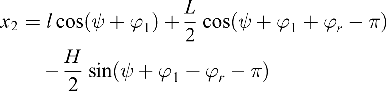
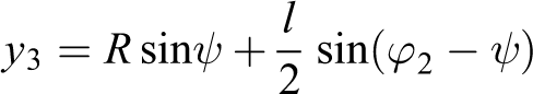
where the wheelbase inclination angle, or pitch angle, ψ is

ψ = {tan}^{- 1} \frac{g (s_{f}) - g (s_{r})}{s_{f} - s_{r}}

Finally, the coordinates for C and those for the ground-wheel contact points P and Q are

C_{x} = \frac{m_{l} x_{1} + m_{r} x_{2} + m_{l} x_{3} + m_{w} x_{4}}{m}

C_{y} = \frac{m_{l} y_{1} + m_{r} y_{2} + m_{l} y_{3} + m_{w} y_{4}}{m}

P_{x} = r sin β_{r}; P_{y} = - r cos β_{r}

Q_{x} = R cos ψ + r sin β_{f}

Q_{y} = R sin ψ - r cos β_{f}

from which the components ${\bar{C P}}_{x}, {\bar{C P}}_{y}, {\bar{C Q}}_{x}$ , and ${\bar{C Q}}_{y}$ are obtained ( ${\bar{C P}}_{x} = P_{x} - C_{x}$ , and so on).

Dynamic problem: Quasi-static

For a quasi-static approach, the UGV is considered to be in equilibrium at every point of its trajectory, so the forces and moments are balanced. Since the torque on both wheels must be the same, when balancing moments about the center of each of the wheels we conclude that the corresponding ground-wheel frictional force is also the same for both (see Figure 6).

Figure 6.

Balancing moments in one wheel.

Note, it has been assumed that the coefficient of the friction force is equal throughout the trajectory, but this could be easily varied. A different coefficient of friction could be defined at each point of the track profile.

Meanwhile, the balance of the whole vehicle system (see Figure 7) requires one moment equation and two force equations. Note, that moments have been calculated with respect to the CoM, C. The unknown variables for the system of equations are F, N_r , and N_f .

Figure 7.

Balance concerning the whole vehicle.

The system can be written in a matrix form

\begin{array}{l} A B = C \Rightarrow B = A^{- 1} C \\ A = (\begin{matrix} (cos β_{r} + cos β_{f}) & - sin β_{r} & - sin β_{f} \\ (sin β_{r} + sin β_{f}) & cos β_{r} & cos β_{f} \\ \begin{matrix} {\bar{C P}}_{x} sin β_{r} - {\bar{C P}}_{y} cos β_{r} + \\ + {\bar{C Q}}_{x} sin β_{f} - {\bar{C Q}}_{y} cos β_{f} \end{matrix} & \begin{matrix} {\bar{C P}}_{x} cos β_{r} + \\ + {\bar{C P}}_{y} sin β_{r} \end{matrix} & \begin{matrix} {\bar{C Q}}_{x} cos β_{f} + \\ + {\bar{C Q}}_{y} sin β_{f} \end{matrix} \end{matrix}) \\ B = (\begin{matrix} F \\ N_{r} \\ N_{f} \end{matrix}) and C = (\begin{matrix} 0 \\ m_{g} \\ 0 \end{matrix}) \end{array}

In summary, for given values of the contact angles, β_r and β_f , the pitch angle, ψ, and the configuration angles, φ_r and φ_f , the previous system of equations provides the value of the friction force, and hence the torque, that must be applied to both wheels in order to maintain the vehicle in equilibrium. The system of equations also provides the values of both ground-wheel normal forces, and so the minimum coefficient of friction required in order to prevent slippage is $μ_{min} \geq Max (\frac{F}{N_{r}}, \frac{F}{N_{f}})$

Iterated algorithm for the model

The previous system of equations has been implemented in a MATLAB code to solve for each point on one discretization of the track, and for each combination of discretized configuration angles. Thus, for a set of discretized positions of the front wheel along the track, the algorithm obtains the torque that needs to be applied to each wheel in order to keep the vehicle in a static position. This is performed for every combination of the discretized values of the configuration angles φ_r and φ_f .

Figure 8 shows how the program executes a three-level discretization (along the track and sweeping for both configuration angles) and obtains (for each combination) the torque and normal forces on the wheels. Having obtained this data, the optimized configuration angles along the track are then achieved by selecting, for every point on the track (position of the front wheel), the values of the angles φ_r and φ_f that meet some criteria. Examples of criteria include the following: “minimum instantaneous torque criterion” that can be applied to minimize the needed energy; “minimum instantaneous torque variation criterion”; “minimum torque whole variation criterion” that can be used for the whole ground-track-profile. Also, the criterion could be to limit the torque variation between points.

Figure 8.

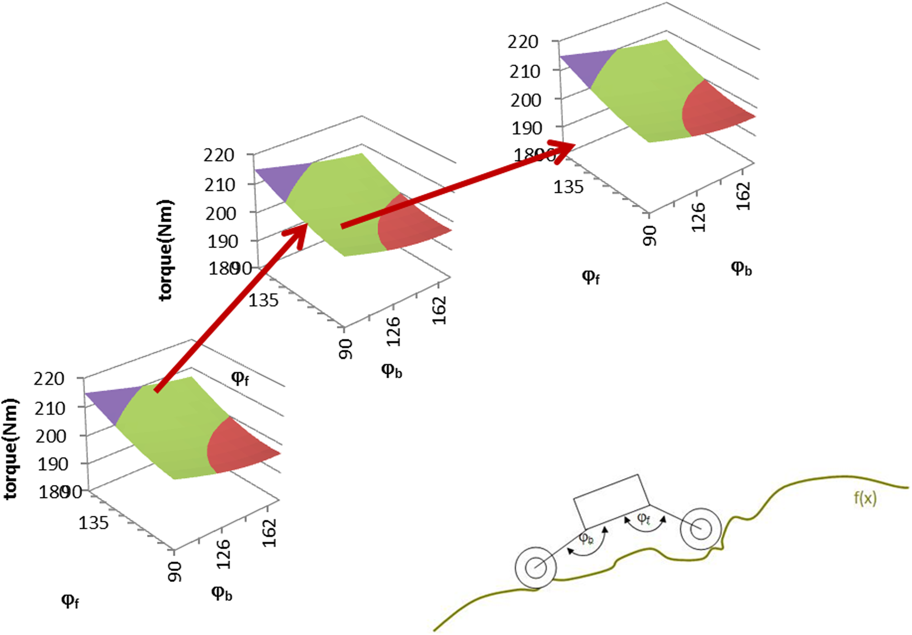
Scheme of the algorithm process.

At the present time, other criteria (like maximum wheel normal force or minimum coefficient of friction), and conditions different from equally distributed torque, are to be used to research on improving UGV passing complicated obstacles.

The inputs of the algorithm are the ground-track-profiles together with the masses and geometrical parameters of the UGV vehicle. The required torque for any configuration angle combination and the combinations of configuration angles that meet the criterion imposed along the ground-track-profile are the outputs of the program.

Simulation results

Some results are shown in order to demonstrate the validity and versatility of the model.

In order to show the robustness of the developed algorithm, some results from different applications are presented. How the dynamic variables change for different profiles, which torque is required in order to go over obstacles, and how the navigation can be optimized comparing multiples trajectories, among others.

The developed algorithm has been used firstly to calculate the torque applied to both wheels and the corresponding normal forces, depending on the slope. In this situation, since the torque does not depend on the configuration angles, the algorithm has been employed to find the configuration that provides the closest normal values. Figure 9 shows the results for the torque and both normal forces. It can be seen that as the slope increases, the more torque is required to maintain the vehicle in quasi-static equilibrium.

Figure 9.

Torque and normal forces for different ramps.

Some examples are shown in Figure 10 for a “soft” bump (square exponential profile, $f (x) = 0.1 e^{- {(x - 4)}^{2}}$ (x in meters)). The torque required is shown. The configuration angles do not vary as the vehicle passes the ground-track-profile.

Figure 10.

Needed torque functions for static configuration angles.

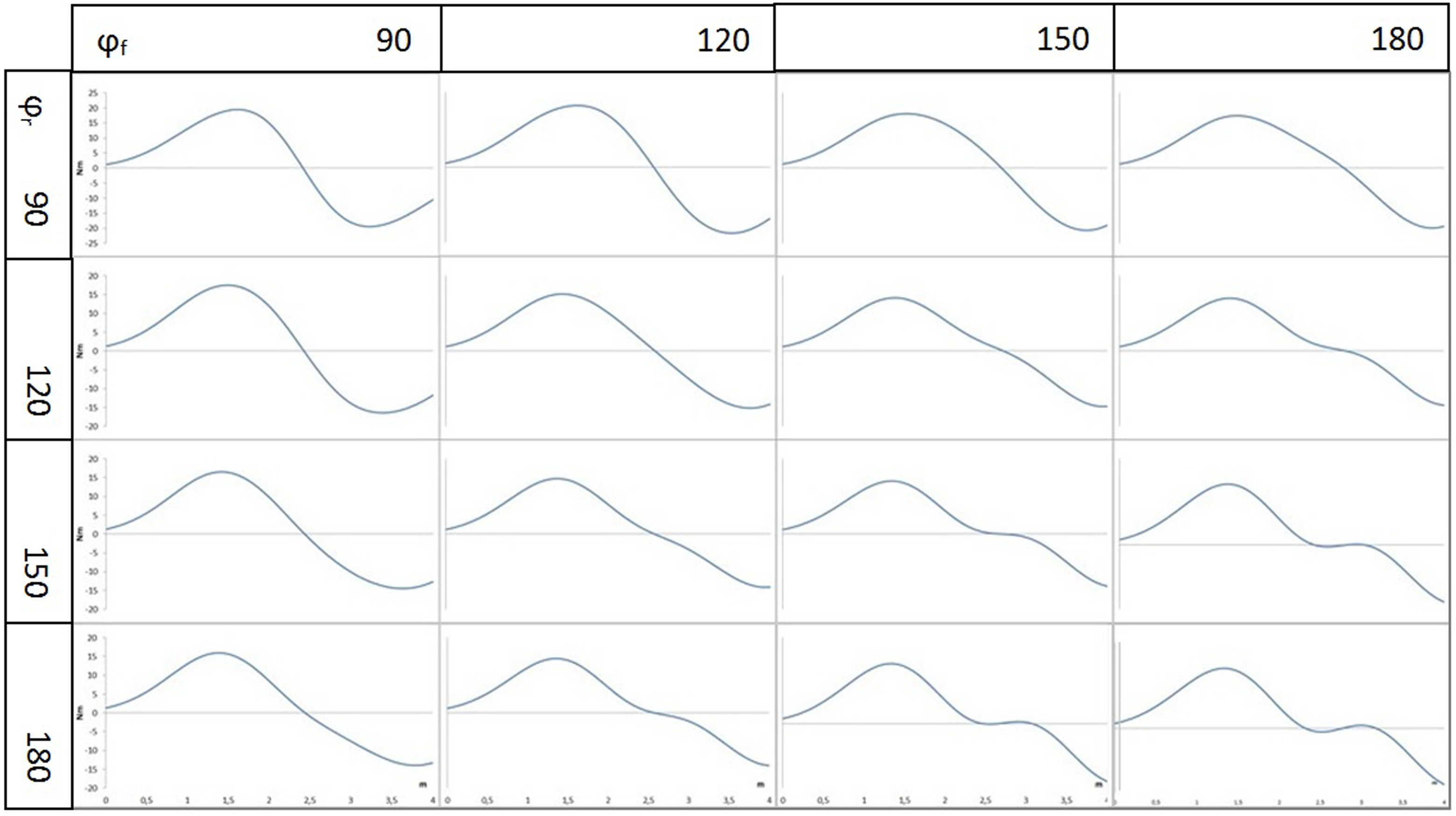
The ground function f(x) = (x + sinx)/2 has been entered to the algorithm. The torque values for the front wheel initial position in function of the configuration angles for one point are shown in Figure 11, and in Figure 12, the minimum torque values are plotted against the front wheel position as it moves along this profile.

Figure 11.

Minimum torque versus φ_f and φ_f for one point.

Figure 12.

Minimum torque while moving.

Figure 13 shows the torque function together with the optimal configuration angle variation needed for the vehicle to pass over the bump with the lowest possible variation of torque applied to the wheels. A sequence of the UGV as it passes through the ground-track-profile is also represented in Figure 14. It can be seen that the torque rises from 0 (where the UGV is at almost in a flat standpoint) to 12.5 Nm, which is the maximum torque needed and corresponds to the highest point reached by the front wheel. The required torque then decreases, as the vehicle descends, reaching negative values, when the vehicle would move downhill (these negative torque values are necessary to prevent the vehicle from rolling over).

Figure 13.

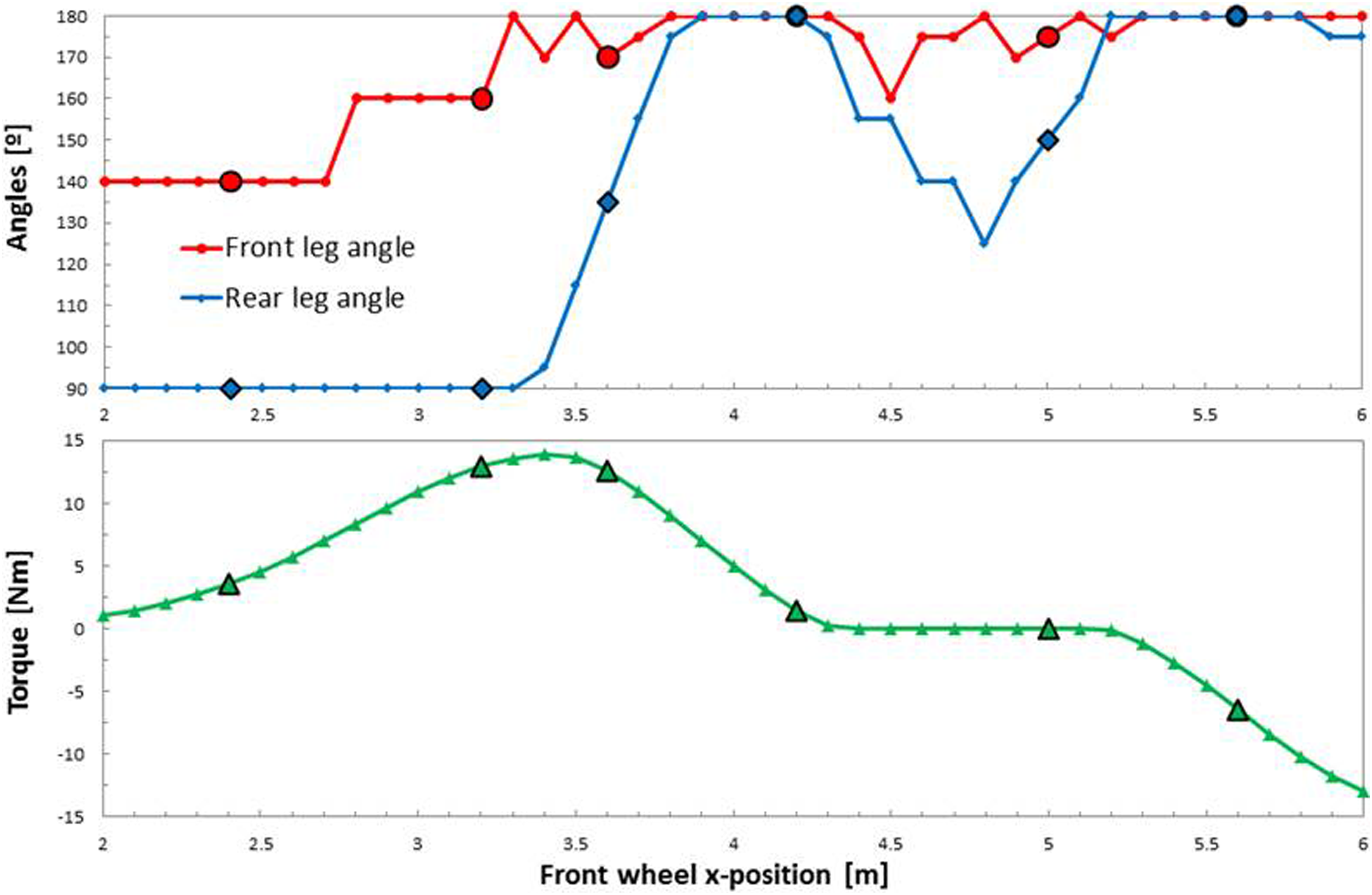
The lowest variation in torque through the bump.

Figure 14.

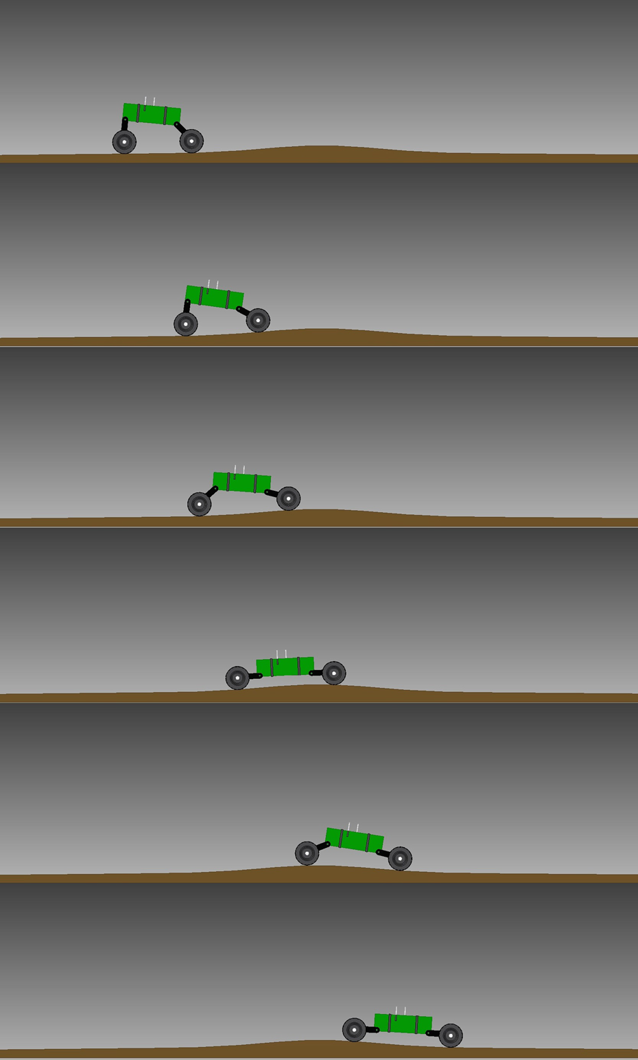
Sequence of the UGV as it passes through the ground-track-profile. UGV: unmanned ground vehicle.

The method can be applied to calculate the torque to get over a step (obstacle with radius less than that of the wheel). In Figure 15, the position of the front wheel is shown and the torque and configuration angles are shown in Figure 15(b) and (c).

Figure 15.

(a) Schema, (b) configuration angles, and (c) needed torque.

This method was used to calculate the configurations that minimize the required torque at each position defined by the angle γ as shown in Figure 15(a).

Optimization results

If the contours of the terrain are known, the previous algorithm can be used for optimizing the navigation. By calculating the energy required to move between the level curves and the best position of the angles φ_r and φ_d , depending on the criterion chosen, the algorithm to calculate the best way is easily programmable (minimum energy, minimum torque variation, maximum ground-wheel normal force, etc.).

Figure 16 shows a contour map and three routes that the UGV could take: direct, intermediate, and smooth. The direct route has a straight trajectory with the biggest slope and the minimum horizontal tour, the smooth route has the longest horizontal tour with the minimum slope, and the intermediate route is in between both of these. The starting point and the end point is the same for the three routes.

Figure 16.

Three different ways obtain with the navigation program.

Figure 17 shows the torque required to be applied on the wheels for these three different routes. It is noted that for the direct route, the highest torque is required, for the least horizontal tour. It is obvious that this route is the fastest if the vehicle is moving with the same velocity for each of the three routes. The direct route requires the highest torque and arrives to the end point via the shortest route. The smooth route requires the minimum amount of torque, but this torque is needed to be applied over a greater time and more tour. Regarding the intermediate route, this does not require such as high a torque as the direct route and it does not take as much time as the smooth route.

Figure 17.

Way obtain with the navigation program. Torque in function of horizontal distance.

The total energy required to ascend the peak is the same, but this approach enables the choice between applying a high torque over less time or a low torque over a greater time, or even the most continuous torque. Although the energy expenditure is the same for all of the routes, with regard to the engine and batteries, the most continuous-as-possible torque is usually preferable, as well as not exceeding a certain maximum torque value. All of this gives us the possibility of optimizing to find the best route to arrive at a point by only knowing the contour map.

Figure 18 shows the front and rear angles obtained with the algorithm for the three routes. For every position on the track, with these angle values, the torque required is shown in Figure 16. This was calculated by optimizing for the minimum torque and the minimum torque variation for every position, while penalizing large variations in configuration angles. This was the chosen criterion for optimization since the high variations in torque are detrimental for the batteries, and rapid changes in the angles are undesirable; the main aim is to find the minimized torque. However, any other criterion of optimization could be chosen.

Figure 18.

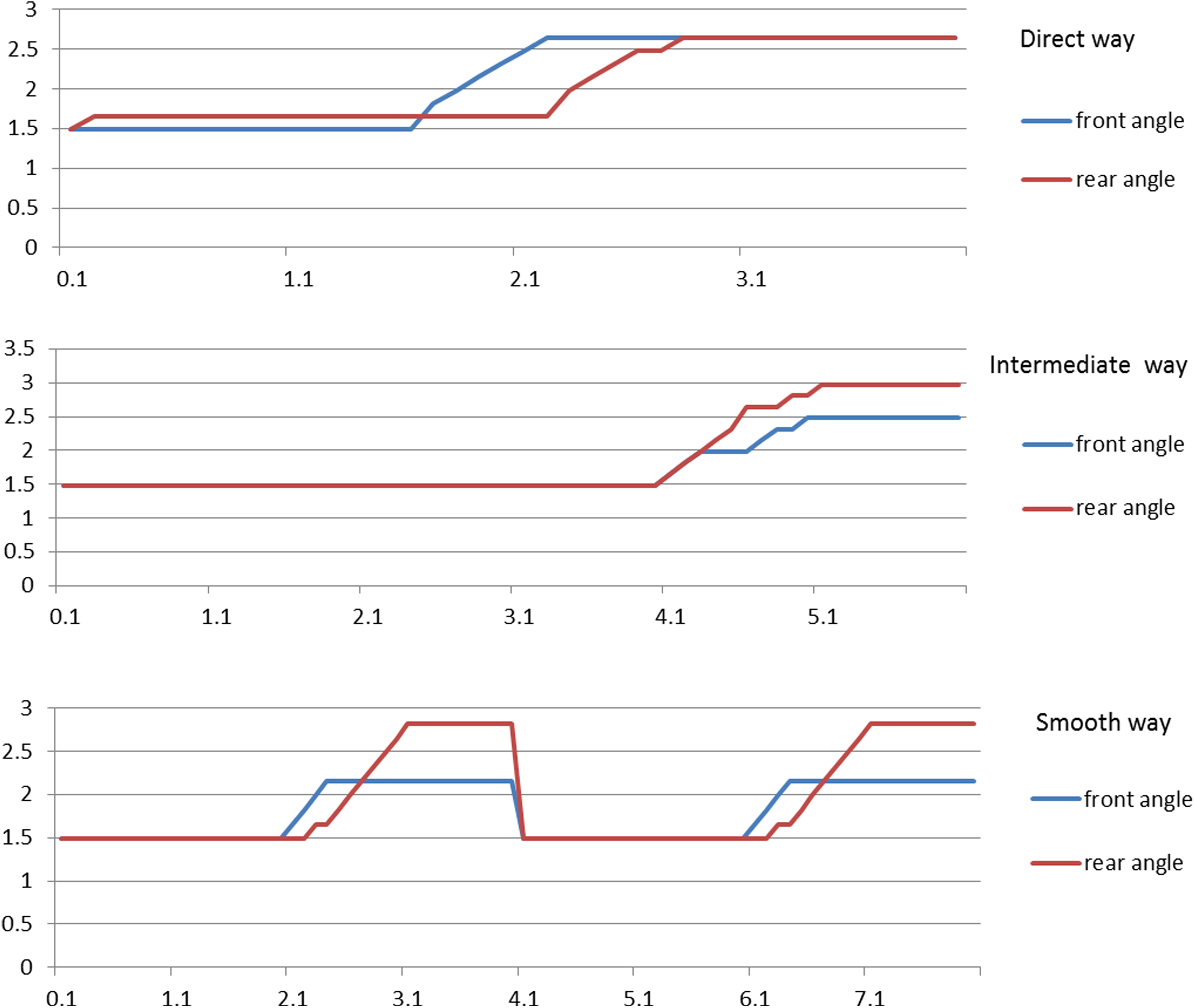
Way obtain with the navigation program. Configurations angles in function of time.

Conclusion

An algorithm for optimizing the torque required and the configuration angles of a UGV as it travels along a certain profile has been presented in this article. It is based on a quasi-static half-vehicle model. This algorithm has been implemented in MATLAB code.

At any point of a given profile (defined by either an analytical function or by a discretized one), the program calculates the torque that must be applied to the front and back wheels for any configuration of the legs with a little computational cost. Furthermore, it determines if the wheels slip at any point on the track and if the vehicle will roll over.

The program is also capable of selecting the optimal path from several options. The criterion for optimization can be chosen depending on the desired goal (minimum energy lost, minimum time, minimum torque needed, etc.). This could be a great tool if the map of the terrain is known in advance, by calculating the best way to go and return, as well as the point of no return. At that point, the UGV will only have sufficient energy to return (although not necessarily by the same route).

This program will be a valuable tool for (i) optimizing some navigation capabilities, for instance: minimizing torque variation on the wheels, maximizing the whole vehicle grip, and improving energy distribution; (ii) designing control strategies for navigating obstacles or complex terrain profiles; and (iii) selecting the best route by optimization, among others.

We believe it can be a very valuable tool to minimize energy expenditure or get the minimum torque to reach a destination. It may be very interesting as future work would compare the theoretical and real results. As well as, get the real and theoretical no-return-points, and the sliding start points.

Another very interesting future work would be to apply this methodology for walking or climbing stairs.

Footnotes

Acknowledgements

The authors wish to thank the Spanish Government for financing provided through the MCYT project “RETOS2015: sistema de monitorización integral de conjuntos mecánicos críticos para la mejora del mantenimiento en el transporte-maqstatus” and also thank the anonymous reviewers for their insightful comments and suggestions on an earlier draft of this article.

Declaration of conflicting interests

The author(s) declared no potential conflicts of interest with respect to the research, authorship, and/or publication of this article.

Funding

The author(s) disclosed receipt of the following financial support for the research, authorship, and/or publication of this article: This work was financially supported by the Spanish Government through the MCYT project “RETOS2015: sistema de monitorización integral de conjuntos mecánicos críticos para la mejora del mantenimiento en el transporte-maqstatus.”

ORCID iD

Eduardo Corral Abad

References

Tallinn University of Technology, Dept. of Mechatronics, “Universal Ground Vehicle,” Research proj. L523, 2005–2008.

Sell

Aryassov

Petritshenko

. Kinematics and dynamics of configurable wheel-leg. In: 8th international conference of DAAAM, Tallinn, Estonia, 19–21 April 2012, pp. 345–350.

Corral

Meneses

Aryassov

. A quasi-static approach to optimize the motion of a UGV depending of the track profile. In: Olegas

Arturas

(eds) 9th international conference MSM, 2013, pp. 41–42. Vilnius, Lithuania: Vilnius Gediminas Technical University Press “Technika”.

Remenyte-Prescott

Andrews

JD,

Chung Bérenguer

PWH

. An efficient phased mission reliability analysis for autonomous vehicles. Reliab Eng Syst Safety 2010; 95: 226–235.

Hasaneini

Macnab

CJB

Bertram

JEA

. The dynamic optimization approach to locomotion dynamics: human-like gaits from a minimally constrained biped model. Adv Robot 2013; 27: 845–859.

Azimi

Yazdi

MRH

. Energy dissipation rate control and parallel equations solving method for planar spined quadruped bouncing robot. J Mech Sci Technol 2017; 31: 875. DOI: 10.1007/s12206-016-0942-7.

Pfeifer

Iida

Bongard

. New robotics: design principles for intelligent systems. Artif Life 2005; 11(1–2): 99–120. DOI: 10.1162/1064546053279017.

Pfeifer

Gomez

. Interacting with the real world: design principles for intelligent systems. Artif Life Robot 2005; 9: 1. DOI: 10.1007/s10015-004-0343-3.

Pfeifer

Bongard

. How the body shapes the way we think: a new view of intelligence. Cambridge: MIT Press.

10.

Posa

Kuindersma

Tedrake

. Optimization and stabilization of trajectories for constrained dynamical systems. In: 2016 IEEE international conference on robotics and automation (ICRA), Stockholm, 16–21 May 2016, pp. 1366–1373. DOI: 10.1109/ICRA.2016.7487270.

11.

Wardana

Takaki

Aoyama

. Development of a control system for a stair-climbing inverted pendulum robot. In: 2016 international conference on instrumentation, control and automation (ICA), Bandung, 9–31 August 2016, pp. 1–5. DOI: 10.1109/ICA.2016.7811465.

12.

Meneses

Castejón

Corral

. Kinematics and dynamics of the quasi-passive biped “PASIBOT.” Strojniški Vestnik J Mech Eng 2011; 57(12): 879–887.

13.

Corral

Meneses

Castejón

. Forward and inverse dynamics of the biped PASIBOT. Int J Adv Robot Syst 2014; 11: 109. DOI: 10.5772/58537.

14.

Fujimoto

Minimum energy trajectory planning for biped robots. In: Armando Carlos de Pina

Filho

(ed) Humanoid robots: new developments. InTech, http://www.intechopen.com/books/humanoid_robots_new_developments/minimum_energy_trajectory_planning_for_biped_robots (2007, accessed 05 June 2013).

15.

Jang

Bae

Park

. Research of velocity control on the slope road for unmanned ground vehicle. In: International conference on control, automation and systems 2010, 27–30 October 2010, KINTEX, Gyeonggi-do, Korea.

16.

Hiiemaa

Tamre

. Assisting control algorithms for simplified operation of remotely controlled unmanned ground vehicle. In: 7th international conference MSM, Kaunas University of Technology, 7–9 July 2011, Kaunas, Lithuania.

17.

Di Giandomenico

Itria

Masci

. Automated synthesis of dependable mediators for heterogeneous interoperable systems. Reliab Eng Syst Safety 2014; 132: 220–232. DOI: 10.1016/j.ress.2014.08.001.

18.

Kappaganthu

Nataraj

. Optimal biped design using a moving torso: theory and experiments. In: Armando Carlos Pina

Filho

(ed) Biped robots. InTech, http://www.intechopen.com/books/bipedrobots/optimal-biped-design-using-a-movingtorsotheory-and-experiments (2011, accessed 05 June 2013).

19.

Proactivity and Behavioural Models of Mechatronic and Production Systems, TTU, Research project SF0140113Bs08, 2008–2013.

20.

Bouvard

Artus

Bérenguer

. Condition-based dynamic maintenance operations planning & grouping. Appl Commerc Heavy Veh Reliab Eng Syst Safety 2011; 96: 601–610.

21.

Barros

. Maintenance grouping strategy for multi-component systems with dynamic contexts. Reliab Eng Syst Safety 2014; 132: 233–249. DOI: 10.1016/j.ress.2014.08.002.

22.

Newton

1687, Mathematical principles of nature philosophy and his systems of the world. In: Cohen

Whitman

. Berkeley, California: University of California Press, 1999.

23.

Corral

Aryassov

Meneses

. A quasi-static approach to optimize the motion of an UGV depending on the track profile. In: Solid State Phenomena, vol. 220–221. Switzerland: Trans Tech Publications, 2015, pp. 774–780. DOI: 10.4028/www.scientific.net/SSP.220-221.774.

24.

Dunlap

Caldwell

Collins

Jr . Motion planning for mobile robots via sampling-based model predictive optimization. In: Topalov

(ed) Recent advances in mobile robotics. ISBN: 978-953-307-909-7, InTech, http://www.intechopen.com/books/recent-advances-in-mobile-robotics/motion-planning-for-mobile-robots-viasampling-based-model-predictive-optimization (accessed 01 October 2017).

25.

Hosseini

Barker

Ramirez-Marquez

. A review of definitions and measures of system resilience. Reliab Eng Syst Safety 2016; 145: 47–61. DOI: 10.1016/j.ress.2015.08.006.

26.

Zhang

Chen

. A practical approach for solving multi-objective reliability redundancy allocation problems using extended bare-bones particle swarm optimization. Reliab Eng Syst Safety 2014; 127: 65–76. DOI: 10.1016/j.ress.2014.03.006.

27.

Galbrun

Pelechrinis

Terzi

. Urban navigation beyond shortest route: the case of safe paths. Inform Syst 2016; 57: 160–171. DOI: 10.1016/j.is.2015.10.005.

28.

López-Santana

Akhavan-Tabatabaei

Dieulle

. On the combined maintenance and routing optimization problem. Reliab Eng Syst Safety 2016; 145: 199–214.

Methodology for the navigation optimization of a terrain-adaptive unmanned ground vehicle

Abstract

Keywords

Introduction

Nomenclature

Positioning problem

Dynamic problem: Quasi-static

Iterated algorithm for the model

Simulation results

Optimization results

Conclusion

Footnotes

Acknowledgements

Declaration of conflicting interests

Funding

ORCID iD

References